Electronic Thesis and Dissertation Repository
8-21-2019 2:00 PM
Towards Using Model Averaging To Construct Confidence
Towards Using Model Averaging To Construct Confidence
Intervals In Logistic Regression Models
Intervals In Logistic Regression Models
Artem Uvarov
The University of Western Ontario
Supervisor Zou, Guangyong
The University of Western Ontario
Graduate Program in Epidemiology and Biostatistics
A thesis submitted in partial fulfillment of the requirements for the degree in Doctor of Philosophy
© Artem Uvarov 2019
Follow this and additional works at: https://ir.lib.uwo.ca/etd
Part of the Statistical Methodology Commons
Recommended Citation Recommended Citation
Uvarov, Artem, "Towards Using Model Averaging To Construct Confidence Intervals In Logistic Regression Models" (2019). Electronic Thesis and Dissertation Repository. 6388.
https://ir.lib.uwo.ca/etd/6388
This Dissertation/Thesis is brought to you for free and open access by Scholarship@Western. It has been accepted for inclusion in Electronic Thesis and Dissertation Repository by an authorized administrator of
Regression analyses in epidemiological and medical research typically begin with a model
selection process, followed by inference assuming the selected model has generated the data
at hand. It is well-known that this two-step procedure can yield biased estimates and invalid
confidence intervals for model coefficients due to the uncertainty associated with the model
selection. To account for this uncertainty, multiple models may be selected as a basis for
inference. This method, commonly referred to as model-averaging, is increasingly becoming
a viable approach in practice.
Previous research has demonstrated the advantage of model-averaging in reducing bias of
parameter estimates. However, there is lack of methods for constructing confidence intervals
around parameter estimates using model-averaging. In the context of multiple logistic
regres-sion models, we propose and evaluate new confidence interval estimation approaches for
re-gression coefficients. Specifically, we study the properties of confidence intervals constructed
by averaging tail errors arising from confidence limits obtained from all models included in
model-averaging for parameter estimation. We propose model-averaging confidence intervals
based on the score test. For selection of models to be averaged, we propose the bootstrap
inclusion fractions method.
We evaluate the performance of our proposed methods using simulation studies, in a
com-parison with model-averaging interval procedures based on likelihood ratio and Wald tests,
tra-ditional stepwise procedures, the bootstrap approach, penalized regression, and the Bayesian
model-averaging approach.
Methods with good performance have been implemented in the ‘mataci’ R package, and
illustrated using data from a low birth weight study.
KEYWORDS: Model-averaging; Logistic regression; Confidence interval; Score function.
Data analysis in medical research often involves regression analysis that examines the
associations between outcome and independent variables. Analysis consists of selection of
these variables and estimation of their effects. A point estimate usually varies from sample
to sample, meaning that the estimated effect has some distribution. The 95% confidence
interval, a range around a point estimate within which the true effect is likely to fall, is used
to quantify the uncertainty associated with the estimates. Tail errors on both sides of a valid
confidence interval should be similar and close to the specified limit.
Unfortunately, using the same data to construct confidence intervals usually leads to
biased results, especially in small samples. The coverage of confidence intervals obtained
by such “double use” of the data is often below the specified limit. To address this problem,
it was proposed to use several regression models, which results are averaged. The selection
of candidate models is important for the averaging process. If done correctly it allows one
to accelerate the computations and also to improve precision of results, while a insufficient
set of models can negatively affect the final conclusions.
Model-averaging makes it possible to obtain more accurate point estimates, but many
methods for constructing confidence intervals for such averaged estimates suffer from
in-accuracy, especially if samples sizes are not large. Such intervals are often too short, and
the confidence level is much lower than the specified level.
In this work, we proposed an approach for selecting candidate models that reduces the
number of required models, but saves the information that can be obtained from the data.
We also proposed a method that constructs valid and accurate confidence intervals for
re-gression coefficients even for small samples. We used a method that suggests averaging the
tail errors over selected candidate models. The developed methods are more accurate, but
are less traditional variants of the model-averaged tail error method. We focused on
build-ing confidence intervals for logistic regression models that evaluate the effect of variables
on a binary dependent variable. To demonstrate the superiority of the proposed methods,
This research would have been impossible without the aid and support of many
amaz-ing people. There are no proper words to convey my deep gratitude and respect to my
Ph.D. supervisor, Dr. GuangYong Zou for his patient guidance, insightful comments and
invaluable experience I gained. I cannot imagine a better supervisor to learn from. In the
most difficult time, he found words that supported and encouraged me.
I would like to thank Dr. Yun-Hee Choi, for a tremendous help as a supervisory
com-mittee member in editing and shaping this work. Her optimism and helpful suggestions
gave me confidence that I was on the right track. I would also like to acknowledge Dr.
John Koval, Dr. Wenqing He and Dr. Ricardas Zitikis for their helpful suggestions and
constructive comments that allowed me to generalize and improve this study.
I am indebted to my beloved family and closest friends for their inexhaustible moral
support and encouragement over these years. Despite the long distance between us, they
always felt when I needed their wise counsel and sympathetic ears.
This work has been partly financially supported by the Western Graduate Research
Scholarship. I would like to thank the partial financial support from Ontario
Neurodegen-erative Disease Research Initiative (ONDRI). I would also like to thank St. Joseph Hospital,
in particular, Dr. Jeff Mahon, Dr. Tamara Spaic and Dr. Selina Liu from the
endocrinol-ogy department for partial financial support and priceless experience I gained working with
them.
Abstract ii
Summary for Lay Audience iii
Acknowledgments iv
List of Tables viii
List of Figures xv
Chapter 1 INTRODUCTION 1
Chapter 2 OVERVIEW OF VARIABLE SELECTION AND CONFIDENCE
INTERVAL CONSTRUCTION METHODS 10
2.1 Automated model selection . . . 10
2.1.1 Stepwise selection . . . 11
2.1.1.1 Inclusion and exclusion criteria . . . 11
2.1.1.2 The number of events per variable . . . 13
2.1.2 Concerns on stepwise selection . . . 15
2.1.3 Bootstrapped stepwise selection and inference . . . 16
2.1.4 Common approaches to confidence interval estimation . . . 17
2.2 Penalized regression models . . . 19
2.3 Uncertainty and post-selection inference . . . 22
2.3.1 Uncertainty in model selection . . . 22
2.3.2 Post-selection inference . . . 23
2.3.3 Bayesian model-averaging . . . 25
2.3.4 Frequentists model-averaging . . . 27
2.3.5 Confidence intervals following model-averaging . . . 29
3.2 Parsimony principle and accuracy . . . 36
3.3 Candidate models selection based on inclusion fraction . . . 38
Chapter 4 IMPROVING THE WALD MODEL-AVERAGING CONFIDENCE INTERVALS 40 4.1 Introduction . . . 40
4.2 Model-averaged intervals based on score test . . . 41
4.3 Confidence intervals based on Wald standard errors . . . 43
4.4 Wald MATA corrected by the profile-likelihood and score standard errors . 44 4.5 Confidence intervals based on Bayesian model-averaging . . . 45
Chapter 5 EVALUATION OF CONFIDENCE INTERVAL PROCEDURES 46 5.1 Introduction . . . 46
5.2 Confidence interval construction methods . . . 46
5.3 Comparison procedure . . . 48
5.4 Choice of parameters in simulation . . . 51
5.5 Data generation . . . 55
5.6 Software and packages . . . 56
5.7 Results . . . 57
5.7.1 Sample size . . . 57
5.7.2 Number of predictors . . . 69
5.7.3 Correlation . . . 81
5.7.4 Probability of outcome . . . 93
5.8 Discussion . . . 104
5.9 Conclusion . . . 109
Chapter 6 R-PACKAGE 110 6.1 Introduction . . . 110
6.2 The MATACI package . . . 111
6.2.1 The MATACI function . . . 111
6.3 Limitations and further updates . . . 116
Chapter 7 ILLUSTRATIVE EXAMPLE 118 7.1 Introduction . . . 118
7.2 Methods . . . 120
7.3 Results . . . 120
Chapter 8 SUMMARY 127 8.1 Introduction . . . 127
8.2 Main findings and recommendations . . . 128
8.3 Study assumptions and limitations . . . 129
8.4 Directions for future research . . . 130
Bibliography 134 Appendix A 144 A.1 Data generation . . . 144
A.2 Function MATACI . . . 146
A.3 Support functions . . . 150
Curriculum Vitae 162
5.1 Parameter combinations used for simulation study. N sample size, p -number of predictors,ρ - correlation among predictors, Pr - event probability. 54
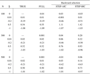
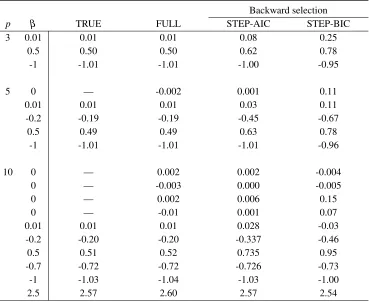
5.2.A Mean of point estimates obtained from the true model, the full model, step-wise AIC and stepstep-wise BIC backward selection methods for different sam-ple sizes, whereρ =0.5 and outcome probability is 50%. The true and the
full model results are based on 1,000 simulations, the results of backward selection methods are based on 10,000 simulations. . . 58
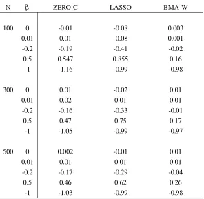
5.2.B Mean of point estimates obtained from the zero-corrected backward se-lection, LASSO, and Wald based Bayesian model-averaging methods for different sample sizes, where ρ =0.5 and outcome probability is 50%.
The LASSO results are based on 10,000 simulations, the results of zero-corrected backward selection and Wald based Bayesian model-averaging are based on 5,000 simulations. . . 59
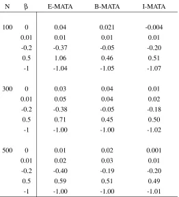
5.2.C Mean of point estimates of the backward stepwise selection (E-MATA), Oc-cam’s window (B-MATA) and inclusion fraction (I-MATA) based model-averaging tail area methods for different sample sizes, whereρ =0.5 and
outcome probability is 50%. The backward stepwise selection and Occam’s window means are based on 5,000 simulations, the results obtained from inclusion fraction are based on 1,000 simulations. . . 60
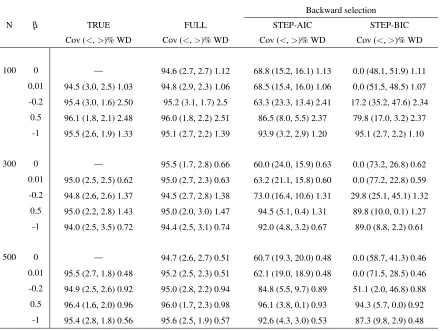
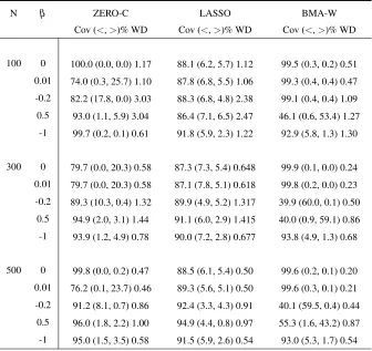
5.2.D Empirical coverage (Cov), tail errors (<,>)% and averaged width (WD) of 95% CIs constructed by the true model, the full model, stepwise AIC and stepwise BIC backward selection methods for different sample sizes, where
ρ=0.5 and outcome probability is 50%. The true and the full model results
are based on 1,000 simulations, the results of backward selection methods are based on 10,000 simulations. . . 61
5.2.E Empirical coverage (Cov), tail errors (<, >)% and averaged width (WD) of 95% CIs constructed by the zero-corrected backward selection, LASSO and Wald based Bayesian model-averaging methods for different sample sizes, whereρ =0.5 and outcome probability is 50%. The LASSO results
are based on 10,000 simulations, the results of zero-corrected and Bayesian approaches are based on 5,000 simulations. . . 62
proach for 95% nominal level based on 5,000 simulations, where ρ =0.5
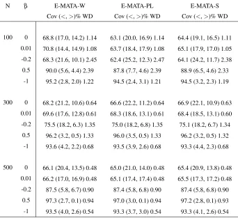
and outcome probability is 50%; Wald based E-MATA-W, profile-likelihood based E-MATA-PL, and score function based E-MATA-S. . . 63
5.2.G Empirical coverage (Cov), tail errors (<, >)% and averaged width (WD) of five model-averaging CI construction methods for different sample sizes using set of candidate models obtained from Occam’s window approach for 95% nominal level based on 5,000 simulations, whereρ=0.5 and outcome
probability is 50%; Wald based MATA-W, profile-likelihood based B-MATA-PL, score function based B-MATA-S, Wald based method corrected by the profile-likelihood B-MATA-Wpl, and Wald based method corrected by the score function B-MATA-Ws. . . 64
5.2.H Empirical coverage (Cov), tail errors (<,>)% and averaged width (WD) of five model-averaging CI construction methods for different sample sizes us-ing set of candidate models obtained from 50% inclusion fraction approach for 95% nominal level based on 1,000 simulations, whereρ =0.5 and
out-come probability is 50%; Wald based I-MATA-W, profile-likelihood based I-MATA-PL, score function based I-MATA-S, Wald based method corrected by the profile-likelihood I-MATA-Wpl, and Wald based method corrected by the score function I-MATA-Ws. . . 65
5.3.A Mean of point estimates obtained from the true model, the full model, step-wise AIC and stepstep-wise BIC backward selection methods for different num-ber of covariates, where N=500,ρ =0.5 and outcome probability is 30%.
The true and the full model results are based on 1,000 simulations, the re-sults of backward selection methods are based on 10,000 simulations. . . 70
5.3.B Mean of point estimates obtained from the zero-corrected backward selec-tion, LASSO and Wald based Bayesian model-averaging methods for dif-ferent number of covariates, where N=500,ρ=0.5 and outcome
probabil-ity is 30%. The LASSO results are based on 10,000 simulations, the re-sults of zero-corrected backward selection and Wald based Bayesian model-averaging are based on 5,000 simulations. . . 71
5.3.C Mean of point estimates of the backward stepwise selection (E-MATA), Oc-cam’s window (B-MATA) and inclusion fraction (I-MATA) based model-averaging tail area methods for different number of covariates, where N=500,
ρ =0.5 and outcome probability is 30%. The backward stepwise selection
and Occam’s window means are based on 5,000 simulations, the results ob-tained from inclusion fraction are based on 1,000 simulations. . . 72
ates, where N=500,ρ =0.5 and outcome probability is 30%. The true and
the full model results are based on 1,000 simulations, the results of back-ward selection methods are based on 10,000 simulations. . . 74
5.3.E Empirical coverage (Cov), tail errors (<, >)% and averaged width (WD) of 95% CIs constructed by the zero-corrected backward selection, LASSO and Wald based Bayesian model-averaging methods for different number of covariates, where N=500,ρ =0.5 and outcome probability is 30%. The
LASSO results are based on 10,000 simulations, the results of zero-corrected and Bayesian approaches are based on 5,000 simulations. . . 75
5.3.F Empirical coverage (Cov), tail errors (<, >)% and averaged width (WD) of three model-averaging CI construction methods for different number of covariates using set of candidate models obtained from backward AIC se-lection approach for 95% nominal level based on 5,000 simulations, where N=500,ρ =0.5 and outcome probability is 30%; Wald based E-MATA-W,
profile-likelihood based E-MATA-PL, and score function based E-MATA-S. 76
5.3.G Empirical coverage (Cov), tail errors (<, >)% and averaged width (WD) of five model-averaging CI construction methods for different number of covariates using set of candidate models obtained from Occam’s window approach for 95% nominal level based on 5,000 simulations, where N=500,
ρ =0.5 and outcome probability is 30%; Wald based B-MATA-W,
profile-likelihood based B-MATA-PL, score function based B-MATA-S, Wald based method corrected by the profile-likelihood B-MATA-Wpl, and Wald based method corrected by the score function B-MATA-Ws. . . 77
5.3.H Empirical coverage (Cov), tail errors (<,>)% and averaged width (WD) of five model-averaging CI construction methods for different number of co-variates using set of candidate models obtained from 50% inclusion fraction approach for 95% nominal level based on 1,000 simulations, where N=500,
ρ =0.5 and outcome probability is 30%; Wald based I-MATA-W,
profile-likelihood based I-MATA-PL, score function based I-MATA-S, Wald based method corrected by the profile-likelihood I-MATA-Wpl, and Wald based method corrected by the score function I-MATA-Ws. . . 78
5.4.B Mean of point estimates obtained from the zero-corrected backward selec-tion, LASSO and Wald based Bayesian model-averaging methods for dif-ferent correlation levels between five covariates, where N=300 and outcome probability is 30%. The LASSO results are based on 10,000 simulations, the results of zero-corrected backward selection and Wald based Bayesian model-averaging are based on 5,000 simulations. . . 82
is 30%. The true and the full model results are based on 1,000 simulations, the results of backward selection methods are based on 10,000 simulations. . 83
5.4.C Mean of point estimates of the backward stepwise selection (E-MATA), Oc-cam’s window (B-MATA) and inclusion fraction (I-MATA) based model-averaging tail area methods for different correlation levels between five co-variates, where N=300 and outcome probability is 30%. The backward step-wise selection and Occam’s window means are based on 5,000 simulations, the results obtained from inclusion fraction are based on 1,000 simulations. . 84
5.4.D Empirical coverage (Cov), tail errors (<,>)% and averaged width (WD) of 95% CIs constructed by the true model, the full model, stepwise AIC and stepwise BIC backward selection methods for different correlation levels between five covariates, where N=300 and outcome probability is 30%. The true and the full model results are based on 1,000 simulations, the results of backward selection methods are based on 10,000 simulations. . . 85
5.4.E Empirical coverage (Cov), tail errors (<, >)% and averaged width (WD) of 95% CIs constructed by the zero-corrected backward selection, LASSO and Wald based Bayesian model-averaging methods for different correlation levels between five covariates, where N=300 and outcome probability is 30%. The LASSO results are based on 10,000 simulations, the results of zero-corrected and Bayesian approaches are based on 5,000 simulations. . . 86
5.4.F Empirical coverage (Cov), tail errors (<, >)% and averaged width (WD) of three model-averaging CI construction methods for different correlation levels between five covariates using set of candidate models obtained from backward AIC selection approach for 95% nominal level based on 5,000 simulations, where N=300 and outcome probability is 30%; Wald based E-MATA-W, profile-likelihood based E-MATA-PL, and score function based E-MATA-S. . . 88
5.4.G Empirical coverage (Cov), tail errors (<, >)% and averaged width (WD) of five model-averaging CI construction methods for different correlation levels between five covariates using set of candidate models obtained from Occam’s window approach for 95% nominal level based on 5,000 simula-tions, where N=300 and outcome probability is 30%; Wald based B-MATA-W, profile-likelihood based B-MATA-PL, score function based B-MATA-S, Wald based method corrected by the profile-likelihood B-MATA-Wpl, and Wald based method corrected by the score function B-MATA-Ws. . . 89
inclusion fraction approach for 95% nominal level based on 1,000 simula-tions, where N=300 and outcome probability is 30%; Wald based I-MATA-W, profile-likelihood based I-MATA-PL, score function based I-MATA-S, Wald based method corrected by the profile-likelihood I-MATA-Wpl, and Wald based method corrected by the score function I-MATA-Ws. . . 90
5.5.A Mean of point estimates obtained from the true model, the full model, step-wise AIC and stepstep-wise BIC backward selection methods for different out-come probabilities, where N=500 andρ =0.3. The true and the full model
results are based on 1,000 simulations, the results of backward selection methods are based on 10,000 simulations. . . 94
5.5.B Mean of point estimates obtained from the zero-corrected backward selec-tion, LASSO and Wald based Bayesian model-averaging methods for differ-ent outcome probabilities, where N=500 andρ =0.3. The LASSO results
are based on 10,000 simulations, the results of zero-corrected backward se-lection and Wald based Bayesian model-averaging are based on 5,000 sim-ulations. . . 95
5.5.C Mean of point estimates of the backward stepwise selection (E-MATA), Oc-cam’s window (B-MATA) and inclusion fraction (I-MATA) based model-averaging tail area methods for different outcome probabilities, where N=500 andρ=0.3. The backward stepwise selection and Occam’s window means
are based on 5,000 simulations, the results obtained from inclusion fraction are based on 1,000 simulations. . . 96
5.5.D Empirical coverage (Cov), tail errors (<,>)% and averaged width (WD) of 95% CIs constructed by the true model, the full model, stepwise AIC and stepwise BIC backward selection methods for different outcome probabil-ities, where N=500 and ρ =0.3. The true and the full model results are
based on 1,000 simulations, the results of backward selection methods are based on 10,000 simulations. . . 97
5.5.E Empirical coverage (Cov), tail errors (<, >)% and averaged width (WD) of 95% CIs constructed by the zero-corrected backward selection, LASSO and Wald based Bayesian model-averaging methods for different outcome probabilities, where N=500 andρ =0.3. The LASSO results are based on
10,000 simulations, the results of zero-corrected and Bayesian approaches are based on 5,000 simulations. . . 98
tion approach for 95% nominal level based on 5,000 simulations, where N=500 and ρ =0.3; Wald based MATA-W, profile-likelihood based
E-MATA-PL, and score function based E-MATA-S. . . 99
5.5.G Empirical coverage (Cov), tail errors (<,>)% and averaged width (WD) of five model-averaging CI construction methods for different outcome prob-abilities using set of candidate models obtained from Occam’s window ap-proach for 95% nominal level based on 5,000 simulations, where N=500 and ρ =0.3; Wald based W, profile-likelihood based
B-MATA-PL, score function based B-MATA-S, Wald based method corrected by the profile-likelihood B-MATA-Wpl, and Wald based method corrected by the score function B-MATA-Ws. . . 100
5.5.H Empirical coverage (Cov), tail errors (<,>)% and averaged width (WD) of five model-averaging CI construction methods for different outcome prob-abilities using set of candidate models obtained from 50% inclusion frac-tion approach for 95% nominal level based on 1,000 simulafrac-tions, where N=500 and ρ =0.3; Wald based MATA-W, profile-likelihood based
I-MATA-PL, score function based I-MATA-S, Wald based method corrected by the profile-likelihood I-MATA-Wpl, and Wald based method corrected by the score function I-MATA-Ws. . . 101
6.1 Description of the ‘mataci’ function arguments. . . 112
7.1 Point estimates of low birth weight risk factors obtained by the full model (FULL), stepwise AIC backward selection (STEP-AIC), stepwise BIC back-ward selection (STEP-BIC), zero-corrected backback-ward selection (ZERO-C), LASSO and Wald type BMA (BMA-W). . . 121
7.2 Point estimates of low birth weight risk factors obtained by the frequentist model-averaging procedures based on the candidate models from backward selection (E-MATA), Occam’s window (B-MATA) methods and 50% inclu-sion fraction (I-MATA). . . 122
7.3 Confidence interval [L,U] and width WD for low birth weight risk factors obtained by the full model (FULL) and five I-MATA based meth-ods; Wald based I-MATA-W, profile-likelihood based I-MATA-PL, score function based I-MATA-S, Wald based method corrected by the profile-likelihood I-MATA-Wpl, and Wald based method corrected by the score function I-MATA-Ws. . . 123
LASSO and Wald type Bayesian model-averaging (BMA-W). . . 124
7.5 Confidence interval[L,U] and widthWD for low birth weight risk fac-tors obtained by five model-averaging CI construction methods using set of candidate models obtained from backward AIC selection approach; Wald based E-MATA-W, profile-likelihood based E-MATA-PL, and score func-tion based E-MATA-S. . . 125
7.6 Confidence interval[L,U] and widthWD for low birth weight risk fac-tors obtained by three model-averaging CI construction methods using set of candidate models obtained from Occam’s window approach; Wald based MATA-W, profile-likelihood based MATA-PL, score function based S, Wald based method corrected by the profile-likelihood B-MATA-Wpl, and Wald based method corrected by the score function B-MATA-Ws. . 126
5.1 Comparison of averaged widths of the full model- , I-MATA-Wpl - , I-MATA-PL - , I-MATA-W - , I-MATA-Ws - , I-MATA-S - for sample sizes: (a) - N=100, (b) - N=300, and (c) - N=500. . . 68
5.2 Comparison of averaged widths of the full model- , I-MATA-Wpl - , I-MATA-PL - , I-MATA-W - , I-MATA-Ws - , I-MATA-S - for number of variables: (a) - p=3, (b) - p=5, and (c) - p=10. . . 80
5.3 Comparison of averaged widths of the full model- , I-MATA-Wpl - , I-MATA-PL - , I-MATA-W - , I-MATA-Ws - , I-MATA-S - for correlations: (a) -ρ=0.3, (b) -ρ=0, and (c) -ρ=0.5. . . 92
5.4 Comparison of averaged widths of the full model- , I-MATA-Wpl - , I-MATA-PL - , I-MATA-W - , I-MATA-Ws - , I-MATA-S - for outcome probabilities: (a) - Pr=0.1, (b) - Pr=0.3, and (c) - Pr=0.5. . . 103
6.1 Example of inclusion fraction based MATA-S results provided by the mataci function for low birth weight data. . . 115
7.1 Visualization and summary statistics of all risk factors for children’s low birth weight. . . 119
Chapter 1
INTRODUCTION
Routine data analysis in epidemiologic or health sciences research is typically
con-ducted by first selecting a model, followed by obtaining point estimates and standard errors
as well as p-values. The same data set is used for both model selection and statistical
in-ference. When separate data sets are use separately for each purpose, results are usually
valid. However, the use of the same data set repeatedly can lead to incorrect estimation of
standard errors, biased p-values and invalid confidence intervals (Berk et al., 2010;
Freed-man et al., 1988). This is because traditional inference procedures are usually developed
by assuming a given correct model. Yet the model selection process usually involves
mul-tiple comparisons of the models. Such data snooping can lead to a misspecified model and
increased Type I error.
This problem has long been documented in the literature (e.g. P¨otscher, 1991 and
Kabaila, 2005). Leeb and P¨otscher (2005) and Leeb (2006) pointed out that the
distri-bution of post-selected variables cannot be estimated because the estimation error is not
uniformly small even if the sample size goes to infinity. Nevertheless, a review by Walter
and Tiemeier (2009) showed that 20% of the articles published in the four leading
epidemi-ological journals in 2008 used either forward or backward stepwise selection methods. A
recent review done by Fern´andez-Ni˜no et al. (2018) found that stepwise selection based
methods were used in 50% of the published articles between 2000 and 2017. These
principled analytical procedures.
Common model selection procedures usually result in a single final model, which is
then assumed to be the true model upon which the subsequent statistical inference is based.
However, such inference does not reflect the uncertainty in the model selection process, so
it leads to underestimation of the standard errors and consequential undercoverage of the
confidence intervals (Berk et al., 2010). A possible solution to this problem may be the use
of the model-averaging technique that averages over a set of candidate models instead of
using a single model.
Automated techniques have been developed for model selection and sequential
in-ference. The most popular approach is the stepwise procedure using prespecified
crite-ria such as F-test, Akaike Information Criterion (AIC =−2lnL+2k) (Akaike, 1973) or Bayesian Information Criterion (BIC=−2lnL+2kln(n)) (Schwarz, 1978), where lnLis a log-likelihood function, n is a sample size andk is a number of estimated coefficients, to
compare nested models at each step, and to decide whether to leave or to remove one of the
variables. One widely known limitation of the stepwise selection procedure is that it yields
biased regression coefficients and confidence intervals that are falsely narrow (Altman and
Andersen, 1989; Hurvich and Tsai, 1990). Although it is known that stepwise methodology
has performance problems and should be used cautiously, it is still the most popular model
selection and inference approach among researchers, because of its simplicity. Currently,
nearly all software packages have implemented this procedure.
Another method for model selection, referred to as penalized regression, maximizes a
penalized likelihood function instead of the usual likelihood function. Penalized regression
increases the bias and decreases the variance of the coefficient estimation by shrinking
the regression coefficients. Such bias-variance tradeoff is usually beneficial, because the
variance decreases faster than the increase in bias, which leads to a smaller mean square
error (MSE) of the estimated model.
raised to theγ-th power
Penalty=λ
p
∑
j=1|βj|γ,
where p is number of predictors, λ is the penalty multiplier that controls the trade-off
between bias and variance (Frank and Friedman, 1993). The penalty function penalizes the
regression coefficients whose values are far away from zero. Such shrinkage allows the
less contributive parameters to be close or equal to zero. The parameterγ >0 changes the
structure of the penalty region, which also affects the properties of the regression method.
The Least Absolute Shrinkage and Selection Operator (LASSO), introduced by
Tibshi-rani (1996), uses γ =1 that allows one no only the shrinkage of estimators, but also the
selection of variables. Further, many modifications of LASSO procedures were proposed,
such as Adaptive LASSO (Zou, 2006) that uses a weighted penalty p
∑
j=1
wj|βj|. The weights can be obtained through ordinary least squares regression (OLS) by definingwj=1/|β˜j|δ, whereβ˜jare the OLS estimates for j=1, ...,p, andδ >0 is often set equal to 1, but could
also be estimated using cross-validation. Weighting allows an additional step of
optimiza-tion and assures the selecoptimiza-tion and estimaoptimiza-tion consistency of the method.
Ridge regression is a special case of penalized regression whereγ =2, and it was
de-veloped to improve the prediction performance in the presence of multicollinearity (Hoerl
and Kennard, 1970). Multicollinearity occurs when at least two predictors in the model
are highly associated, such that their effects on the outcome variable cannot be
distin-guished. Ridge regression changes the associations between the variables, such that the
MSE becomes smaller as the variance decreases, and allows more accurate estimation and
interpretation of the effects.
Elastic net regularization (Zou and Hastie, 2005) is another modification of the LASSO
method that adds the ridge penalty to it, which improves the performance of this method
under multicollinearity. Smoothly Clipped Absolute Deviation (SCAD) (Fan and Li, 2001)
penalty function of SCAD is nonconvex, and the adaptive LASSO provides effect estimates
for the original variables, while the LASSO procedure provides estimates for standardized
variables.
While LASSO-type algorithms are useful for variable selection in high-dimensional
data and for making predictions, it may have problems with post-selection inference,
par-ticularly accurate estimation of effects and confidence interval construction (Knight and Fu,
2000). Because of the bias-variance tradeoff implemented in the LASSO-type algorithms,
it is possible to construct confidence intervals, but they would not have good properties.
Several LASSO related methods for confidence interval construction and hypothesis
testing have been proposed since the introduction of LASSO for both high and low
di-mensional settings. Zhang and Zhang (2014) derived a low-didi-mensional projection
esti-mator that uses residuals from sparse linear regression instead of a regular score vector to
construct confidence intervals. Lockhart et al. (2014) and Taylor et al. (2014) proposed
pathwise significance tests for predictor variables that use asymptotic or exact distributions
of different pivotal quantities conditionally on the selected model. B¨uhlmann (2013) and
Van de Geer et al. (2014) constructed confidence intervals by controlling and adjusting bias
introduced by the regularization path of LASSO. Lee et al. (2016) derived a framework for
post-selection inference in linear regression by conditioning on a union of polyhedrons. A
similar approach was introduced by Tibshirani et al. (2016). Taylor and Tibshirani (2017)
extended this methodology to generalized regression models. The above methods provide
asymptotically valid confidence intervals under sparsity conditions for linear models with
Gaussian additive noise and large effects; however, for logistic regression models in the
finite and small sample settings, the results can be less stable.
In contrast to stepwise selection algorithms or penalized regressions that provides a
single final model for inference, the model-averaging technique compromises across a set
of candidate models by assigning weights to each model, and then averaging regression
variables (Barnard, 1963; Roberts, 1965). The method accounts for uncertainty produced
by the single final model and outperforms single model approaches in terms of validity and
accuracy of confidence intervals.
Leamer (1978) expanded the idea of model-averaging. This approach uses the posterior
model probability as a function of a prespecified prior distribution to weight the posterior
distributions of the quantity of interest under each of the considered models. The method
is commonly referred to as Bayesian model-averaging (BMA).
Model-averaging can be time consuming due to the large number of possible models
that need to be fitted. Moreover, the averaging of all possible models increases the risk of
overfitting. To prevent overfitting, BMA accounts for uncertainty by averaging over a
re-duced set of models. To reduce the number of models, the Occam’s window approach was
proposed by Madigan and Raftery (1994). Although BMA is popular and its
implemen-tation was improved recently in terms of compuimplemen-tational difficulties, there are still debates
about what prior distribution should be used (Wasserman, 2000).
The model-averaging approach can also be applied to the frequentist framework.
Fre-quentist model-averaging (FMA) is based upon the same idea as the Bayesian approach,
but instead of using a prior distribution, a function of information criterion is used to
aver-age over a set of models. Given uninformative, uniformly distributed priors, the Bayesian
posterior probability for modelm=1, ...,Mcan be approximated by the weighted function
of an exponentiated BIC:
wm= exp(−BICm/2)
M
∑
i=1
exp(−BICi/2)
.
Buckland et al. (1997) suggested replacing BIC with AIC as a criterion for estimation
of the weight for each model. Burnham and Anderson (2002) modified the methods by
replacing the information criterion by the differences in AIC with respect to the AIC of
the best candidate model. This rescaling does not change the order of the models, but
(2003) and Claeskens and Hjort (2008) developed the focused information criterion (FIC),
obtained from the estimation of MSE as a focus estimand, while AIC or BIC are based on
the penalized likelihood function. The FIC method provides a ranked list of models for a
prespecified parameter of interest, while AIC and BIC provide a ranked list of candidate
models without considering each parameter separately. Thus, if the goal of the study is
estimation for a specific variable, the FIC can be preferable over other information criteria.
Apart from the aforementioned criteria, there are many other criteria and algorithms
that can be used to estimate weights. For example, Austin (2008) suggested
bootstrap-ping the original data and applying of backward selection on each of the bootstrapped
samples, the coefficients of eliminated variables are set to zero, and a point estimates are
obtained by averaging over all samples. The confidence interval around the estimated effect
is constructed by quantile method, that is defined by the quantiles closest to a cumulative
probability ofα/2 and 1−α/2. This method can be seen as averaging over multiple
mod-els, with weights based on how often the model appears in the bootstrap procedure. The
weights are seen as the estimated posterior probability.
The frequentist model-averaging faces the problem of a large number of models that
need to be considered. There exist at least two frequentist approaches to reduce the number
of models. One approach suggests that one construct the models only from the variables
that were selected by some preceding variable selection method and ignore the eliminated
variables. The other approach is to construct all possible models from the eliminated
vari-ables and add to each model the selected candidate varivari-ables (Hansen, 2007). The candidate
model set based on the second approach includes the full model and has a higher risk of
overfitting than the first approach. At the same time, the risk of information loss and invalid
inference should be smaller for the second approach.
Methods for selecting the candidate variables can be as simple as stepwise selection or
more advanced and time consuming such as a bootstrap-based inclusion fraction. The
boot-strapped samples and retains in the model only variables whose inclusion frequency
ex-ceeds some prespecified fraction (Burnham and Anderson, 2002). For example, in the
analysis of patients admitted to hospital with a heart attack, Austin and Tu (2004b) showed
that out of 30 predictors for mortality, eight variables that appeared in more than 60% of
bootstrap samples formed a parsimonious model with great predictive ability. Although this
method was used to build models for prediction, the method may also be used to estimate
effects of variables.
After candidate models are selected and their weights are estimated by the bootstrap or
an information criterion, confidence intervals can be constructed. Buckland et al. (1997)
suggested using the bootstrap method to estimate standard errors and construct confidence
intervals. Burnham and Anderson (2002) proposed an unconditional Wald-type confidence
interval that uses an adjusted standard error estimator. Turek and Fletcher (2012) developed
model-averaged tail area (MATA) intervals to improve model-averaged Wald intervals, and
compared the performance of these intervals under different information criteria. Fletcher
and Turek (2012) also proposed a method based on the profile likelihood function. Yu
et al. (2014) transformed MATA with the inverse of the cumulative distribution function of
standard normal and derived a method that can be applied to general parametric models,
and developed the asymptotic version of transformed MATA intervals.
Model-averaging methods based on AIC and BIC are widely studied. Although
model-averaging usually performs better than regular stepwise methods, it also has problems with
coverage probability and coefficient estimation. There is no simple answer as to what
procedure should be used, even though it is well-known that stepwise procedures usually
provide confidence intervals with undercoverage. For example, if a data set contains a
large number of noise variables, then penalized regressions outperform stepwise methods
in terms of variable selection (Derksen and Keselman, 1992). Wang et al. (2004) and
Genell et al. (2010) found that BMA has a better probability of selecting the true model
Greenland et al. (2016) compared the stepwise approaches with different criteria and
Bayesian penalized regression. They concluded that standard errors based on stepwise
methodology should be adjusted or corrected, otherwise penalized regression methods will
outperform stepwise selection procedures in terms of construction of confidence intervals.
The adjustments can be made by using bootstrap or cross-validation approaches.
Pfeiffer et al. (2017) tested the ability of choosing the true model and some inference
properties of different penalized approaches on linear and logistic regressions. To test the
variable selection ability, they defined the false positive (FP) rate as the percentage of times
when a method estimatedβˆj,0 for noise variables, and false negative (FN) rate as a per-centage of times when a method estimated βˆj =0 for outcome associated predictors. The FP and FN rates then were averaged over all zero and non-zero coefficients of theβ-vector,
respectively. They found that for logistic regression, the LASSO approach demonstrated
an increase in FP and decrease in FN with an increase of sample size and the magnitude of
non-zero coefficients. For the SCAD approach, the association of FP and FN with sample
size and coefficient magnitude was opposite to the LASSO method. For all settings, the
coverage of the confidence intervals for irrelevant variables was close to 100% for SCAD
and close to 95% for LASSO. However, the coverage of the methods for important
vari-ables was mostly far below the nominal level, that was reached only for large sample sizes
and large true effects.
Each of the methods mentioned above might be useful for prediction, but all of them
have a problem with model selection, especially when sample sizes are not large.
Post-selection inference based on these methods is also very problematic, because the coverage
of confidence intervals for non-zero predictors usually does not reach the prespecified
nom-inal level.
The general goals of this thesis are 1) to develop algorithms for reducing the subset of
models for model-averaging, and 2) to develop model-averaged confidence intervals based
errors in model-averaged tail area confidence intervals by standard errors obtained from
profile-likelihood and score confidence intervals. All methods are developed in the context
of logistic regression. This is because logistic regression analysis is frequently used in
epidemiological and biomedical research (Hosmer et al., 2013 and Rothman et al., 2008),
recognising that approaches may also be applicable to other generalized linear models.
The specific objectives are:
1. To review common approaches for model selection, with the goal of identifying the
true model;
2. To summarize procedures for post-selection inference;
3. To provide a procedures for selection of a subset of models for model-averaging;
4. To develop model-averaging score function based procedure that produces valid
in-ference for each predictor of interest;
5. To evaluate empirically the performance of the model-averaging score-based method
as compared with commonly used approaches.
This thesis is structured as follows. Chapter 2 reviews the literature on model selection
and inference methods. Chapter 3 describes the proposed method for candidate model set
selection. In Chapter 4, we present the proposed confidence interval construction algorithm
and the improvement of the existing Wald-based model-averaging tail area confidence
in-terval construction method. A simulation study is reported in Chapter 5. Empirical
per-formance of the methods was assessed by changing sample size, the number of variables,
correlation between variables, and probabily of outcome. Chapter 6 presents an R package
that implements the recommended methods. For illustrative purposes, the data from the
Baystate Medical Center Study was analysed in Chapter 7. Finally, Chapter 8 closes with
a summary of the main results, discussion of the strengths and limitations of the proposed
Chapter 2
OVERVIEW OF VARIABLE SELECTION AND CONFIDENCE
INTERVAL CONSTRUCTION METHODS
2.1 Automated model selection
Typical data analysis begins with a definition of the full model. While one may consider
all collected variables as a “full” model, we define it as the model that contains all relevant
variables and all potential confounders, that were selected by prior knowledge. Although
the full model is valid, the confidence intervals can be too wide to be meaningful.
Thus, fitting the full model is not the best way to analyse the data, because it may not
always be possible to fit the model and the results may have a lack of precision. This
prob-lem becomes more severe as the ratio of sample size to the number of predictors decreases.
Moreover, if the number of predictors is large, the results of fitting the full model may be
difficult to interpret due to its complexity.
Fitting a model with a large number of variables can decrease bias of point estimates
but increases the variance, such that the confidence intervals become unnecessarily wide.
Model selection algorithms were developed to balance the bias-variance tradeoff and
ob-tain a smaller model that still has good estimation properties and shorter, valid confidence
2.1.1 Stepwise selection
Efroymson (1960) is among the early studies that proposed a stepwise algorithm for a linear
regression model for a continuous outcome, using the partial F-test value as a criterion to
compare multiple models. This strategy has been used for other outcomes as well (Harrell,
2015). Widely used algorithms include:
• Forward stepwise selection, which begins with a model with no predictors, followed
by adding the most significant variable from the pool of variables, and stops when no
variables meet a prespecified criterion;
• Backward stepwise selection, which starts with all variables in the model, followed
by eliminating a least significant variable until no more variables need to be excluded
based on the prespecified criterion;
• Bidirectional or stepwise selection approach, which combines the previous methods.
It is analogous to forward selection, but each step algorithm is checking if it is
pos-sible to delete one of the selected variables.
Intuitively, it may seem that these algorithms would give the same results; however,
they do not always agree (Wiegand, 2010). The agreement between these methods is very
sensitive to sample size, number of predictors, the criteria for inclusion and exclusion of
predictors, and correlation among the predictors. The stepwise algorithms select the same
model more frequently as the sample size increases or correlation among the covariates
decreases. However, even in the case of agreement, the analysis must proceed with caution,
since this does not guarantee that the selected model is the correct one.
2.1.1.1 Inclusion and exclusion criteria
The literature on criteria for inclusion and exclusion in stepwise selection methods is
di-verse. In the context of linear regression models, Kennedy and Bancroft (1971) suggested
respec-tively. Flack and Chang (1987) and Rawlings et al. (1988) suggested αin =αout =0.15.
These suggestions are consistent with a earlier study of Bendel and Afifi (1977), that
recom-mended the use of a significance level between 0.15 and 0.25 for both criteria and showed
that the best results for forward selection are obtained forαin=0.15.
Aitkin (1974) pointed out that the stepwise procedure tests one variable at a time, which
leads to the conclusion that the increase in inclusion or exclusion criteria will affect the
Maximum Family-Wise Error Rate (MFWER), which is the probability of making at least
one Type I error during the procedure. Such overall Type I error is usually unknown and
greater than the Type I error of an individual test; thus usage ofαin andαout much smaller
than 0.15 to get MFWER<0.05 was recommended. For backward selection, Aitkin (1974)
proposed the use of 0.01≤ αout ≤0.10 if a researcher’s main interest is to exclude all irrelevant variables, and 0.25≤αout≤0.50 if a researcher does not want to lose important variables. Instead of F-tests, AIC or BIC can be used to create stopping rules for the
algorithm, but these penalty terms are still strongly related to critical values. For example,
the backward procedure with AIC penalty is equivalent toαout ≈0.157 (Sauerbrei, 1999). To address performance of stepwise approaches and control the MFWER in logistic
regression, Wang et al. (2007) and Lee and Koval (1997) found that the best choices of α
vary with the number of predictors. They recommended the use of 0.2≤αout ≤0.4 and 0.15≤αin≤0.2 for backward and forward stepwise selection methods, respectively. When the number of predictors is 5≤p≤25, both suggested the use ofα =p/100. In a study
of the performance of stepwise algorithms, Wiegand (2010) compared three
inclusion/ex-clusion criteria: 0.50/0.05 that are default criteria for linear regression in SAS PROC REG,
0.15/0.15 criteria that were recommended by Kennedy and Bancroft (1971) and Bendel
and Afifi (1977), and 0.05/0.05 that are the default settings for logistic regression in SAS
in PROC LOGISTIC. Wiegand (2010) found that αin =αout =0.15 have the best
perfor-mance in terms of agreement on the parsimonious model, whileαin =αout=0.05
as the most favorable criterion, Steyerberg et al. (1999) pointed out that in small samples a
less conservative criterionαout =0.5, can be more reasonable.
Unfortunately, evenαin =αout =0.15 cannot guarantee that the model and inference
will be valid, because stepwise selection provides a single final model and does not account
for uncertainty. In general, there is still no agreement on cut-off criteria for input and output
of variables. Moreover, different statistical software programs may use different criteria as
defaults, and often do not rush to change them in order to comply with new findings.
2.1.1.2 The number of events per variable
Logistic regression is more sensitive to sample size than linear regression. The number of
events in the rarest outcome group relative to the number of variables (EPV) was
identi-fied as the key factor that affects the performance of logistic regression models. Peduzzi
et al. (1996) examined the effect of EPV on the reliability of logistic regression estimates
and suggested the minimal 10 EPV rule that agrees with the recommendation of Harrell
et al. (1985) to use EPV>10. Vittinghoff and McCulloch (2007) examined a larger set of
scenarios on multivariable models and concluded that the “rule of 10” was too
conserva-tive for most cases, and that even five to nine EPV can be sufficient to obtain appropriate
confidence interval coverage and relatively small bias. However, they pointed out that
the interpretation of the effect estimates based on five events per variable should proceed
with caution, especially the interpretation of the significance of the effects. Moreover, use
of EPV <10 might be a bad strategy, if distribution of considered variables is skewed.
Vittinghoff and McCulloch (2007) considered such more realistic scenarios with skewed
continuous variables and unbalanced distributions.
Feinstein (1996) and Agresti (2007) suggested that 20 EPV is safer; however,
Cour-voisier et al. (2011) showed that even if EPV equals 20 or 25 it still might not be enough
to get good logistic regression performance. They extended the Vittinghoff and McCulloch
magnitude of their effects and the proportion of noise variables on the association between
EPV and logistic regression performance. According to this study, an increase in the
num-ber of predictors, as well as in the correlation between them and in the magnitude of their
effects, has a negative impact on the efficiency of logistic regression in terms of statistical
power, relative bias, and convergence.
It may seem that the results of Peduzzi et al. (1996), Vittinghoff and McCulloch (2007)
and Courvoisier et al. (2011) do not agree. The apparent inconsistent results are due largely
to the fact that each subsequent study increased the number of factors that could affect
lo-gistic regression performance. It should be taken into account that the results of Vittinghoff
and McCulloch (2007) do not deny the results of Peduzzi et al. (1996), but demonstrate
that under certain conditions the choice may be in favor of a less conservative EPV.
There-fore, it can be seen that as analysed data become more complex and realistic, there is more
evidence we have that even a EPV that exceeds 10 may not always be sufficient for good
logistic regression performance.
These three studies tested the effect of EPV on the performance of logistic regression
for a prespecified model, but did not check how EPV affects logistic regression after a
stepwise selection procedure. Steyerberg et al. (1999) analysed how the backward
step-wise selection algorithm affects logistic regression with respect to changes in EPV. Their
study demonstrated that in small samples, conventional backward selection (αout =0.05)
substantially increases the bias of estimated coefficients even for EPV=40, and that it can
be used only as an exploratory tool. Steyerberg et al. (2000) pointed out that acceptable
predictive performance of logistic regression can be achieved if EPV exceeds 50. Since the
lower bound for sufficient EPV is unique, in this thesis we defined sample sizes, such that
in each simulation block we can also analyse the effect of EPV on performance of point
2.1.2 Concerns on stepwise selection
Despite the problems associated with them, stepwise selection procedures remain popular
in practice. Derksen and Keselman (1992) demonstrated that stepwise selection methods
provide a large number of noise variables that are not related to the outcome variable. They
tested the performance of stepwise selection methods under different conditions, such as
sample size, number of considered variables, and correlation between them. It was found
that over all conditions, less than 50% of all important variables were included in the final
model, and that the probability of choosing correct predictors reduces with the number of
considered variables, while the sample size has little effect. Such poor performance was
confirmed for logistic regression by Bursac et al. (2008).
Factors that affect performance of point estimates and confidence intervals produced by
stepwise procedures include sample size, number of considered variables, and correlation.
Austin and Tu (2004a) demonstrated this by evaluating the risk factors of acute myocardial
infarction mortality. A total of 1,000 bootstrapped samples were generated from a large
dataset of 4,911 patients that contained 29 preselected predictors and analysed the final
models suggested by three stepwise selection methods - backward, forward, and
bidirec-tional - were noted. Bootstrapping was used to imitate random sampling fluctuations, and it
showed that even small degrees of random variation in data may highly affect the model
se-lection process and risk factors that are included in the final model. For example, backward
selection identified 940 unique subsets of risk factors of mortality, and no model appeared
more than four times. Such variation of the final models means that two researchers that
use a similar stepwise method to analyse two slightly different samples from the same
pop-ulation are likely to identify a different set of important risk factors. This also means that
it is difficult to reproduce the results of any study that blindly uses a stepwise approach as
a model selection method. Thus, it is recommended to use more advanced methods, such
as the bootstrap, coupled with regular stepwise selection approaches, to get better
evidence that a selected final model is reliable.
Overall, the final model obtained from a stepwise method is very sensitive to any
changes in data and relationship anomg variables even in large samples (Austin and Tu,
2004a). Steyerberg et al. (1999) demonstrated that in small samples, stepwise selection
may have substantial bias, especially if it uses the default 0.05 threshold. This makes
step-wise approaches unreliable as data analysis tools, but they still can be used for exploratory
analysis.
2.1.3 Bootstrapped stepwise selection and inference
Bootstrap is a well-known procedure that can improve the accuracy of point estimates. In
regression modeling settings, the bootstrapinvolves resampling the original data with
re-placement many times and applying a prespecified regression method on each bootstrap
sample. The estimates from multiple runs then are averaged to get less biased point
esti-mates. Sauerbrei and Schumacher (1992) suggested using the bootstrap as a tool for
vari-able selection. The frequency of a varivari-able appearing among the results from bootstrapped
samples was considered as a criterion for the importance of the variable. This criteria was
set at 30% and 70% for two different case-studies, atopy and glioma studies. Austin and
Tu (2004b) suggested the use of at least 60% appearance as an inclusion criterion.
Bootstrap can be combined with a stepwise procedure to get better inference. To
improve the performance of stepwise procedures, Austin (2008) combined the bootstrap
method with the backward selection procedure. The effects of eliminated variables are
re-placed by zero in each bootstrapped dataset and average over all samples. This procedure
is referred to as zero-corrected backward stepwise selection and can be considered as an
approximation to Bayesian model-averaging, that is described in section 2.3.3. If the real
effect of some variable is small, a selection method will eliminate it more frequently, which
increases the number of zeroes in the final set and shifts the final effect estimator towards
The zero-corrected backward stepwise selection method was compared to a simple
backward selection method and different variations of bootstrapped methods, such as (i)
the conditional bootstrap model selection method that considers effects of eliminated
vari-ables as missing and calculate averaged coefficients based on a non-missing set and (ii)
the naive bootstrap method that uses the original dataset to estimate a parsimonious model
by applying backward selection and then estimates only this model in each bootstrapped
dataset. To obtain confidence intervals for regression coefficients, the percentile method
that suggests the use of specified percentiles from bootstrap estimates was used. It was
shown the zero-corrected bootstrap method performs better than its competitors in terms
of confidence interval coverage and smaller bias, but still cannot reach a nominal level of
coverage. According to the simulations performed, the coverage accuracy decreases with
the effect size. The possible explanation for a such result is a large proportion of zeros
in the final set, which leads to the poor performance of the percentile confidence interval
method (Austin, 2008).
2.1.4 Common approaches to confidence interval estimation
There are three conventional approaches for asymptotic confidence interval estimation:
1. Wald confidence interval:
The Wald-based confidence interval is the well-known and commonly used type of
inference (Wald, 1943). The Wald (1−α)% confidence interval for a regression
parameterβj is given by
ˆ
βj±z1−α
2 ×seb(
ˆ
βj), (2.1)
wherez1−α
2 is the 1−α/2 quantile of a standard normal distribution.
2. Profile-likelihood confidence interval:
The profile-likelihood confidence interval was proposed by Wilks (1938) as a
the generalized likelihood ratio test (Venzon and Moolgavkar, 1988). The
profile-likelihood confidence interval forβjis defined by
θ :2[`(βˆ)−max
γ
`(θ,γ)]≤q1(1−α)
, (2.2)
where `(θ,γ) is a log-likelihood function of the parameter of interest and is
maxi-mized over the other coefficients γ ={β1,β2,. . .,βj−1,βj+1,. . .,βp}, βˆ is a vector of the maximum likelihood estimates, andq1(1−α)is the (1−α)th quantile of the χ2distribution with 1 degree of freedom. Theθ has two solutions - lower and upper
confidence limits for parameter of interestβj.
3. Score confidence interval:
The score confidence interval is based on the score test proposed by Rao (1948). It
is similar to the profile-likelihood confidence interval, but optimization is done over
the score function instead of likelihood function. Let us define the vector of score
function as
U(β) = ∂`(β) ∂ β =
∂`(β)
∂ β1
,∂`(β)
∂ β2
,. . .,∂`(β)
∂ βp
,
and expected Fisher information matrixI, with j,kelement given by
Ijk =−E
∂2`(β) ∂ βj∂ βk
.
In this case the score confidence interval forβj is defined by
θ :U(θ,γ)I−1(θ,γ)UT(θ,γ)≤q1(1−α)
, (2.3)
where solution for this equationθ is a confidence limits of the parameter of interest
βj. Basically, for each value ofθ we have to refit the model, recalculate the vector
of scores such that
∂`(θ,γ) ∂ γ =0
Although the Wald method for intervals is computationally easy with a closed form, it
assumes that the distribution of the estimator follows a normal distribution and produces a
symmetric confidence interval around a point estimate, while profile-likelihood and score
intervals are not subject to this restriction. In general, confidence intervals that do not force
symmetry perform better, but may be more involved with respect to computation.
These three methods are asymptotically equivalent; however, in finite samples, the score
confidence interval is usually preferable over Wald and profile-likelihood intervals in terms
of coverage and length of the interval (Engle, 1984; Cox and Hinkley, 1979).
2.2 Penalized regression models
Penalized regression models are a large family of model selection and inference approaches
that use penalized versions of the log-likelihood function (PLL). The penalized approach
was developed to control the stability of the model. Compared to traditional stepwise
vari-able selection methods, which are very sensitive to small changes in the data set (Sauerbrei
et al., 2015), penalized regression methods are less sensitive to perturbations of the data,
resulting in more stable inferences. Each member of this family has different features that
we briefly summarize here:
• Ridge regression was developed to alleviate multicollinearity among regression
pre-dictor variables in a model, but it does not have the model selection property (Hoerl
and Kennard, 1970). Its penalized log-likelihood function is
PLL(β)ridge= n
∑
i=1yixiβ−log(1+exiβ)−λ
p
∑
j=1β2j ,
whereλis the shrinkage parameter that can be estimated by cross-validation, the AIC
or BIC, and p
∑
j=1
βj2is the penalty function. Bias-variance tradeoff is a basis of
regres-sion regularization methods. If two independent variables are highly correlated, the
variance of the regression parameter estimates can be large. Ridge regression
bias. The bias for non-zero coefficients can vary between zero andλ and increases
with the magnitude of the coefficient.
• The LASSO approach was introduced by Tibshirani (1996) and, unlike ridge
re-gression, it shrinks some of the regression coefficients to zero by using the sum of
absolute values of regression coefficients as a penalty factor instead of squared
coef-ficients:
PLL(β)LASSO= n
∑
i=1yixiβ−log(1+exiβ)−λ
p
∑
j=1|βj|.
LASSO produces sparse solutions in the case of high-dimensional data. It also can
be applied to low-dimensional data.
Ridge and LASSO methods belong to a family of penalized regression methods, called
Bridge regression, introduced by Frank and Friedman (1993), as given by
PLL(β)`γ =
n
∑
i=1yixiβ−log(1+exiβ)−λ
p
∑
j=1|βj|γ, (2.4)
where γ ≥0. By setting γ =1 or γ =2 we can obtain LASSO or ridge methods.
Al-though LASSO and ridge methods are usually considered frequentist approaches, their
re-sults correspond to Bayesian estimators with Laplace or normal priors, respectively (Park
and Casella, 2008).
• Adaptive LASSO (Zou, 2006) was derived to reduce bias by using a weighted penalty
approach,
PLL(β)adapt = n
∑
i=1yixiβ−log(1+exiβ)−λ
p
∑
j=1wj|βj|,
where weightwj is a data-dependent function. There are many weighting strategies
more those coefficients with lower initial estimates, which reduces the estimation
bias of the LASSO. Bias is not the only problem of the LASSO approach. If a data
set contains a group of highly correlated variables, LASSO will select only one of
the variables from a group and ignore the effects of the others, which may lead to
loss of important information.
• Elastic Net (EN) was developed by Zou and Hastie (2005) to overcome the problem
created by multicollinearity by combining the ridge regression penalty factor with
the LASSO penalty factor:
PLL(β)EN = n
∑
i=1
yixiβ−log(1+exiβ)−λ1
p
∑
j=1|βj| −λ2
p
∑
j=1β2j .
• Nonnegative Garrote (NNG) introduced by Breiman (1995) is a shrinkage method
that shrinks OLS estimators by minimizing
PLL(β)NNG= n
∑
i=1yixiβ−log(1+exiβ)−λ
p
∑
j=1dj(β,λ),
wheredj(β,λ)≥0 for all j=1,. . .,p. It was shown that NNG outperforms subset
and ridge regressions in terms of predictive accuracy if
dj(β,λ) =max{0, 1−λ/ ˆβ2j,ols}= (1−λ/ ˆβ2j,ols)+.
This means that NNG needs OLS estimates, which may lead to poor performance for
small sample size and imposes an additional limitation on the dimensionality of the
data (n> p). Later, Yuan and Lin (2007) showed that LASSO, ridge regression or
EN can also be used indjestimation, and that if the tuning parameter,λ, is
appropri-ately chosen then NNG is consistent in terms of coefficient estimation and variable
selection.
• Smoothly Clipped Absolute Deviation (SCAD) is a member of the penalized
2001). While LASSO uses a sum of the absolute value of the regression coefficients
as the penalty function, SCAD uses a quadratic spline function with two knots, which
makes the penalty nonconvex,
PLL(β)SCAD= n
∑
i=1yixiβ−log(1+exiβ)−λ
p
∑
j=1Z |βj|
0
min
1,(a−x/λ)+
a−1
dx,
where a can be chosen by using convexity diagnostics. It was shown that SCAD
outperforms LASSO in selecting significant variables when the noise-to-signal ratio
is not large, but performs poorly when the noise-to-signal ratio increases and the
sample size is small. As in the LASSO case, λ can be estimated using different
approaches. Zhang et al. (2010) studied properties of the SCAD method and found
that a BIC-type criterion to estimate the tuning parameter identifies the true model
with probability tending to 1, while an AIC-type selector is asymptotically efficient.
• Minimax concave penalty (MCP) is another penalized method with nonconvex
penal-ties (Zhang, 2010):
PLL(β)MCP= n
∑
i=1yixiβ−log(1+exiβ)−λ
p
∑
j=1Z |βj|
0
1− x
aλ
+ dx.
It is similar to SCAD; however, MCP continuously relaxes the penalty rate down
to zero as the absolute value of the coefficient of interest increases, while SCAD
remains flat for a while before decreasing.
2.3 Uncertainty and post-selection inference
2.3.1 Uncertainty in model selection
Common statistical inference procedures assume the existence of a true model. In practice,
since model uncertainty is associated with the selected model, the subsequent CIs usually