PSO Algorithm of Retrieving Surface Ducts
by Doppler Weather Radar Echoes
Junwang Li1, Hongguang Wang3, Zhensen Wu1, 2, *, and Lei Li1
Abstract—Doppler weather radar is an effective tool for monitoring mesoscale and small scale weather systems, quantitatively estimating precipitation and guarding against severe convective weather. The quality of the data obtained by Doppler weather radar will be seriously affected by the anomalous propagation of electromagnetic wave in tropospheric ducts. A novel method is introduced in this paper to retrieve the surface ducts, and it is based on the Principal Component Analysis (PCA) method for modeling M profile and Parabolic Equation (PE) propagation model which is a well-established technique for efficiently solving the equations for beam propagation in an inhomogeneous atmosphere. The inversion echo powers and equivalent reflectivity factor are in accordance with the measured data, which indicates that the surface ducts can be effectively retrieved by this method.
1. INTRODUCTION
Weather radars play a crucial role in the remote sensing of precipitation and can provide a very detailed description of its three-dimensional structure and temporal evolution. Quantitative applications of weather radar observations are used in hydrological models or assimilation in numerical weather prediction system, which requires an exhaustive quality control. The propagation trajectory of the radar beam may be changed to a very different path by various weather conditions in the troposphere. Therefore, the deviation from normal propagation path is a factor that can seriously affect the quality of radar observations. In the past few decades, a number of techniques have been developed to detect and correct ground clutter and anomalous propagation echoes [1, 2].
The increasing need for quality control has led researchers to review some of the well-known factors that affect radar observations, in order to study their effect in detail and to propose possible corrections. One such factor for radars operating in complex topography is the blockage of the radar beam by surrounding mountains. Another factor is anomalous propagation of the radar beam [3–5]. Anomalous propagation echoes represent an important source of errors in radar data that can substantially reduce the accuracy of the radar measurement as well as credibility of radar-based applications. The weather radar includes cloud and rain radar, Doppler weather radar [6], polarization weather radar, dual-wavelength weather radar, multi-parameter weather radar, dual-base or multi-base weather radar, airborne weather radar [7], phased array weather radar, etc. Weather radar quantitative precipitation estimates (QPE) are crucial input to real time surveillance and automatic systems such as now-casting procedures, hydrological models and assimilation in numerical weather prediction (NWP) models.
Doppler weather radar transmits pulsed electromagnetic wave into the air intermittently, then receives the electromagnetic wave scattered by meteorological targets. The scattered wave received carries the information of azimuth, range, Doppler velocity and amplitude of the targets [8–11].
Received 21 August 2015, Accepted 10 November 2015, Scheduled 17 December 2015 * Corresponding author: Zhensen Wu (wuzhs@mail.xidian.edu.cn).
1 School of Physics and Optoelectronic Engineering, Xidian University, Xi’an 710071, China. 2 Collaborative Innovation Center
Doppler weather radar is developed based on the Doppler effect in physics. It can be applied to determine the radial velocity of precipitation particles through the changing information between the precipitation echoes frequency and transmitting frequency like some conventional weather radar does and infer the wind speed distribution, vertical air velocity, atmospheric turbulence, precipitation particle spectrum distribution. The electromagnetic wave will be reflected and trapped in the ducting layer when it propagates in the atmospheric ducts, which forms propagation over the horizon. The mechanism of anomalous propagation has a serious influence on the propagation of electromagnetic wave of Doppler weather radar in the atmospheric ducts environment [12–16]. Atmospheric ducts are inhomogeneous in both vertical and horizontal directions. The monitoring and prediction of atmospheric ducts environment have great significance and applicable value for the study of Doppler weather radar echoes. Although significant progress has been made in terms of identifying clutter due to anomalous propagation, there is no unique method that can solves the question of data reliability without excessively removing genuine data [17–21].
At microwave frequencies, the propagation of electromagnetic wave is influenced by atmospheric conditions. The detection of the tropospheric ducts is actually the detection of the low-altitude atmosphere refractivity distribution, and the detection methods include: direct measurement; model estimation; numerical prediction; remote sensing inversion. The direct measurement method is to calculate the atmosphere refractivity distribution by measuring the temperature, humidity and pressure of the atmosphere, and the disadvantages of this method are that the resolution is low and the equipment expensive and complex. The model estimation method is mainly used to describe the evaporation
ducts; the typical models are P-J model, MGB model, BYC model, etc. [22–24]. The numerical
prediction method is proposed based on mesoscale numerical meteorological prediction model such as MM5 and WRF to predict the temperature, humidity and pressure of the specify area, and then obtain the area atmospheric refractivity profile structure. The propagation of the electromagnetic wave and remote sensing inversion which is achieved by judging the effect to estimate and retrieve the atmosphere refractivity profile structure can be influenced by the atmosphere refractivity structure. A method which uses point to point microwave propagation measurement to estimate atmosphere refractivity profile is introduced by Tabrikian and Krolik in 1999 [25]. Barrios retrieved the modified refractivity profile parameters of surface ducts by moment correlation method [26]. Sengupta and Glover conducted a remote sensing inversion for atmosphere refractivity profile and humidity profile by microwave radiometer [27]. Valtr and Pechac estimated the tropospheric ducts refractivity profile by spectrum estimation method [28]. In 2008, Cheong et al. put forward a method for rapidly retrieving atmosphere refractivity profile by using radar electromagnetic wave multi-phase sampling [29]. In 2011, Park and Fabry realized the inversion estimation of low-altitude atmosphere refractivity profile by low elevation radar ground echoes [30].
The low altitude tropospheric refractivity inversion using radar clutter (RFC) is a new maritime tropospheric ducts remote sensing inversion method. RFC method is actually a process of comparison between the simulated clutter data and measured radar clutter data. RFC method has more advantages than other inversion methods: extra meteorology data, but radar clutter data is not needed. The atmosphere refractivity of all the azimuths and ranges can be obtained; however, only the refractivity profile of a certain position can be obtained by the normal detection method. The method is a real time process, which can realizes the refractivity profile dynamic inversion with time and space [31, 32]. Doppler weather radar data is rarely used in published RFC method for retrieving atmospheric ducts. The Doppler weather radar data whose radar height is as high as 167 m is used in this paper to retrieve ducts environments.
is not satisfying because the vertical interval of the measured data is too big, so it is probably that some importantly trapping layer structure will be lost. Furthermore, the refractivity profiles of deferent distances cannot be obtained by the radiosonde measurements and the equipment is expensive and difficult to carry out, so it is not conducive to monitor the atmospheric ducts environment. In recent years, refractivity from clutter has been an active field of research to complement traditional ways of measuring the refractivity profile in maritime environments which rely on direct sensing of the environmental parameters. Higher temporal and spatial resolution of the refractivity profile, together with a lower cost and convenient operations have been the promising factors that brought refractivity from clutter under consideration. A method relates to the development of a methodology to simulate radar echoes was adopted by Bebbington et al. and its implementation as a software application uses numerical weather prediction model data as input [44]. Data of special single polarization weather radar was used by Bech et al. to estimate the vertical refractivity [45]. Effective sampling algorithm was adopted by Karimian et al. to searching refractivity profile parameters such as MCMC sampling [46]. A method to retrieve surface ducting profile by Doppler weather radar echoes is introduced in this paper. The Principal Component Analysis (PCA) method [47] and Parabolic Equation (PE) [48, 49] propagation model are adopted to model modified refractivity profile and calculate the echo powers. The inversion method is Particle Swarm Optimization (PSO) algorithm [50].
2. ATMOSPHERIC MODIFIED REFRACTIVITY
The atmospheric condition can be effectively described by the refractive index which depends on meteorological parameters such as atmosphere temperature, pressure, relative humidity and so on. Inhomogeneities of meteorological parameters both in vertical and horizontal directions cause the inhomogeneity of the atmospheric refractive index. In low atmosphere, the refractive index is usually between 1.00040 and 1.00025. The refractivityN may be expressed in terms of meteorological variables:
N = 77.6P
T +
3.73×10⁵e
T2 (1)
e = RH6.105 expx
100 (2)
x = 25.22T −273.2
T −5.31 ln
T
273.2
(3)
whereT (K) is the air temperature,P (hPa) the atmospheric pressure,RH(%) the atmospheric relative humidity ande(mb) the water vapor pressure. For the convenience of the research, atmospheric modified refractivity M is introduced in the following:
M =N+ 106×d/r=N + 157d (4)
wheredis the height above the earth (km) and r the radius of the earth (6371 km).
For the two-linear surface ducts, the modified refractivity profile presented in Fig. 1 is described by two-linear model, which has two parameters: k and z.
M(z) =
M0+k·z, 0≤z≤h
M0+k·h+ 0.118 (k−h), z≥h
(5)
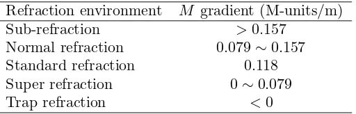
where k is the trapping layer slope and h the duct height. The modified refractivity slope above the duct height is 0.118 M-units/m, which is in accord with the standard atmosphere. In this paper, the two-linear surface ducts modified refractivity profile model is adopted as the ducting profile model.
The propagation track of electromagnetic wave is mainly determined by M gradient. When
340 350 360 370 380 390 0
50 100 150 200 250 300
Modified Refractivity (M-units)
H
e
ig
ht
(m
)
h k
0.118 M-units/m
Figure 1. Two-linear surface ducts modified refractivity profile.
Table 1. M gradient and refraction environment.
Refraction environment M gradient (M-units/m)
Sub-refraction >0.157
Normal refraction 0.079∼0.157
Standard refraction 0.118
Super refraction 0∼0.079
Trap refraction <0
3. DOPPLER WEATHER RADAR ECHOES CALCULATION
Considering a refractivity structure in a maritime environment, the expected clutter power is obtained based on the radar function and environmental parameters. For the Doppler weather radar, the radar equation [52] is
P = Pt (4π)3R4G
2λ2σ (6)
where Pt is the radar transmitter power, G the radar antenna gain, σ the radar cross section, λ the
wavelength andR the distance between radar and surface targets.
Based on the radar equation, for the surface targets, assuming that the electromagnetic wave hits the surface at single grazing angle at range R, the received radar power [53] is
P =PtG24πAσ0/
L2λ2 (7)
The radar resolution cell area is
A=Rθhcτ /(2 cosφ) (8)
where σ0is the ground and sea scattering coefficient, to overcome the problem of uncertainty of σ0, geometrical ray tracing and rank correlation was used for inversion of surface ducts. L is the path loss of electromagnetic wave of Doppler weather radar, θh the antenna horizontal beam width, c the light
speed, τ i the pulse width andφ the grazing angle.
For Doppler weather radar, the radar parameter is shown in Table 2.
Doppler weather radar is an active sensor: it emits short pulses of microwave energy and measures the power scattered back by particles in the volume illuminated by its beam. Assuming that the particles are spherical and small compared to the radar wavelength, the power is related to the radar equivalent reflectivity factor. The equivalent reflectivity factor [53] can be calculated by echo powers and distance as follows:
Ze = R2P/C (9)
C = π 3P
tG2θhθvl
1024 (ln 2)λ2 |K|
2 (10)
where θh is the antenna horizontal beam width, θv the antenna vertical beam width, l/2 the radar
Table 2. Radar parameters.
Frequency (GHz) 3.0
Antenna elevation (deg.) 0.57
Antenna height (m) 169
Transmit power (kW) 700
Antenna gain (dB) 45
Antenna horizontal beam width (deg.) 1.0
Antenna vertical beam width (deg.) 1.0
Pulse width (µs) 1.0
equivalent reflectivity factor (when the Rayleigh scattering not holds), which not only depends on the size and shape of the particles, but also depends on the number of particles per unit volume and the permittivity. |K|2 is a factor function of the dielectric constant of the particles and is related to the electrical parameters of the particles. The Water ball’s values of|K|2 for S, C and X band radar are all about 0.93.
4. THE MODIFIED REFRACTIVITY PROFILE MODELING FOR HORIZONTAL INHOMOGENEOUS TROPOSPHERIC DUCTS
The tropospheric modified refractivity profile is inhomogeneous in the vertical and horizontal direction, and this inhomogeneity is conducive to calculate echo powers, which affects the inversion of atmosphere modified refractivity profile. The best modeling method for horizontal inhomogeneity is full space model of M profile parameters. The method defines the degrees of freedom for all the vertical M profile parameters in different ranges to realize the fine description of atmosphere refractivity structure. Because the number of horizontal degrees of freedom is too many, a dimension reduction method for horizontal inhomogeneity modeling is needed, and the PCA method [54, 55] based on K-L transformation can remove the relativity among every component of original high-dimension random variable, and then remove these dimensions including little information to obtain a low-dimension coordinate system.
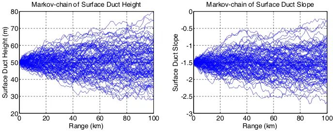
In this method, two parameters, duct height and trapping layer slope, are used to describe surface ducts, and the two parameters are generated by Markov-chain [56–58] simulation:
H = [h1, h2,· · ·] K = [k1, k2,· · ·] (11)
h1 = h0 k1=k0 (12)
hi+1 = hi+ηi ki+1=ki+ωi (13)
ηi ∼ N0, ση2 ωi ∼N0, σ2ω (14)
where h0 and hi respectively represent the surface duct height in initial range step and the number i range step;k0 and ki respectively represent the surface ducts trapping layer slope in initial range step and the number i range step; η is Gauss distribution random variable whose average value is 0, and variance isση2;ωis also Gauss distribution random variable whose average value is 0, and variance isσ2ω. The multidimensional random variables H and K respectively form a Markov-chain. A large number of simulated Markov-chains form the sample matrixes of horizontal inhomogeneous surface duct height and trapping layer slope.
The covariance matrix is calculated based on the sample matrix formed by Markov-chains. Then its eigenvalue and eigenvector are decomposed, and these eigenvectors correspond to larger eigenvalues form the principal components of surface ducts profile parameters.
The sample matrix formed by Markov-chain simulation is
M =
⎛ ⎜ ⎜ ⎝
x11 x12 · · · x1n x21 x22 · · · x2n
..
. ... ...
xm1 xm2 · · · xmn
⎞ ⎟ ⎟
The covariance matrix of the sample matrix is assumed asC, andQis an orthogonal matrix meets the condition:
C =QΛQT (16)
where Λ is the eigenvalue matrix and Q the eigenvector matrix. The larger k eigenvalues [59] are assumed as
λ1≥λ2 ≥ · · ·λk (17)
The k eigenvectors corresponding to the k eigenvalues are called as principle components, which form a new eigenvector matrix. We can choose a certain number eigenvectors based on actual condition. The number of principal components depends on the cumulative contribution rate of eigenvalues. For
example, assuming that it is 95%, when
t
i=1 λi/
k
j=1
λj ≥0.95,t is the number of principal components.
The surface duct height and trapping layer slope are represented by these above principle components:
h(r, c1, c2,· · · , cn) = h0+
n
i=1
civi(r) (18)
k(r, d1, d2,· · ·, dn) = k0+
n
i=1
diμi(r) (19)
wherenis the number of eigenvectors;vi(r) andμi(r) are the eigenvectors; ci anddi are the coefficients of corresponding eigenvectors. The Markov-chains of surface duct height and trapping layer slope are shown in Fig. 2. In this paper,ση = 1.0,σω= 0.05 andh0= 50,k0 =−1.5; the number of Markov-chain samples is 1000. Once h and kis obtained, the modified refractivity profile will be obtained according to Eq. (5).
0 20 40 60 80 100
20 30 40 50 60 70 80
Range (km)
S
u
rf
ace D
u
c
t
H
e
ig
ht
(m
)
Markov-chain of Surface Duct Height
0 20 40 60 80 100
-3 -2.5 -2 -1.5 -1 -0.5 0
Range (km)
S
u
rf
ace Duc
t S
lope
Markov-chain of Surface Duct Slope
Figure 2. Markov-chain of surface duct height and trapping layer slope.
5. PSO ALGORITHM OF RETRIEVING SURFACE DUCTS BY DOPPLER WEATHER RADAR ECHOES
The method of retrieving horizontal inhomogeneous tropospheric ducting M profile is varied. This paper firstly retrieves horizontal principal component coefficient of profile parameters, then obtains all space M profile structure based on these coefficients. The surface duct height and trapping layer slope all have two principle components and corresponding coefficients. So six profile parameters (h0, c1, c2, k0, d1, d2) are needed to retrieve to obtain all space M profiles.
It is assumed that the space dimension of solutions isn; the number of particles ism; the position of every particle is presented as Zi = (zi1, z2,· · ·, zin), the speed of the particle as Vi = (vi1, vi2,· · · , vin), the best position of the particle as Pi = (pi1, pi2,· · ·, pin), and the best position of all the particles as Pg = (pg1, pg2,· · · , pgm). The updating of speed and position of particles are presented as
vgij+1 = ξvijg +l1ug1
pgij −zgij
+l2ug2
pggj−zijg
(20)
zgij+1 = zgij+vgij+1 (21)
where i= 1,2,· · ·, m,j = 1,2,· · · , n, g is the number of evolution generations;ξ is the inertia factor;
l1,l2 are learning factors;u1, u2 between [0,1] are random numbers which keep the variety of the group. The particles move according to Eqs. (20) and (21) until meet the conditions. The settings of PSO searching parameters are: the number of particles is 100; the number of evolution generations is 20.
The PE method is widely used in acoustics and wireless propagation [60], and the parabolic equation is obtained through wave equation, which is very suitable for solving wireless propagation in atmospheric ducts [61]. An objective function is adopted for judging the difference between simulated and measured clutter power. The objective function [47] is:
f(m) =
Rm
R=R0
g2(R) (22)
where R0 represents the minimum receive range of radar clutter, Rm the maximum receive range of radar clutter andg(R) the difference between simulated and measured clutter power.
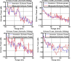
Through the PSO algorithm, the six best parameters of refractivity profile are obtained. It is assumed that they are hbest, c1, c2, kbest, d1, d2, so the modified refractivity profile will be obtained according to Equation (5). According to PE method of electromagnetic wave propagation and the inversion modified refractivity profile, the inversion echo powers is obtained and shown in Fig. 3.
In Fig. 3, inversion and measured powers of four azimuths (90 deg, 120 deg, 150 deg, and 180 deg) are shown. The blue line represents the inversion echo powers by PSO algorithm, and the red line represents the measured echo powers in 18th July, 2014. The area distribution of inversion and measured echo
20 40 60 80
-105 -100 -95 -90 -85 Range (km) E c hoes P o w e r (d B )
Echoes Power (Azimuth=150deg)
Inversion Echoes Power Measured Echoes Power
20 40 60 80
-105 -100 -95 -90 -85 -80 Range (km) E c hoes P o w e r (dB )
Echoes Power (Azimuth=180deg)
Inversion Echoes Power Measured Echoes Power
20 40 60 80
-90 -85 -80 -75 -70 -65 Range (km) Ec h o e s Po w e r ( d B )
Echoes Power (Azimuth=90deg)
Inversion Echoes Power Measured Echoes Power
20 40 60 80
-110 -100 -90 -80 -70 Range (km) E c hoes P o w e r (d B )
Echoes Power (Azimuth=120deg) Inversion Echoes power Measured Echoes Power
Figure 4. Area distribution of inversion and measured echo powers.
Figure 5. Area distribution of inversion and measured Ze.
powers are shown in Fig. 4, and the inversion range is between 10 km and 80 km. The north direction is set as the initial azimuth, so the inversion azimuth is from 80 deg to 180 deg. The error of echo powers is basically between −5 and 5 dB, which indicates that the inversion power coincides well with the measured power, especially in the increasing and decreasing point of echo powers, and the accuracy is helpful for retrieving the surface ducts modified refractivity profile.
Then the equivalent reflectivity factor is obtained based on the calculated echo powers. The area distribution of inversion and measured equivalent reflectivity factor is shown in Fig. 5, which shows that the reflectivity factor is larger from 80 deg to 110 deg azimuths than that in other azimuths. The error of equivalent reflectivity factor is between−5 and 5 dB, which indicates the accuracy of this method.
Through the comparison of echo powers in different azimuths, the echo powers are larger, in 80 deg to 120 deg, than other azimuths, so it indicates that higher duct heights exist in these areas, which is proved in Fig. 6 and Fig. 7. In every azimuth direction, the echo powers decrease with the range.
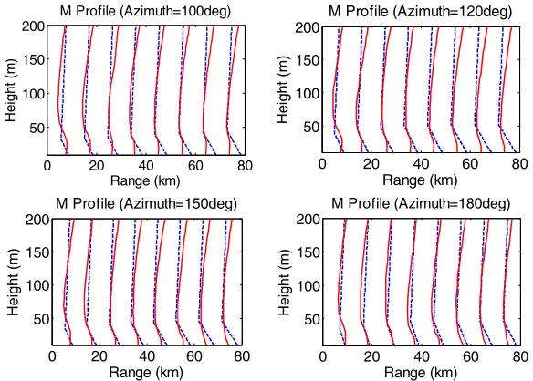
The inversion surface duct height and trapping layer slope are in the following, which includes four azimuths: 90 deg, 120 deg, 150 deg and 180 deg.
basically accord with measured M profiles when azimuth equals 150 deg or 180 deg, and the inversion precision is not very good when azimuth equals 100 deg or 120 deg, which is probably caused by radar performance or weather factors. As a whole, it indicates the validity of this inversion method.
In the standard atmosphere, the area distribution of echo powers and equivalent reflectivity factor are shown is Fig. 8. In the standard atmosphere, the echo powers decreases faster than that in surface ducts, which causes the faster decrease of the equivalent reflectivity factor. In the surface ducts, the radar electromagnetic wave is trapped in the ducts layer, which forms over-the-horizon propagation so that the echo powers will decrease slower than that in the standard atmosphere.
The modified refractivity varies with the range and different azimuths, which reflects its inhomogeneity in vertical and horizon direction. It is basically the same above the duct height, but the modified refractivity below the duct height has a serious effect on the electromagnetic wave propagation so that it forms anomalous propagation.
0 50 100 45 50 55 60 Azimuth=90deg Range (km) D u c t H e ight (m )
0 50 100 -2.5 -2 -1.5 -1 Range (km) Slope (M -unit s/m)
0 50 100 30 40 50 60 Azimuth=120deg Range (km) D u c t H e ight (m )
0 50 100 -2.5 -2 -1.5 -1 Range (km) Slope (M -uni ts/m)
0 50 100 30 40 50 Azimuth=150deg Range (km) Du c t He ig h t (m )
0 50 100 -2.5 -2 -1.5 -1 Range (km) Sl ope ( M -u ni ts/m )
0 50 100 30 40 50 Azimuth=180deg Range (km) D u c t H e ight (m )
0 50 100
-2 -1 0 Range (km) S lope ( M -u ni ts /m )
Figure 6. Inversion duct height and slope distribution with range in four azimuths (90 deg, 120 deg, 150 deg and 180 deg).
0 20 40 60 80
50 100 150 200
M Profile (Azimuth=100deg)
Range (km) He ig h t ( m )
0 20 40 60 80
50 100 150 200
M Profile (Azimuth=120deg)
Range (km) He ig h t ( m )
0 20 40 60 80
50 100 150 200
M Profile (Azimuth=150deg)
Range (km) H e ight ( m )
0 20 40 60 80
50 100 150 200
M Profile (Azimuth=180deg)
Range (km) He ig h t ( m )
20 40 60 80 -80
-60 -40 -20 0
Range (km)
R
a
ng
e (
k
m)
Echoes Power of Standard Atmosphere (dB)
-130 -120 -110 -100 -90 -80 -70 -60
20 40 60 80
-80 -60 -40 -20 0
Range (km)
R
a
ng
e (
k
m)
Ze of Standard Atmosphere (dB)
-5 0 5 10 15 20 25
Figure 8. Area distribution of echo powers and Ze for standard atmosphere.
6. ANALYSIS OF THE EQUIVALENT REFLECTIVITY FACTOR
The previous section has introduced that the equivalent reflectivity factor is different for tropospheric ducts and standard atmosphere condition. The main reason for the difference is the modified refractivity profile. In Fig. 9, four different times measured equivalent reflectivity factors within a range of 200 km are shown, which indicate that the equivalent reflectivity factor changes with the time.
In 08:01, the maritime equivalent reflectivity factor exists within a range of 20 km, but in 12:04, the maritime equivalent reflectivity factor exists beyond a range of 100 km, which indicates that in 08:01, the atmosphere condition is close to standard atmosphere and that in 12:04, the tropospheric ducts exist over the sea. It is concluded that the tropospheric ducts change with time, and the variety of ducts is related to the modified refrativity profile. Through the area distribution of the equivalent reflectivity factor, the atmosphere condition and refractivity environment are basically clear for us. The data quality of the Doppler weather radar is important for the detection of the atmosphere and targets. The inversion of the torposphere ducts modified refractivity profile also depends on the data quality of the Doppler weather radar.
The Doppler weather radar echoes are affected by multiple factors such as meteorology factors. Fig. 10 shows four times (06:00, 08:00, 10:00, 12:00) wind speed distribution based on mesoscale WRF
Figure 10. Wind speed distribution.
model. It is indicated that the wind speed is less than 7 m/s and the Douglas sea state grade less than 2. The wind speed has little effect on Doppler weather radar echoes, which indicates that the anomalous propagation is related to the vertical and horizontal inhomogeneities of the modified refractivity.
7. CONCLUSION
The tropospheric ducts have a serious effect on the propagation of the electromagnetic wave, which causes anomalous propagation. The refractive index which is inhomogeneous in both vertical and horizontal directions can be effectively used to describe the atmospheric condition, and it is badly needed to obtain the distribution of the refractivity profiles. This paper retrieves the surface ducts modified refractivity profile by Doppler weather radar echoes based on PE method for calculating electromagnetic wave propagation and PSO algorithm for searching optimal solution. The PCA method is used to model modified refractivity profile considering the horizontal inhomogeneity of the refractivity profile.
ACKNOWLEDGMENT
The authors gratefully acknowledge supports from the National Natural Science Foundation of China under Grant No. 41205024 and 41305024.
REFERENCES
1. Bech, J., B. Codina, and J. Lorente, “Forecasting weather radar propagation conditions,” Meteorology and Atmospheric Physics, Vol. 96, No. 3–4, 229–243, 2007.
2. Lakshmanan, V., A. Fritz, T. Smith, K. Hondl, and G. Stumpf, “An automated technique to quality control radar reflectivity data,” Journal of Applied Meteorology and Climatology, Vol. 46, No. 3, 288–305, 2007.
3. LeFurjah, G., R. Marshall, T. S. Casey, T. Haack, and D. De Forest Boyer, “Synthesis of mesoscale numerical weather prediction and empirical site-specific radar clutter models,” IET Radar, Sonar and Navigation, Vol. 4, No. 6, 747–754, 2010.
4. Park, S. and F. Fabry, “Estimation of near-ground propagation conditions using radar ground echo coverage,” Journal of Atmospheric and Oceanic Technology, Vol. 28, No. 2, 165–180, 2011.
5. Rico-Ramirez, M. A. and I. D. Cluckie, “Classification of ground clutter and anomalous propagation using dual-polarization weather radar,” Ieee Transactions on Geoscience and Remote Sensing, Vol. 46, No. 7, 1892–1904, 2008.
6. Jiang, Y., L.-P. Liu, and W. Zhuang, “Statistical characteristics of clutter and improvements of ground clutter identification technique with doppler weather radar,” Journal of Applied Meteorological Science, Vol. 20, No. 2, 203–213, 2009.
7. Qin, J., R.-B. Wu, Z.-G. Su, and X.-G. Lu, “Ground clutter suppression in airborne weather radar via terrain visibility analysis,” Journal of Electronics & Information Technology, Vol. 34, No. 2, 351–355, 2012.
8. Villarini, G. and W. F. Krajewski, “Review of the different sources of uncertainty in single polarization radar-based estimates of rainfall,” Surveys in Geophysics, Vo. 31, No. 1, 107–129, 2010.
9. Bech, J., U. Gjertsenb, and G. Haasec, “Modelling weather radar beam propagation and topographical blockage at northern high latitudes,”Quarterly Journal of the Royal Meteorological Society, Vol. 133, No. 626A, 1191–1204, 2007.
10. Roy Bhowmik, S. K., S. S. Roy, K. Srivastava, et al., “Processing of Indian Doppler Weather Radar data for mesoscale applications,”Meteorology and Atmospheric Physics, Vol. 111, No. 3–4, 133–147, 2011.
11. Charalampidis, D., T. Kasparis, and W. L. Jones, “Removal of nonprecipitation echoes in weather radar using multifractals and intensity,” Ieee Transactions on Geoscience and Remote Sensing, Vol. 40, No. 5, 1121–1131, 2002.
12. Chen, C.-N., J.-L. Wang, C.-M. Chu, and F.-C. Lu, “Ray-trace of an abnormal radar echo using geographic information system,”Defence Science Journal, Vol. 59, No. 1, 63–72, 2009.
13. Chang, P.-L. and P.-F. Lin, “Radar anomalous propagation associated with foehn winds induced by Typhoon Krosa (2007),” Journal of Applied Meteorology and Climatology, Vol. 50, No. 7, 1527– 1542, 2011.
14. Cho, J. Y. N. and E. S. Chornoboy, “Multi-PRI signal processing for the terminal doppler weather radar. Part I: Clutter filtering,” Journal of Atmospheric and Oceanic Technology, Vol. 22, No. 5, 575–582, 2005.
15. Da Silveira, R. B. and A. R. Holt, “An automatic identification of clutter and anomalous propagation in polarization-diversity weather radar data using neural networks,”Ieee Transactions on Geoscience and Remote Sensing, Vol. 39, No. 8, 1777–1788, 2001.
17. Fornasiero, A., J. Bech, and P. P. Alberoni, “Enhanced radar precipitation estimates using a combined clutter and beam blockage correction technique,” Natural Hazards and Earth System Sciences, Vol. 6, No. 5, 697–710, 2006.
18. Hubbert, J. C., M. Dixon, and S. M. Ellis, “Weather radar ground clutter. Part II: Real-time identification and filtering,”Journal of Atmospheric and Oceanic Technology, Vol. 26, No. 7, 1181– 1197, 2009.
19. Grecu, M. and W. F. Krajewski, “Detection of anomalous propagation echoes in weather radar data using neural networks,” IEEE Tran. Geosc. Remote Sens., Vol. 37, 287–296, 1999.
20. Grecu, M. and W. F. Krajewski, “An efficient methodology for detection of anomalous propagation echoes in radar reflectivity data using neural networks,”J. Atmos Oceanic Technol., Vol. 17, 121– 129, 2000.
21. Moszkowicz, S., G. J. Ciach, and W. F. Krajewski, “Statistical detection of anomalous propagation in radar reflectivity patterns,” Journal of Atmospheric and Oceanic Technology, Vol. 11, No. 4, 1026–1034, 1994.
22. Zhao, R. J. and G. L. Wen, “Analysis on the two cases of atmospheric duct and CINRAD/SA super-refraction echoes,”Scientia Meteorologica Sinica, Vol. 30, No. 3, 393–401, 2010.
23. Berenguer, M., D. Sempere-Torres, C. Corral, et al., “A fuzzy logic technique for identifying nonprecipitating echoes in radar scans,” Journal of Atmospheric and Oceanic Technology, Vol. 23, No. 9, 1157–1180, 2006.
24. Zhang, J.-P., “Methods of retrieving tropospheric ducts above ocean surface using radar sea clutter and GPS signals,” Xidian University, Xi’an, 2012.
25. Tabrikian, J. and J. L. Krolik, “Theoretical performance limits on tropospheric refractivity estimation using point-to-point microwave measurements,”IEEE Trans. Antennas Propag., Vol. 47, No. 11, 1727–1734, 1999.
26. Barrios, A., “Estimation of surface-based duct parameters from surface clutter using a ray trace approach,”Radio Sci., Vol. 39, RS6013, 2004.
27. Sengupta, N. and I. A. Glover, “Refractivity and humidity profiling using wind profiler and microwave radiometer observations for the inference of radio ducts,” Proc. of URSI General Assembly, New Delhi, India, 2005.
28. Valtr, P. and P. Pechac, “Novel method of vertical refractivity profile estimation using angle of arrival spectra,” Proc. of 28th General Assembly of International Union of Radio Science, New Delhi, India, 2005.
29. Cheong, B. L., R. D. Palmer, C. D. Curtis, et al., “Refractivity retrieval using the phased-array radar: first results and potential for multimission operation,” IEEE Trans. Geosci. Remote Sens., Vol. 46, No. 9, 2527–2537, 2008.
30. Park, S. and F. Fabry, “Estimation of near-ground propagation conditions using radar ground echo coverage,” J. Atmos. Oceanic Technol., Vol. 28, No. 2, 165–180, 2011.
31. Wang, H.-G., “Method and experiment of tropospheric ducts inversion using ground-based GNSS occultation,” Xidian University, Xi’an, 2013.
32. Wang, B., “Method and experiment of tropospheric ducts inversion using radar sea clutter and GNSS,” Xidian University, Xi’an, 2011.
33. Lakshmanan, V., J. Zhang, K. Hondl, et al., “A statistical approach to mitigating persistent clutter in radar reflectivity data,” IEEE Journal of Selected Topics in Applied Earth Observations and Remote Sensing, Vol. 5, No. 2, 652–662, 2012.
34. Delrieu, G., S. Caoudal, J. D. Creutin, “Feasibility of using mountain return for the correction of ground-based X-band weather radar data,” J. Atmos. Ocean Tech., Vol. 14, 368–385, 1997. 35. Cheong, B. L. and R. D. Palmer, “A time series weather radar simulator based on high-resolution
atmospheric models,” Journal of Atmospheric and Oceanic Technology, Vol. 25, No. 2, 230–243, 2008.
Vol. 47, No. 11, 1949–1957, 2011.
37. Krajewski, W. F. and B. Vignal, “Evaluation of anomalous propagation echo detection in WSR-88D data: A large sample case study,” Journal of Atmospheric and Oceanic Technology, Vol. 18, No. 5, 807–814, 2001.
38. Mesnard, F. and H. Sauvageot, “Climatology of anomalous propagation radar echoes in a coastal area,”Journal of Applied Meteorology and Climatology, Vol. 49, No. 11, 2285–2300, 2010.
39. Pamment, J. A. and B. J. Conway, “Objective identification of echoes due to anomalous propagation in weather radar data,” Journal of Atmospheric and Oceanic Technology, Vol. 15, No. 1, 98–113, 1998.
40. Seo, B.-C., W. F. Krajewski, A. Kruger, P. Domaszczynski, and J. A. Smith, “Matthias steiner,” Journal of Hydroinformatics, Vol. 13, No. 2, 277–291, 2011.
41. Sheikh, A. U. H., P. Z. Khan, and S. A. Al-Semari, “A study of anomalous propagation in persian gulf,”Ieee Transactions on Antennas and Propagation, Vol. 58, No. 6, 2029–2036, 2010.
42. Villarini, G. and W. F. Krajewski, “Sensitivity studies of the models of radar-rainfall uncertainties,” Journal of Applied Meteorology and Climatology, Vol. 49, No. 2, 288–309, 2010.
43. Zhuang, X., S. Hu, F. Xu, D. Hu, and Q. Liang, “Application of an automated algorithm to remove anomalous propagation ground returns in nowcasting,”Scientia Meteorologlca Sinica, Vol. 29, No. 2, 241–245, 2009.
44. Bebbington, D., S. Rae, J. Bech, B. Codina, and M. Picanyol, “Modelling of weather radar echoes from anomalous propagation using a hybrid parabolic equation method and NWP model data,” Natural Hazards and Earth System Sciences, Vol. 7, No. 3, 391–398, 2007.
45. Bech, J., B. Codina, J. Lorente, and D. Bebbington, “The sensitivity of single polarization weather radar beam blockage correction to variability in the vertical refractivity gradient,” Journal of Atmospheric and Oceanic Technology, Vol. 20, No. 6, 845–855, 2003.
46. Karimian, A., C. Yardim, P. Gerstoft, W. S. Hodgkiss, and A. E. Barrios, “Refractivity estimation from sea clutter: An invited review,” Radio Science, Vol. 46, 2011.
47. Zhang, J.-P., “Methods of retrieving tropospheric ducts above ocean surface using radar sea clutter and GPS signals,” Xidian University, Xi’an, 2012.
48. Yang, C., L.-X. Guo, H.-Q. Li, and Z.-S. Wu, “Study the propagation characteristic of radio wave in atmospheric duct,”Journal of Xidian University, Vol. 36, No. 6, 1097–1102, 2009.
49. Dong, C., L. Li, and Z.-S. Wu., “The analysis on offshore atmospheric duct with parabolic equation method,”Electronic Sci. &Tech., Vol. 23, No. 11, 91–93, 99, 2010.
50. Zheng, Q., X.-W. Gong, and W.-H. Wu, “On application of particle filter combining with particle swarm optimization to refractivity estimation from radar clutter,” Journal of PLA University of Science and Technology (Natural Science Edition), Vol. 14, No. 3, 322–328, 2013.
51. Yao, J.-S. and S.-X. Yang, “Practical application of the Paulus-Jeske (PJ) model to the littoral,” Fire Control &Command Control, Vol. 35, No. 6, 121–124, 2010.
52. Lu, J.-Q. “Research of modeling and simulation of radar echo signal,” The PLA Information Engineering University, Zhengzhou, 2006.
53. Wang, H.-G., H. Zhang, and Z.-S. Wu, “Study of simulating anomalous ground echoes for doppler weather radar,”Journal of Electronics&Information Technology, Vol. 35, No. 12, 2863–2867, 2013. 54. Xi, X.-Y. and H. Liu, “Research on comparison of principal component analysis with independent
component analysis,” Geophysical Prospecting For Petroleum, Vol. 45, No. 5, 441–446, 2006. 55. Wang, H.-G., “Method and experiment of tropospheric ducts inversion using ground-based GNSS
occultation,” Xidian University, Xi’an, 2013.
56. Pan, F., Q. Zhou W.-X., Li, and Q. Gao, “Analysis of standard particle swarm optimization algorithm based on Markov chain,”Acta Automatica Sinica, Vol. 39, No. 4, 381–389, 2013. 57. Ren, Z.-H., J. Wang, and Y.-L. Gao, “The global convergence analysis of particle swarm
58. Guo, H.-K., J. Wu, Z.-F. Ying, and X. Lu, “A special kind of random sequences’ improved Markov chain modeling,”Academic Conference of the Sixteenth National Youth Communication, 2011. 59. Zhao, J.-F. and X.-H. Chen, “Dual optimization of seismic attributes based on principle component
analysis and K-L transform,”Geophysical&Geochemical Exploration, Vol. 29, No. 3, 253–256, 2005. 60. Levy, M., Parabolic Equation Methods for Electromagnetic Wave Propagation, Institution of
Electrical Engineers, London, 2000.