An Exactly-Solvable Quasistatic Electricity Inverse Problem:
Retrieval of the Complex Permittivity of a Cylinder Taking Account
of Nuisance Parameter Uncertainty
Armand Wirgin*
Abstract—This study concerns the 2D inverse problem of the retrieval, using external field data, of either one of the two physical parameters, constituted by the real and imaginary parts of the permittivity, of a z-independent cylindrical dielectric specimen subjected to an external, z-independent, quasistatic electric field. Six other parameters enter into the inverse problem. They are termed nuisance parameters because: 1) they are not retrieved during the inversion and 2) uncertainty as to their actual values can adversely affect the accuracy of the retrieval of the permittivity. This inverse problem is shown to have an exact, mathematically-explicit, solution, both for continuous and discrete input data, whose properties, with respect to the various nuisance parameter uncertainties, are analyzed for noiseless data. It is found that: a) optimal inversion requires data registered at only a small number of sensors, b) the inverse solution, satisfying pre-existing physical constraints, exists and is unique. Moreover, the inverse solution is shown to be unstable with respect to three nuisance parameter uncertainties, the consequence of which is large retrieval inaccuracy for small nuisance parameter uncertainties, acting either individually or in combination.
1. INTRODUCTION
The retrieval of the complex permittivity (or related physical parameters such as the dielectric constant, index of refraction, absorption coefficient, . . .) of a homogeneous, isotropic material is a theoretical and experimental electromagnetic inverse (although only relatively-recently recognized as such) problem of considerable importance. The reason for this is that permittivity is a sensitive indicator of the chemical [2] and physical identity of natural and man-made materials [17] and of their state (notably in quality control and health monitoring [21] applications) [19, 22].
The usual techniques (comparison of capacities, resonant circuits, transmission lines, dielectrometry, reflectometry, refractometry, ellipsometry) rely (to match theory to measurement) on the possibility of obtaining homogeneous specimens of prescribed (usually-simple) shape (often blocks, cylinders, spheres, slabs) and size (e.g., films). In naturally-occurring materials, this is not always possible. For instance, in studies of natural phenomena connected with the scattering of light (interstellar dust, air-borne pollution, powders, granular media and other divided matter characterizations, material characterization of living bodies (cells, phytoplancton, etc.), the specimens can have complicated shapes (although they are often considered to be spherical or cylindrical [3, 6]) and are too small (e.g., films so thin that the matter therein appears to be divided) to be examined by the previously-mentioned techniques [3, 6, 14, 20]. It is thus increasingly recognized that discrepancies between the assumed and actual: size, shape and composition of the specimen (divided versus homogeneous, such as in colloids and metamaterials [4, 5, 18]) have to be taken into account in connection with the meaning
Received 16 November 2014, Accepted 16 December 2014, Scheduled 26 December 2014
* Corresponding author: Armand Wirgin ([email protected]).
that is attached to the permittivity determined from the response of the specimens to quasistatic or dynamic (wave-like) electric fields (the latter response incorporates diffraction and/or collective effects, not ordinarily accounted-for in methods relying on reflective or refractive response fields). A second trend of permittivity retrieval inverse problems is the recognition of the necessity of taking into account the uncertainty (of the experimental results [20]) of certain parameters (and their sensitivity [5]) that enter into the retrieval model, and of the mathematical ingredients of the retrieval model itself [15], in order to evaluate the accuracy of the retrieved parameters, e.g., [7, 9, 10, 20]. The present investigation is inspired by these two trends.
We shall be concerned with an isotropic, generally-inhomogeneous, lossy dielectric medium in which the displacement and the conduction current density are related to the electric field by a dielectric constant ε(x, ω) and loss factor ε(x, ω) respectively via the constitutive relations:
D(x, ω) =ε(x, ω)E(x, ω), Jc(x, ω) =ωε(x, ω)E(x, ω), (1) wherein: ω is the angular frequency (Hz), x a position vector, andε and ε are generally (for passive media) positive (or zero) scalar functions for ω ≥ 0. In the quasistatic regime and in the absence of impressed bulk charges, it ensues (also fromE=−∇ψ,ψ the quasistatic electric potential) that
∇ ·[ε(x, ω)∇ψ(x, ω)] = 0, (2) whereinε(x, ω) =ε(x, ω) +iε(x, ω) is the (complex) permittivity. Henceforth, we drop the symbolω, considered to be implicit.
Let Rn be divided into two domains D0 and D1, separated by the interface I, the unit vector
normal to which is ν. Let M0 and M1 be two homogeneous, isotropic dielectric media (fillingD0 and
D1 respectively) in which the position-independent permittivities areε0 and ε1, respectively.
If all space (i.e.,D0+D1) is initially occupied solely byM0 and devoid of impressed charges, but
subjected to a uniform electric field Ei satisfying Ei(x) = −∇ψi(x), then the introduction of M1 into
D1 induces a potential ψd0 inD0 so that the total potentials are now
ψ0(x) =ψi(x) +ψ0d(x) inD0, ψ1(x) =ψd1(x) inD1. (3)
Then the problem of the prediction of ψl; l= 0,1, for givenEi orψi, can be cast in the three-relation
form (equivalent to (2))
∇ ·(∇ψl)(x) = 0 inDl, l= 0,1, (4)
ψ0(x)−ψ1(x) = 0 on I, (5)
ε0(x)ν(x)· ∇ψ0(x)−ε1(x)ν(x)· ∇ψ1(x) = 0 onI, (6)
with uniqueness assured by the condition:
ψld(x)<∞ inDl; l= 0,1. (7)
In the preceding lines, the emphasis has been on the forward problem of the prediction of the potential fieldψ, assuming that all other ingredients of the configuration and of the solicitation (viaψi) are known. Actually, the present investigation is more specifically concerned with theinverse problem
(examples of which can be found in [1, 6, 7, 9–11, 13, 16]) of the retrieval of ε(or, more precisely, ofε1)
from data relative toψ(more precisely, ψ0), assuming that all other parameters of the configuration as
well as of the solicitation (i.e., the nuisance parameters [7]) are more or less well-known (i.e., uncertain to some degree). We qualify a parameter as being uncertain by the fact that its assigned value, resulting from experiment, guessing or borrowing from a published result, is incorrect in a sense akin to systematic measurement error.
The chosen physical configuration (in whichD1is an infinitely-long circular cylinder) will be shown
2. DESCRIPTION OF THE PHYSICAL CONFIGURATION
A circular cylinder, occupied by the homogeneous, isotropic medium M1 (in which the permittivity is
ε1) is introduced into another homogeneous, isotropic mediumM0 (in which the permittivity is ε0) of
infinite extent and is submitted to an electric fieldEi whose direction is assumed to be constant at all points of space. Thezaxis (of the cartesian coordinate systemOxyzforms the axis of the cylinder and the circular disk Ω1, with center at O, constitutes the support of the cylinder in the x-y plane. The
unbounded region exterior to Ω1 (in thex-y plane) is Ω0.
The incident electric field vector Ei is assumed to lie in the x-y plane and independent of z. The circular boundary of Ω1 is Γ, the outward unit vector normal to which isν. Consequently, the incident
and induced fields are independent of z, i.e., the problem is two-dimensional, with z the ignorable coordinate. In the so-called forward problem, the task is to predict the secondary field Ed = −∇ψd induced by the primary field Ei =−∇ψi, whereas in the inverse problem, the associated potential ψd (combined withψi) constitutes the data, which, by means of an inversion scheme, is analyzed to enable the retrieval of the constitutive parameter ε1 of M1. The units of E, ψ, ε, a,θi, b and θ are: volt/m,
volt, farad/m, m, ◦ or rad, m,◦ or rad respectively.
With r, θ the polar coordinates of a point P in the x-y plane and x the vector joining O to P, the parametric equation of Γ is r = a; ∀θ ∈ [0,2π[, a being the radius of the circular disk Ω1. The
(incident) angle between Ei and the x axis is θi. The total (primary plus secondary) potential field is sensed at various points on a circle (concentric with Γ) of radius b > a. The polar angle at which a generic point-like sensor is located isθ.
The first objective is: given ei (amplitude of ψi), θi, a and εl; l = 0,1, find the total potential
fields at one or more positions (starting withθ=θb) on the circler=b. It is assumed that the location of the axis of the cylinder is known (and coincides with the z-axis) and that the number, and angular, positions of the point-like (in the x-y plane) sensors are perfectly well-known in both the forward and inverse problem contexts.
The second objective is: given the total potential fields registered at one or more sensors located at angular positions starting withθ=θb on the circler =B (analogous to, but different from,bdue to uncertainty of this parameter), as well as the set of parametersEi, Θi,A andE0 (analogous toei,θi,a
andε0, but integrating uncertainties), find (in separate steps)E1 (analogous toε1) andE1(analogous to
ε1). Actually, theexact solution (to simulate measured data concerning the total field), of the forward problem, will be employed as the data (the corresponding model is termed the data simulation model) to solve the inverse problem in the second part of the document. In addition, we appeal to aparameter retrieval model, also based on the aforementioned physical configuration, to recover the constitutive parameter of the cylinder. Some of the fixed (during the inversion) parameters (the so-called nuisance parameters) of the retrieval models will be assumed to be not precisely known, and their effect on the accuracy of the retrievals will be studied in depth.
3. EXACT SOLUTION OF THE FORWARD PROBLEM
The assumed primary electric potential is
ψi(r, θ) =−eircos(θ−θi), (8) with ei a constant amplitude term. Separating variables in (4) and applying the conditions (5)–(7), gives
ψ0(x)−ψi(x) =ψ0d(x) =ei
a2
r ε
1−ε0
ε1+ε0
cos(θ−θi), (9) which is identical to that [12, p. 1185], when θi= 0.
4. EXACT SOLUTION OF THE INVERSE PROBLEM
4.1. General Considerations
of the electric potential and the parameter retrieval model (Ψ0) of the electric potential on the circle
of radius b(which becomesB if it is uncertain) in the angular interval of observation [0,2π[. This cost functional is:
K(E1,E1) = 2π
0
ψ0(b, θ|ei, θi, a, ε0, ε1, ε1)−Ψ0(B, θ|Ei,Θi, A,E0,E1,E1) 2
dθ 2π
0
ψ0(b, θ|ei, θi, a, ε0, ε1) 2
dθ
. (10)
K is actually replaced, in the numerical context, and to account for the discrete nature of the physical sensing process, by another cost functional obtained by adopting a simple quadrature rule for the integrals:
K ≈ K(N)(E
1,E1) =
δθ
N
n=1ψ0(b, θn|ei, θi, a, ε0, ε1, ε1)−Ψ0(B, θn|Ei,Θi, A,E0,E1,E1) 2
δθ
N
n=1ψ0(b, θn|ei, θi, a, ε0, ε1, ε1)
2 , (11)
whereinδθ = 2π/N, and θn=θb+δ2θ + (n−1)δθ are the actual angles (forn= 1,2, . . . , N;θb a chosen
starting angle and θe a chosen ending angle) at which the electric potential is sensed.
Note that the set of parameters (lower case letters and symbols) is different in the simulated data model from the corresponding set (upper case letters and symbols) in the parameter retrieval model; this expresses the fact that the subset of nuisance parameters (all the parameters except ε1) may be
not well known to us before and during the inversion. The fact that
ψ0(b, θ) =f(ei, a, b, ε0, ε1, ε1) cos(θ−θi), Ψ0(B, θ) =F(Ei, A, B,E0,E1,E1) cos(θ−Θi), (12)
leads to:
K(E1) =
2π
0
fcos(θ−θi)−Fcos(θ−Θi)2dθ 2π
0
fcos(θ−θi)2dθ
. (13)
and
K(N)(E 1) =
δθ
N
n=1fcos(θn−θi)−Fcos(θn−Θi)
2
dθ
δθ
N
0 fcos(θn−θi)
2
dθ
. (14)
WithGany one of the capital-letter parameters and κ= cos(Θi−θi), (13) leads to
K(G) = f
2−2κ (f∗F) +F2
f2 , (15)
wherein the symbol ∗ designates the complex conjugate operator. An extremum of the cost functional with respect to the variable G(henceforth, E orE) is found for ∂K∂G(G) = 0 or
∂F∗
∂G
(F−κf)− ∂F∗
∂G
(F−κf) = 0. (16)
4.2. Finding E1 of the Cylinder by Minimizing K
Equation (16) leads to thequartic equation C4E
4
1 +C3E
3
1 +C2E
2
1 +C1E1 +C0 = 0, (17)
whose coefficients are:
C3 = 2E0F A2−4E0(F B2+f g) + 2E1f h, C2=−2E02(F B2+f g) + 6E0E1f h, (18)
C1 = −2E0k+F A2−2E0(k++k−)(F B2+f g) + (2k++ 4E02)E1f h, (19)
wherein
k± :=E02± E12, F := E
i
B , f := eiκ
b , g:=−b
2+a2
ε12+ε12−ε20
ε1+ε02
, h:= 2a
2ε 1ε0
ε1+ε02
, (21)
It ensues that:
C1 =
2E0C0
k+
+k+(C3−2E0C4), C2 = C0
k+
+ 2E0(C3−2E0C4) +k+C4, (22)
so that the quartic equation can re-written as (E12+ 2E0E1 +k+)
C4E1(E1 −2E0) +C3E1 +
C0
k+
= 0. (23)
The solutions of ( ) = 0 are:
E(1)
1 =−E0−iE1, E
(2)
1 =−E0+iE1, (24)
whereas the two roots of [ ] = 0 are:
E(±) 1 =
−k+(C3−2E0C4)±
k2
+(C3−2E0C4)2−4k+C4C0
2k+C4
. (25)
Eqs. (24)–(25) represent the exact solutions of the inverse problem of the identification of the sole parameterE1. Recall that it was assumed thatE0,E1 andE1(of the same nature asε0,ε1,ε1respectively)
are positive real. Thus,E1(1) and E1(2) are not admissible solutions.
By a perturbation analysis, for small E1 and ε1, we find (neglecting terms of order E1 and ε, so thatg becomesg0=g
ε=0) that the approximate solution forE1 is
E
1 ≈ E0
F A2+F B2+f g(0)
F A2−F B2−f g(0) , (26)
which is a consequence of the unique, exact solution forE1
E
1 =
−k+(C3−2E0C4) +
k2
+(C3−2E0C4)2−4k+C4C0
2k+C4
. (27)
4.2.1. Comments on the Exact and Approximate Solutions for E1
The result embodied in (27) shows that:
1- the solution to the inverse problem of the identification of the sole parameterE1 exists, even in the presence of nuisance parameter uncertainties;
2- it is possible to obtain themathematically-explicit and exact solutionto the given inverse problem, even in the presence of nuisance parameter uncertainties;
3- this solution isuniquefor a given set of parametersε1, ε1, ε0, a, ei, θi, b,E1, E0, A, Ei, Θi, B,
subject to the assumed physical constraint (i.e., the real part of the permittivity should be positive real);
4- the accuracy of the retrieval of the real part of the permittivity (E1) is conditioned, albeit in a complex manner, by the uncertainty of the nuisance parametersE0, A, Ei,Θi, B;
The result embodied in (26) shows that
4.2.2. Preliminaries Concerning the Dependence of the Retrieval Error of E1 on the Nuisance Parameter Uncertainties
Due to the fifth comment in Section 4.2.1 it is no longer necessary to delve on the issue of the dependence of the retrieval error ofE1 on the (assumed-small) nuisance parameter E1. Thus, from now on, we deal with (26)
E1 =E0
ε
1X++ε0Y+
ε1Y−+ε0X−
. (28)
wherein
X± = (F A2+f a2)±(F B2−f b2), Y±= (F A2−f a2)±(F B2−f b2). (29) To unravel the complexity alluded to in the fourth comment in Section 4.2.1, first suppose that the nuisance parameters A, B, Ei,Θi are known precisely, i.e., Ei = ei, A = a, B = b, Θi = θi, whence X+=X− and Y±= 0, so that
E1 = ˇE1 =E0
ε1 ε0
, (30)
which shows that the the relative error of the retrieved parameter, i.e.,
εε1 = E
1−ε1
ε1 =
E
1
ε1 −1 =
E0−ε0
ε0
= E0 ε0
−1 :=δε0, (31)
depends linearly on the ratio E0ε
0.
4.2.3. Properties of E1 as a Function of B
We can write
E
1(B) =E0
Eib(B2+A2)−eiBM
−Eib(B2−A2)−eiBM
=−E0
⎡ ⎢ ⎢ ⎣
B2−e
iM
EibB+A
2
B2−e
iM
EibB−A
2
⎤ ⎥ ⎥
⎦:=−E0ND. (32)
wherein
M :=−κg0 =κ
(ε1+ε0)b2−(ε1−ε0)a2
ε1+ε0
. (33)
Since we assume a relatively-small uncertainty on the nuisance parameter Θi, it follows that|Θi−θi|< π/2, whence κ >0. Also, since we assume thatε0 >0,ε1>0,b2 > a2, it follows that
M >0. (34)
Finally, recall that we assume E0 >0.
Now, assume that δ >0 and considerE1(B0±δ). It is easy to show that
E
1(B0+δ) =E1(B0−δ), (35)
entails
B0 =
eiM
2Eib >0, (36)
so that
E1(B) =−E0
B2−2B0B+A2
B2−2B
0B−A2
. (37)
whence
E1(B0) =E0. (38)
Differentiating gives
dE1(B) dB =
4E0(B−B0)A2
B2−2B
0B−A2
whence
dE1(B0)
dB = 0. (40)
The equationD= 0 has two solutions
B±= eiM
Eib ±
eiM
Eib
2
+ 4A2
2 =B0±
B02+A2. (41)
at which E1 blows up.
It is generally admitted that nonlinear inverse problems are ill posed [8] which means that the solution either does not exist or is not unique (our particular inverse solution was shown to be unique when certain physical constraints are satisfied) and is unstable in the case of existence. Instability is usually defined ([1]) by retrievals not being continuously-dependent on variations of the data. We, on the other hand, find that the function E1(B) diverges at B− and B+, which suggests a new form of
instability, first observed, but not explained, in [11]. Borrowing a notion first expressed in [16], we defineretrieval instability induced by nuisance parameter uncertaintyas that which occurs when a very small variation of a nuisance parameter B (and perhaps other nuisance parameters) produces a very large variation of a retrieved parameter (at present,E1).
Now consider E1(B+±δ), with 0< δ1 defined as previously. We find
E1(B+±δ) =−E0
A2±δB20+A2
±δB02+A2
≈ ∓E0
A2
δB02+A2, (42)
which shows that for small positive δ,
E1(B+−δ)>0, E1(B++δ)<0. (43)
Similarly, for ε1,
E1(B+±ε)∼ −E0; ε→ ∞, (44)
which shows that E1(B) tends to the negative value −E0 for B → ±∞. This result, which at first
appears to be surprising since it was assumed at the outset that E1 > 0, actually means that no
physically-meaningful result can be obtained for large uncertainty of |B|. In other words,the solutions obtained for B > B+ and B < B+ must be rejected.
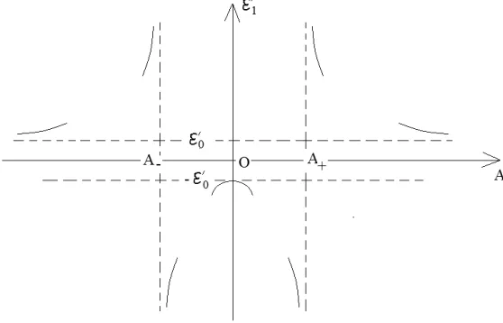
The analytical properties (symmetries, behavior in the neighborhoods of B0, B− and B+) of the
functionE1(B), deduced from the preceding formulae, are exhibited in Fig. 1.
It should be noted, in this figure, that it is possible to retrieve a physically-meaningfulE (i.e., that is positive real) only forB+> B≥0.
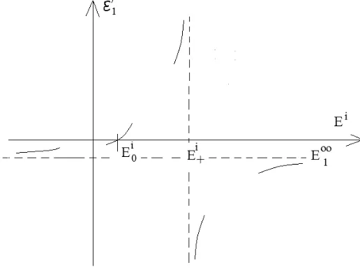
4.2.4. Properties of E1 as a Function of A
We can write
E1(A) =E0
⎡ ⎢ ⎢ ⎣
A2−e
iBM
Eib +B
2
A2−e
iBM
Eib −B
2
⎤ ⎥ ⎥ ⎦=E0
A2−C2+B2 A2−C2−B2
:=E0N
D, (45)
wherein
C2 := e
iBM
Eib (46)
The equationD= 0 has two solutions
A±=±B2−C2. (47)
at which E1 blows up.
Proceeding as in Section 4.2.3 we are able to show that the analytical properties (symmetries, behavior in the neighborhoods of A= 0, A− and A+) of the functionE1(A) are as exhibited in Fig. 2.
4.2.5. Properties of E1 as a Function of Ei
We can write
E
1(Ei) =−E0
B2+A2 B2−A2
Ei−E0i Ei−Ei
+
, (48)
wherein:
E0i = e
iBM
b(B2+A2), E
i
+ =
eiBM
b(B2−A2) > E
i
0. (49)
It ensues thatE1(Ei) blows up at Ei =Ei
+.
Proceeding as in Section 4.2.3, we can show that the analytical properties (behavior in the neighborhoods of Ei
0,E+i ) of the functionE1(Ei) are as exhibited in Fig. 3.
It should be noted, in this figure, that it is possible to retrieve a physically-meaningfulE (i.e., that is positive real) only forE+i > B > E0i.
Figure 1. Graphical representation of the analytical properties ofE1(B).
Figure 3. Graphical representation of the analytical properties ofE1(Ei).
4.2.6. Comments on the Analytical Properties of E1(A), E1(Ei), E1(B)
In Section 4.2.1, it was stated that the explicit formula for E1 demonstrates the existence of a solution of the inverse problem, even in the presence of nuisance parameter uncertainties. We now see that this statement must be interpreted in the following sense: a physically-admissible solution (i.e., positive and not infinite) for E1 exists only for a range of nuisance parameter uncertainties (i.e., those for which E1 is positive and not infinite).
Furthermore, it was stated in Section 4.2.1, that the explicit formula for E1 constitutes a unique
solution for a given set of parameters ε1, ε1, ε0, a, ei, θi, b, θb, E1, E0, A, Ei, Θi, B. However,
this does not mean that a physically-admissible E1 cannot arise from more than one sets of nuisance parameters, as is illustrated in Fig. 1 for B in the neighborhood of B0 (i.e., the two valuesB0±δ give
rise to the sameE1).
4.3. Finding the Real Part of the Permittivity of the Cylinder by Minimizing K(N)
The method of obtaining the real part of the permittivity of the cylinder outlined in Section 4.2 is somewhat unrealistic because it supposes that the data are registered at a continuum of points on the sensing circler=b. In reality, the data are registered at discrete locations on this circle, and the number N of these locations is finite. Of course,N will have an influence on the accuracy of the retrieval, and it is this influence that we shall now examine.
From (14) we obtain
K(N)(E 1) =
1
f2δ
θ N
n=1
cos2(α+ (n−1)δθ)
×δθ N
n=1
f2cos2(α+ (n−1)δ
θ)−2 (f∗F) cos(α+ (n−1)δθ) cos(β+ (n−1)δθ)
+F2cos2(β+ (n−1)δθ)
, (50)
whereinα =θb+ δθ
2 −θ
i and β =θb+δθ
2 −Θ
i, δ θ = θ
e−θb
N ,θn =θ b+δθ
2 + (n−1)δθ. Note that since
θe−θe= 2π, here we admit arbitrary θb and θb, with the only restriction thatθe> θb andθe. Consider
σ(N)(α, β) =δθ N
n=1
cosα+ (n−1)δθ
cosβ+ (n−1)δθ
, (51)
It is straightforward to show that
σ(N)(α, β) = δθ 2
Ncos(α−β) + cosα+β+ (N −1)δθ
sin(N δθ)
sin(δθ)
. (52)
and, on account of (50)
K(N)(E 1) =
|f2σ(N)(α, α)−2 (f∗F)σ(N)(α, β) +F2σ(N)(β, β)
f2σ(N)(α, α) . (53)
Forθe−θb = 2π, the fact that lim
N→∞σ
(N)(α, β) =πcos(α−β) =πcos(θi−Θi) =πκ, (54)
gives rise to the expected result
lim
N→∞K
(N)(E
1) =K(E1), (55)
Recall that our goal was to obtain an estimation ofE1 by minimizing K(N))(E1). The procedure is the same as in Section 4.2 and yields the exact (mathematical) solution
E(N) 1 =
−k+(C(3N)−2E0C4(N)) +
k+2(C(3N)−2E0C4(N))2−4k+C(4N)C (N) 0
2k+C(4N)
, (56)
and the approximate solution
E(N) 1 ≈ E0
F A2+F B2+f(N)g(0)
F A2−F B2−f(N)g(0) , (57)
wherein: C(N)
4 = F A2−(F B2+f(N)g), C (N)
3 = 2E0F A2−4E0(F B2+f(N)g) + 2E1f(N)h, (58)
C(N)
0 = −k2+F A2−k+k−(F B2+f(N)g) + 2k+E0E1f(N)h, f(N)=
eiκ(N) b , κ
(N)= σ(N)(α, β)
σ(N)(β, β).(59)
Eqs. (56)–(59) are the (mathematically) exact and approximate solutions respectively to the inverse problem for discrete data in the interval [θb + δθ
2, θ
e− δθ
2]. Eqs. (56)–(59)) show that the accuracy
of the retrieval of ε1 is conditioned, not only by the uncertainty of the nuisance parameters
E
1, E0, A, Ei, B, Θi, but also by the number N of data samples.
It is of some interest to see how the choice ofN influences the retrieval ofε1, either via the explicit formula (56) or via minimization of the cost functional K(N) in (57). To do this, we consider the case θe−θb = 2π solely, keeping in mind the reference solution obtained by minimization of the cost functional K. From (52) it ensues that
κ(N)(α, β) = cosα
cosβ; N = 1,2, κ
(N)(α, β) = cos(α−β); N ≥3, (60)
wherein
α= π N −θ
i, β= π
N −Θ
i. (61)
Consequently,
κ(1) = cosθ
i
cos Θi, κ
(2) = sinθi
sin Θi, κ
This result tells us that the retrieval depends onN for small N (= 1,2), but no longer depends onN forN ≥3, which suggests thatthe optimal number N of sensors isN = 3 separated (in terms of angle θ) by 2π/3, on the sensing circle of radius b ≥ a. Note also that owing to the result κ(N≥3) = κ, it ensues that
K(N≥3) =K, (63)
which means that the employment of the term ‘optimal’ is all the more justified that theN = 3 inversion gives rise to the reference retrieval (obtained by minimization ofK).
4.4. Finding E of the Cylinder by Minimizing K
By proceeding as in Section 4.2 we obtain the fourth-order (in terms ofE) (quartic) algebraic equation O4E
4
1 +O3E
3
1 +O2E
2
1 +O1E1+O0 = 0, (64)
wherein
O4 =f h, O3= 2
F A2(E+− E0)−(F B2+f g)E+
,
O2 = 0, O0 =−f hE+4, E±:=E1 ± E0, ε±:=ε1±ε0,
O1 = 2E+2 F A2E−−(F B2+f g)E+
+F A2E0
! ,
. (65)
It ensues from these formulae that:
O1 =E+2O3, O0=−O4E+4, (66)
so that the roots of the quartic equation can be found from
E2
1 +E+2 O4(E
2
1 − E+2) +O3E1
= 0. (67)
The two roots of ( ) = 0 are:
E(1)
1 =−iE+,
E(2) 1 =iE+
, (68)
and the two roots of [ ] = 0 are:
E(−) 1 =
−O3−
O2
3+ 4O24E+2
2O4
,
E(+) 1 =
−O3+
O2
3+ 4O24E+2
2O4
. (69)
Eqs. (68)–(69) represent the exact solutions of the inverse problem of the identification of the sole parameter E1. Recall that it was assumed that E0, E1 and E1 (of the same nature as ε0, ε1, ε1
respectively) are positive real. Thus, E1(1) and E1(2) are not admissible solutions. By a perturbation analysis, for smallE1 andε1, we find (neglecting terms of orderE1 andε1), that the approximate solution forE1 is
E
1 ≈
E2 +f h(1)
F A2−F B2−f g(0) ε, (70)
corresponding to the (only-admissible) exact solution forε1
E1 =
−O3+
O2
3+ 4O24E+2
2O4
4.4.1. Comments on the Exact and Approximate Solutions for E1
The same comments apply to the exact E1 of (71) as to the exact E1 in Section 4.2.6. The result embodied in (70) shows:
1- that the accuracy of the retrieval of E1 is strongly-conditioned by ε1 and E1 since the dependence ofE1 onε1 is linear and that on E1 is quadratic,
2- nevertheless thatE1 is usually small due toε1 having been assumed to be small,
3- that, due to the possibility of vanishing denominator in (70), the retrieval of E1, like that of E1, can be unstable with respect to the uncertainties of certain nuisance parameters.
4.5. Finding the Imaginary Part of the Permittivity (E) of the Cylinder by Minimizing
K(N)
The goal is to obtain an estimation of E1 by minimizing K(N))(E
1). The procedure is the same as in
Section 4.4 and yields the exact solution
E(N) 1 =
−O(N) 3 +
O(N)2
3 + 4O (N)2 4 E+2
2O(4N)
. (72)
and the approximate solution
E(N) 1 ≈
E2
+f(N)h(1)
F A2−F B2−f(N)g(0) ε
, (73)
wherein:
O(N)
4 =f(N)h, O (N)
3 = 2E0F A2−4E0(F B2+f(N)g). (74)
Eqs. (72) and (73) are the (mathematically) exact and approximate solutions to the inverse problem for discrete data in the interval [θb + δθ
2, θe −
δθ
2]. These relations, as well as (74), show that the
accuracy of the retrieval of E1 is conditioned, not only by the uncertainty of the nuisance parameters
E
1, E0, A, Ei, B, Θi, but also by the numberN of data samples.
As in Section 4.3, we can show that, in the caseθe−θb = 2π, the retrieval depends onN for smallN
(= 1,2), but no longer depends onN forN ≥3, which suggests thatthe optimal numberN of sensors is N = 3 separated (in terms of angle θ) by 2π/3, on the sensing circle of radius b ≥ a. Moreover, the term ‘optimal’ is all the more justified that theN = 3 inversion gives rise to the reference retrieval (obtained by minimization ofK).
5. RESULTS CONCERNING THE RETRIEVAL ERROR AS A FUNCTION OF NUISANCE PARAMETER UNCERTAINTIES
5.1. Overview of the Evaluation of Retrieval Error for Fixed Nuisance Parameter Uncertainties
All the following numerical results pertain to the choice (the true parameters of which are): ε1 = 2, ε1 = 0.1,ε0= 1, a= 0.1,ei= 1, θi = 2◦,b= 0.2. Moreover,θb = 0◦,θe= 360◦, and N = 3.
Six general cases of nuisance parameter uncertainty are possible, of which we retain only the following two:
1) one nuisance parameter is uncertain, the five others are equal to their true values;
2) five nuisance parameters are uncertain, the sixth is equal to its true value. The offered tables relate ˜E1 (or ˜E1) and EE
1 =
˜
E
1−ε1
ε1 (or EE1 =
˜
E
1−ε1
ε1 ) to δg = G−g
g for the fixed
5.2. Tables of the Influence of Uncertainty of One Nuisance Parameter, All Other Nuisance Parameters Being Certain, on the Accuracy of the Retrieval of ε1 or ε1
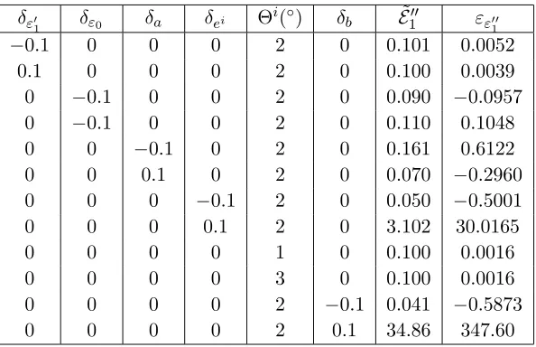
In Table 1 we give the numerical values of ˜E1 and εε1 in all of the 12 possible cases in which only one
nuisance parameter is δ=±10% uncertain at a time.
This table reveals that in six of these cases,|εε1|>|δ|, and in four of these cases, |εε1| |δ| (due
to nuisance parameter uncertainty-induced instability). In Table 2 we give the numerical values of ˜E1 and εε
1 in all of the 12 possible cases in which only
one nuisance parameter is δ=±10% uncertain at a time. This table reveals that in eight of these cases, |εε
1|> |δ|, and in seven of these cases, |εε1| |δ|
(due to nuisance parameter uncertainty-induced instability). The comparison of Table 2 with Table 1 shows that the pattern of retrieval error of E1 is substantially the same as that of E1, as previously predicted in theoretical manner.
Table 1. Retrieval ofε1 when one nuisance parameter is δ=±10% uncertain (except Θi, which when uncertain, deviates from its true value by ±1◦).
δε
1 δε0 δa δei Θ
i(◦) δ
b E˜1 εε1
−0.1 0 0 0 2 0 2.000 0.0000
0.1 0 0 0 2 0 2.000 0.0000
0 −0.1 0 0 2 0 1.800 −0.1000 0 −0.1 0 0 2 0 2.200 0.1000 0 0 −0.1 0 2 0 2.398 0.1988 0 0 0.1 0 2 0 1.761 −0.1193 0 0 0 −0.1 2 0 0.864 −0.5679
0 0 0 0.1 2 0 5.002 1.5008
0 0 0 0 1 0 2.003 0.0013
0 0 0 0 3 0 2.003 0.0013
0 0 0 0 2 −0.1 0.889 −0.5553
0 0 0 0 2 0.1 9.364 3.6821
Table 2. Retrieval ofε1 when one nuisance parameter is δ=±10% uncertain (except Θi, which when uncertain, deviates from its true value by ±1◦).
δε1 δε0 δa δei Θi(◦) δb E˜1 εε1
−0.1 0 0 0 2 0 0.101 0.0052
0.1 0 0 0 2 0 0.100 0.0039
0 −0.1 0 0 2 0 0.090 −0.0957 0 −0.1 0 0 2 0 0.110 0.1048 0 0 −0.1 0 2 0 0.161 0.6122 0 0 0.1 0 2 0 0.070 −0.2960 0 0 0 −0.1 2 0 0.050 −0.5001
0 0 0 0.1 2 0 3.102 30.0165
0 0 0 0 1 0 0.100 0.0016
0 0 0 0 3 0 0.100 0.0016
0 0 0 0 2 −0.1 0.041 −0.5873
5.3. Tables of the Influence of Uncertainty Regarding Five Nuisance Parameters, the Sixth Nuisance Parameter Being Certain, on the Accuracy of the Retrieval of ε1
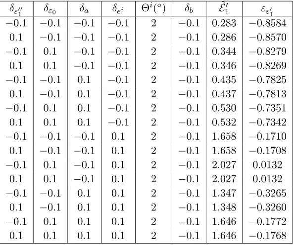
In Tables 3–4 we give the numerical values of ˜E1 and εε
1 in all of the 32 possible cases in which five
nuisance parameters areδ=±10% uncertain at a time.
Table 3. Retrieval of ε1 when five nuisance parameters (excepting Θi) areδ=±10% uncertain.
δε
1 δε0 δa δei Θ
i(◦) δ
b E˜1 εε1 −0.1 −0.1 −0.1 −0.1 2 −0.1 0.283 −0.8584
0.1 −0.1 −0.1 −0.1 2 −0.1 0.286 −0.8570
−0.1 0.1 −0.1 −0.1 2 −0.1 0.344 −0.8279 0.1 0.1 −0.1 −0.1 2 −0.1 0.346 −0.8269
−0.1 −0.1 0.1 −0.1 2 −0.1 0.435 −0.7825 0.1 −0.1 0.1 −0.1 2 −0.1 0.437 −0.7813
−0.1 0.1 0.1 −0.1 2 −0.1 0.530 −0.7351 0.1 0.1 0.1 −0.1 2 −0.1 0.532 −0.7342
−0.1 −0.1 −0.1 0.1 2 −0.1 1.658 −0.1710 0.1 −0.1 −0.1 0.1 2 −0.1 1.658 −0.1708
−0.1 0.1 −0.1 0.1 2 −0.1 2.027 0.0132 0.1 0.1 −0.1 0.1 2 −0.1 2.027 0.0132
−0.1 −0.1 0.1 0.1 2 −0.1 1.347 −0.3265 0.1 −0.1 0.1 0.1 2 −0.1 1.348 −0.3260
−0.1 0.1 0.1 0.1 2 −0.1 1.646 −0.1772 0.1 0.1 0.1 0.1 2 −0.1 1.646 −0.1768
Table 4. Retrieval of ε1 when five nuisance parameters (excepting Θi) areδ=±10% uncertain.
δε1 δε0 δa δei Θi(◦) δb E˜1 εε1 −0.1 −0.1 −0.1 −0.1 2 0.1 2.328 0.1638
0.1 −0.1 −0.1 −0.1 2 0.1 2.326 0.1632
−0.1 0.1 −0.1 −0.1 2 0.1 2.846 0.4321 0.1 0.1 −0.1 −0.1 2 0.1 2.845 0.4224
−0.1 −0.1 0.1 −0.1 2 0.1 1.658 −0.1710 0.1 −0.1 0.1 −0.1 2 0.1 1.658 −0.1708
−0.1 0.1 0.1 −0.1 2 0.1 2.027 0.0132 0.1 0.1 0.1 −0.1 2 0.1 2.027 0.0132
−0.1 −0.1 −0.1 0.1 2 0.1 ∞ ∞ 0.1 −0.1 −0.1 0.1 2 0.1 ∞ ∞
−0.1 0.1 −0.1 0.1 2 0.1 ∞ ∞ 0.1 0.1 −0.1 0.1 2 0.1 ∞ ∞
−0.1 −0.1 0.1 0.1 2 0.1 59.61 28.806 0.1 −0.1 0.1 0.1 2 0.1 59.59 28.794
These tables reveal that in sixteen of these cases,|εε1|>5|δ|, and in eight of these cases,|εε1| 5|δ|
(due to combined nuisance parameter uncertainty-induced instability).
It turns out that the pattern of retrieval error ofE1 is substantially the same as that ofE1.
6. CONCLUSION
Our inverse problem dealt with the retrieval of one of the seven parameters (either the real (ε1) or imaginary (ε1) part of the permittivity of a cylinder) that enter into a 2D quasistatic electricity configuration. The exact solution of the forward problem was obtained by separation of variables and employed to furnish the data serving as the input to the inverse problem. The retrieval model also relied on the separation of variables solution, but with one of the seven true parameters thereof replaced by a variable ε1 or ε1 and the remaining six (called nuisance) parameters by more or less well-known values. We solved the inverse problem: 1) by mathematically searching for the minimum of the cost functional K relative to continuous data on a measurement circle, and 2) by mathematically searching for the minimum of the cost functional K(N) relative to discrete data registered at N sensors on the measurement circle. This led to exact, mathematically-explicit solutions which lend themselves to a complete mathematical analysis of the manner in which the retrieval error varies as a function of the nuisance parameter uncertainties. In particular, we found that N = 3 sensors, equispaced over the angular range [0,2π[, are necessary and sufficient to provide the required data for the inversion. It was shown, in addition to the existence and uniqueness of the inverse problem solution satisfying pre-existing physical constraints, that this solution is unstable with respect to uncertainties concerning the nuisance parametersA,Ei andB, acting individually or in combination. These instabilities manifest themselves by extremely-large retrieval error in the neighborhoods of certain values of these nuisance parameters. It was also shown that, even quite far from these neighborhoods, the retrieval error|εε1|can be much larger
than a generic nuisance parameter uncertainty|δg|. Finally, it was found numerically, in agreement with
the theory, that the pattern of retrieval error of ε1 is much the same as that of ε1, notably as concerns the instability issue; moreover the relative retrieval error forM uncertain parameters turned out to be roughly proportional toM (outside of the instability regions, and for both the real and imaginary parts of the permittivity).
This investigation underlines the necessity, in parameter-retrieval inverse problems, to take account of nuisance parameter uncertainty in order to evaluate the accuracy of the retrieved parameter(s). In our study, only one parameter was retrieved at a time, while from one to five parameters were uncertain. It may be possible to reduce the global retrieval error by retrieving two or more parameters at a time while considering the remaining parameters to be uncertain, but this issue is out of the scope of the present study.
REFERENCES
1. Banks, H. T. and K. Kunisch, Estimation Techniques for Distributed Parameter Systems, Birkhauser, Boston, 1989.
2. Bauer N., K. Fajans, and S. Z. Lewin, “Refractometry,” Physical Methods of Organic Chemistry, A. Weissberger (ed.), Interscience, New York, 1960.
3. Bohren, C. F. and D. R. Huffman Absorption and Scattering of Light by Small Particles, Wiley, New York, 1983.
4. Chen, L., Z.-Y. Lei, R. Yang, X.-W. Shi, and J. Zhang, “Determining the effective electromagnetic parameters of bianisotropic metamaterials with periodic structures,”Progress In Electromagnetics Research M, Vol. 29, 79–93, 2013.
5. Chen, X., T. M. Grzegorczyk, B.-I. Wu, J. Pacheco Jr., and J. A. Kong, “Robust method to retrieve the constitutive effective parameters of metamaterials,” Phys. Rev. E, Vol. 70, 016608, 2004. 6. Chylek, P., V. Ramaswamy, A. Ashkin, and J. M. Dziedzic, “Simultaneous determination of
7. Emery, A. F., “The effect of correlations and uncertain parameters on the efficiency of estimating and the precision of estimated parameters,”Inverse Engineering Handbook, K. A. Woodbury (ed.), CRC Press, Boca Raton, 2003.
8. Hadamard, J. S., Lectures on Cauchy’s Problem in Linear Partial Differential Equations, Oxford University Press, Oxford, 1923.
9. Hasar, U. C., J. J. Barroso, C. Sabah, Y. Kaya, and M. Ertugrul, “Differential uncertainty analysis for evaluating the accuracy of S-parameter retrieval methods for electromagnetic properties of metamaterial slabs,” Opt. Express, Vol. 20, 29002–29022, 2012.
10. Hasar, U. C., J. J. Barroso, M. Ertugrul, C. Sabah, and B. Cavusoglu, “Application of a useful uncertainty analysis as a metric tool for assessing the performance of electromagnetic properties retrieval methods of bianisotropic metamaterials,”Progress In Electromagnetics Research, Vol. 128, 365–380, 2014.
11. Lefeuve-Mesgouez, G., A. Mesgouez, E. Ogam, T. Scotti, and A. Wirgin, “Retrieval of the physical properties of an anelastic solid half space from seismic data,” J. Appl. Geophys., Vol. 88, 70–82, 2013.
12. Morse, P. M. and H. Feshbach, Methods of Theoretical Phyics, Mc Graw-Hill, New York, 1953. 13. Neittaanmaki, P., M. Rudnicki, and A. Savini,Inverse Problems and Optimal Design in Electricity
and Magnetism, Clarendon Press, Oxford, 1996.
14. Pluchino, A. B., S. S. Goldberg, J. N. Dowling and C. M. Randall, “Refractive-index measurements of single micron-sized carbon particles,”Appl. Opt., Vol. 19, 3370–3372, 1980.
15. Sambuelli, L., “Uncertainty propagation using some common mixing rules for the modelling and interpretation of electromagnetic data,”Near Surf. Geophys., Vol. 7, 285–296, 2009.
16. Scotti, T. and A. Wirgin, “Multiparameter identification of a lossy fluid-like object from its transient acoustic response,”Inverse Prob. Sci. Engrg., Vol. 22, 1228–1258, 2014.
17. Seitz, F., The Modern Theory of Solids, Dover, New York, 1987.
18. Smith, D. R., D. C. Vier, T. Koschny, and C. M. Soukoulis, “Electromagnetic parameter retrieval from inhomogeneous metamaterials,” Phys. Rev. E, Vol. 71, 036617, 2005.
19. Von Hippel, A. R., Dielectrics and Waves, Chapman & Hall, London, 1954.
20. Vuye, G. and T. Lopez-Rios, “Precision in the ellipsometric determination of the optical constants of very thin films,”Appl. Opt., Vol. 21, 2968–2971, 1982.
21. Yilmaz, T., R. Foster, and Y. Hao, “Detecting vital signs with wearable wireless sensors,”Sensors, Vol. 10, 10837–10862, 2010.