Bootstrap Based Sequential Detection in Non-Gaussian
Correlated Clutter
Toufik Boukaba1, *, Mohammed Nabil El Korso2, Abdelhak M. Zoubir3, and Daoud Berkani4
Abstract—In this paper, sequential parametric detection problem is addressed for non-Gaussian correlated clutter. It is well known that the assumption of normally distributed clutter leads, mostly, to analytical expressions of the threshold as well the distribution of detection statistic. Nevertheless, due to the resolution improvement of recent sensing instruments such as high resolution radar, the Gaussian assumption is unrealistic since the clutter is nonhomogeneous. As a consequence, using non-Gaussian assumption of the clutter prevents, mostly, of obtaining analytical expressions of the threshold and the distribution of detection statistics. In this work, we overcome this issue by use of the so-called bootstrap techniques for dependent data. Numerical simulations reveal that our proposed method outperforms the classical and sequential non-bootstrap based detection schemes in terms of probability of detection and selects the optimum sample size needed to achieve the required detection performances.
1. INTRODUCTION
Detection step is one of the major tasks of radar systems. It refers to the decision made by a radar receiver regarding the presence or absence of an object of interest, namely the target, based on the received echo signal. This decision is then used to estimate parameters of the target such as location, velocity or shape.
Specifically, there are two kinds of radar echoes: i) useful signal, which is the echo signal reflected from the targets, such as aircrafts, ships, missiles, etc. and ii) clutter, which represents echo reflected from unrelated bodies such as land, sea surface, clouds, and rain. Detection of targets in clutter has been a constantly evolving field of study. In this context, the main challenge is to study the complex statistical properties of the clutter and to derive solutions to achieve optimal performances.
Among characteristics that describe statistical properties of the clutter, its distribution is of importance [1]. Formerly, the Gaussian assumption is the most well known and widely used distribution in many fields such as engineering and statistics [2]. Nowadays, in radar applications, it turns out to be not appropriate to model observed clutter especially in consideration of recent technological advances and resolution increase [3–5].
Starting from this evidence, many efforts have been emphasized on the study of non-Gaussian clutter in order to work out a model which can be applied to analysis and synthesis purposes [6–8]. A general agreement has been reached about the validity of the general and elegant impulsive model called compound-Gaussian. In this case, the baseband equivalent of clutter returns is modelled as the product of two mutually independent quantities: a complex, zero-mean, possibly correlated Gaussian process, also referred to as speckle, times the square root of a non-negative random scalar, referred to
Received 16 November 2017, Accepted 7 February 2018, Scheduled 13 February 2018 * Corresponding author: Toufik Boukaba ([email protected]).
as texture [9–11]. The clutter vector is then fully characterized by the unknown texture distribution and the speckle’s covariance matrix.
Based on this model, sub-optimal solutions have been derived following a generalized likelihood ratio test (GLRT) approach [12–14]. In practice, adaptive techniques are used to estimate unknown and space-time varying clutter parameters, using secondary signal-free data taken from range cells, surrounding the cell under test (CUT) and assumed to share the same statistical properties with the former.
In all developed methods, it is clearly stated that one of the major challenging difficulties is to estimate the covariance matrix of the speckle [15–17]. To perform this, one can appeals to non-parametric methods, where no assumption is made on clutter. In this case, the number of used secondary cells must be at least equal to the sample size. In non-stationary scenarios, this condition can be relaxed by using parametric methods, where the clutter is assumed to belong to a certain model.
Notwithstanding used approach, the global estimation-detection solution is generally based on a fixed sample size without any real-time adaptation. A beforehand performance analysis is used to select a rough size value, which is not necessarily the optimum regarding to the non-stationary character of the clutter and to computation costs.
In spite of their ability to minimize the required sample size to achieve given performance, the literature on sequential methods for radar detection is very scarce, particularly in the case of non-Gaussian clutter. In this paper, we use a sequential approach to reduce the sample size in the case of non-Gaussian correlated clutter. A parametric version of the adaptive normalized matched filter (ANMF) is used, where the clutter is approximated by an autoregressif (AR) process. A bootstrap procedure is then proposed to update detection thresholds.
The remainder of the paper is organized as follows: Section 2 is dedicated to the model setup and general background about sequential tests and bootstrap technique. Section 3 is devoted to the proposed approach, while Section 4 presents some results obtained using real data sets. Finally, Section 5 concludes the study.
2. MODEL SETUP AND THEORITICAL BACKGROUND
2.1. Model Setup
In radar detection problems, random signal received after the transmission ofN pulses is used to decide between two possible statistical hypotheses H0 and H1. These hypotheses correspond, respectively, to
the absence and the presence of a target. This can be described as:
H0:x=c H1:x=δd+c
(1)
where x= [x(0), x(1), . . . , x(N −1)]T is the received signal in the CUT,c= [c(0), c(1), . . . , c(N −1)]T the clutter vector, δ an unknown target’s deterministic amplitude, and d= [d(0), d(1), . . . , d(N −1)]T the target steering vector, with components dependent on fd, which is the assumed known Doppler frequency normalized with respect to the radar pulse repetition frequency (PRF).
The hypothesis test problem in Eq. (1) is solved by comparing a statistic Λ(x) computed from available data to a given threshold γ.
The parametric adaptive normalized matched filter, based on AR model (AR-PANMF) derived in [18] is used in this work. A set of secondary data, taken fromL range cells adjacent to the CUT, is used to estimate clutter unknown parameters.
The main assumption to be considered is that the clutter vector, in each secondary cell, is a zero mean compound Gaussian process approximated by an AR(p) process of assumed known orderp, driven by a white noise process [19, 20]. In summary, the AR-PANMF detector is given by:
ΛAR−PANMF(x) =
dHAHAx 2
dHAHAdx HAHAx
whereA is a lower triangularN×N matrix constructed with the estimated AR coefficients and is given by: A= ⎡ ⎢ ⎢ ⎢ ⎢ ⎢ ⎢ ⎢ ⎢ ⎣
1 0 . . . . . 0 ˆ
a1 1 0 . . . . .
. . . 0 . . . .
ˆ
ap . ˆa1 1 0 . . .
0 . . . . 0 . .
0 . . . . 0 .
. 0 . . . . 0
0 . 0 ˆap . ˆa1 1 ⎤ ⎥ ⎥ ⎥ ⎥ ⎥ ⎥ ⎥ ⎥ ⎦ (3)
where ˆa= [ˆa1,ˆa2, . . . ,ˆap]T is the vector of estimated AR coefficients obtained by minimizing the global forward prediction error for Lsecondary cells [18]:
ˆ
a=−
L
k=1
CHkCk
−1 L
k=1
CHk ck
(4)
in which,ck is the clutter vector in the k-th secondary cell, and Ck is given by:
Ck=
⎡ ⎢ ⎢ ⎢ ⎢ ⎢ ⎢ ⎢ ⎢ ⎢ ⎢ ⎣
0 0 . . . 0
ck(0) 0 . . . 0
ck(1) ck(0) . . . 0
..
. ... ... ...
ck(p−1) ck(p−2) . . . ck(0)
ck(p) ck(p−1) . . . ck(1) ..
. ... ... ...
ck(N −2) ck(N −3) . . . ck(N −p−1)
⎤ ⎥ ⎥ ⎥ ⎥ ⎥ ⎥ ⎥ ⎥ ⎥ ⎥ ⎦ (5)
Using the whitening effect of the matrix A, we obtain the following final expression:
ΛAR-PANMF(x) = ˆeHdˆex2
ˆ
eHdˆed ˆeHxeˆx
(6)
in which ˆex = Ax represents the forward prediction error sequence, while ˆed = Ad is the steering residuals vector.
2.2. Background on Sequential Detection
In the test defined by Eq. (1), two decisions are possible: accept or reject H0. This is exactly what is
done in the classical detection framework. In this case a fixed sample size and a single threshold are used. The threshold is fixed according to a given value of the first kind error, referred to as false alarm probability Pfa. In sequential tests, instead of the two obvious decisions, a third stage is introduced as
follows [21]:
(i) Accept the hypothesis H0.
(ii) Accept the hypothesis H1.
(iii) Consider an additional observation.
Two thresholds, AN (upper threshold) and BN (lower threshold), are then used and determined by
Pfa and the probability of miss detection Pm. These thresholds are used in order to ensure that the
required number of observations is minimized under the constraint that both Pfa and Pm are bounded
by pre-assigned valuesα and β:
Pfa = P(Λ(x)≥AN|H0)≤α (7) Pm = P(Λ(x)≤BN|H1)≤β (8)
• Decision 1 is made if Λ(x) is less than or equal to BN.
• Decision 2 is made if Λ(x) is greater than or equal to AN.
• Decision 3 is made if Λ(x) is inside the interval ]AN, BN[.
Precisely, any sequential test goes on as follows: based on the current observation, the test is terminated if the first or the second decision is made. Otherwise, an additional observation is considered and so on until a decision is made. Thresholds AN and BN are necessarily related to the distributions of the statistic Λ(x) respectively under H0 and under H1. An exact knowledge of these distributions is
then required to build a sequential test with performance set by bound values α and β. In practice, these distributions are seldom exactly known, and their parameters are space and time varying. In Section 3.2, we show how to come up with a sequential procedure based on thresholds update using bootstrap. Before that, we give a short overview about this technique.
2.3. Background on Bootstrap Technique
Nowadays, in most statistical signal processing applications, analytical results are pleasing and ensure the required rigour for parameters estimators. However, these solutions assume that the number of measurements, also called sample, is sufficiently large so that some assumptions are valid.
In many problems, these large sample methods are not usable. This is either due to processing time constraints or to the fact that the signal of interest is not stationary. In this case, analytical results cannot always be achieved and one may have to resort to Monte Carlo simulations. Unfortunately, this is not possible in practice because it requires the experiment to be repeated.
In this context, the bootstrap, which avoids the assumption of a large number of observations and does not need a new set of experiments, is an attractive solution [22].
Basically, the bootstrap is a computer-based method for assigning measures of accuracy to statistical estimates [22]. Meaning that, the bootstrap does with a computer what the experimenter would do in practice, if it were possible. Precisely simulate as much of the real world probability mechanism as possible, in which any unknowns are replaced with estimates from the observed data. The original observations are randomly rearranged, and reused to compute estimates. These reassignments and recomputations are done with a large number of times and treated as repeated experiments.
In the literature, diverse applications can be found in various fields [23–26]. Particularly, applications have been reported in radar and sonar signal processing [27–31].
In situations of unknown distributions and small samples, the bootstrap is highly appreciable as it substitutes estimates for unknowns and replaces mathematical analysis with computer simulations.
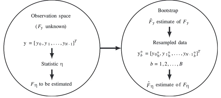
The basic principle of the bootstrap approach is summarized in Fig. 1.
Observation space
(Fy unknown)
y = [y0,y1, . . . ,yN 1]T
Statistic
F to be estimated
Bootstrap
ˆ
Fy estimate of Fy
Resampled data
yb = [y0 b, y1 b, . . . ,yN 1b]T
b = 1 , 2, . . . ,B
ˆ
F estimate o f F
Observation space
(Fy unknown)
y = [y0,y1, . . . ,yN -1]T
Statisticη
F to be estimated
Bootstrap
ˆ
Fy estimate of Fy
Resampled data
yb = [y0 b, y1 b, . . . ,yN - 1b]T
b = 1 , 2, . . . ,B
ˆ
F estimate o f F
η
*
η η
* * *
Assume that some statistic of interest η is calculated from a vector of random observations y= [y0, y1, . . . , yN−1]T, taken from an unknown distributionFy. In several applications, it is necessary to estimate the distributionFη of the statisticη. If the experiment is repeatable, one can use the Monte Carlo recurrence. Unfortunately, this is not always available in practice.
Bootstrap approach allows to do this without need to repeat the experiment. We first use the observation vectoryto obtain the estimate ofFy, denoted ˆFy. Then,Bbootstrap samples are generated from ˆFy. For each resample y∗, the statistic η∗ is calculated. At the end, the obtained B values of η are used to estimate Fη.
3. PROPOSED SEQUENTIAL DETECTION IN NON-GAUSSIAN CLUTTER
In the case of non-Gaussian clutter, it is convenient to consider that the distributions of the detection statistic belong to a given family, with unknown parameters. However, it is clear that any variation of these parameters will inevitably influence the performance of the detection scheme. In order to overcome this predictable performance degradation, it is appropriate to estimate these parameters and use theme to update thresholds.
In Section 3.1, we show that the distributions of ΛAR-PANMF, in non-Gaussian clutter, are of the
same type as those derived in [18], for Gaussian clutter. Recall that, in [18], performance evaluation has been handled under the assumption that these distributions where exactly the same. In Section 3.2, we use a bootstrap based method to estimate unknown parameters which characterize these distributions in non-Gaussian clutter and to update thresholds.
3.1. Analysis of the Distribution of the Parametric Detector AR-PANMF
Before the effective application of the bootstrap approach, recall that for Gaussian distributed clutter, the distribution of ΛAR-PANMFunderH0is a beta distribution, while it is a non-central beta distribution
underH1 [18]. These distributions are given respectively by:
F0Λ,N(λ) = Iλ(1, N −1) (9)
F1Λ,N(λ) =
+∞
j=0
1
j!
ξ
2
j
exp
−ξ
2
Iλ(1 +j, N −1) (10)
whereIx(b, c) is the regularized incomplete beta function ofx, with shape parametersband c;N is the sample size; ξ is the non-centrality parameter.
The main goal of this section is to explore how, for non-Gaussian clutter, empirical distributions of ΛAR-PANMFfit with generic models of the same type asF0Λ,N andF1Λ,N given by (9) and (10). This statistical analysis is performed using simulated data, within different clutter distributions and under shape parameters fluctuations.
For each clutter distribution, Monte Carlo runs are used to obtain a set of ΛAR-PANMF values.
Empirical cumulative distribution function (ECDF) is evaluated directly, while generic cumulative distribution function (CDF) is obtained using maximum likelihood (MLE) parameters estimation. Meaning that, for each vector of ΛAR-PANMF values, parameters of generic model are estimated using
MLE estimators. Theoretical CDF is then generated and compared to the ECDF. Besides, the Gaussian CDF, generated in the same way is considered as a benchmark.
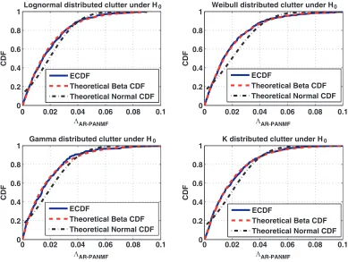
Four clutter distributions, consistent with the compound Gaussian model, are considered in this example. Namely lognormal, Weibull, gamma andkdistribution [11]. Under H0, and according to (9),
the beta CDF is considered as a generic model, whose parameters are estimated from ΛAR-PANMF
values. Precisely, the plots of Fig. 2 show the ECDF of the statistic ΛAR-PANMF for different clutter
distributions, under H0 compared to the generic Gaussian and beta CDF.
From these four graphs, it is clear that, under H0, the beta CDF provides a good fit to the
distribution of ΛAR-PANMF.
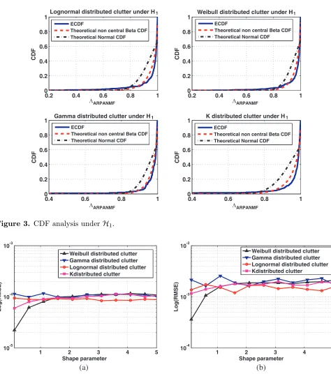
Under H1 and according to Eq. (10), the non-central beta CDF is considered as a generic model.
0 0.02 0.04 0.06 0.08 0.1 0
0.2 0.4 0.6 0.8
1Lognormal distributed clutter under H0
ΛAR-PANMF
CDF
0 0.02 0.04 0.06 0.08 0.1 0
0.2 0.4 0.6 0.8
1 Weibull distributed clutter under H0
ΛAR-PANMF
CDF
0 0.02 0.04 0.06 0.08 0.1 0
0.2 0.4 0.6 0.8
1 Gamma distributed clutter under H0
ΛAR-PANMF
CDF
0 0.02 0.04 0.06 0.08 0.1 0
0.2 0.4 0.6 0.8
1 K distributed clutter under H0
ΛAR-PANMF
CDF
ECDF
Theoretical Beta CDF Theoretical Normal CDF
ECDF
Theoretical Beta CDF Theoretical Normal CDF
ECDF
Theoretical Beta CDF Theoretical Normal CDF
ECDF
Theoretical Beta CDF Theoretical Normal CDF
Figure 2. CDF analysis underH0.
ξ. The plots of Fig. 3 show the ECDF of the statistic ΛAR-PANMF for different clutter distributions,
underH1 compared to generic Gaussian and non-central beta CDF. A good fitting between the ECDF
and the non-central beta model is noticed.
In real situations, many parameters can affect this goodness of fit. In the sequel, we measure it under fluctuations of: i) clutter distribution shape parameters, ii) signal-to-clutter ratio (SCR) under
H1and iii) Doppler shift underH0. We investigate the variations of the root mean square error (RMSE),
defined, between two functions F and G, as [33, 34]:
RMSE(F,G)=
1
Nx Nx
i=1
[F(xi)−G(xi)]2 (11)
where Nx is the size of the observation vector and xi the generic point of the X-axis in which both F
and G are evaluated.
Using the same simulation procedure as above, we consider the RMSE between generic CDF whose parameters are estimated using MLE and the ECDF. We evaluate this metric for different values of the shape parameter of each clutter model.
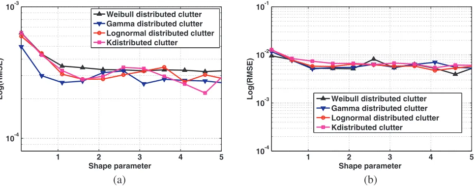
Under H0, the maximum value of the RMSE is recorded for the Doppler shift varying from −0.5
to 0.5. Under H1, the maximum value is recorded for SCR varying from −15 dB to 15 dB. Fig. 4 and
Fig. 5 show the variations of the RMSE respectively underH0 and underH1.
We note that, under parameters fluctuations, the RMSE exhibits better values for beta and non-central beta generic CDF, respectively underH0 and underH1.
3.2. Proposed Bootstrap Sequential-AR-PANMF (BS-AR-PANMF)
Based on the previous analysis, and instead of the challenging task, if feasable, which consists on deriving
0.2 0.4 0.6 0.8 1 0
0.2 0.4 0.6 0.8
1Lognormal distributed clutter under H1
ΛARPANMF
CDF
0.2 0.4 0.6 0.8 1 0
0.2 0.4 0.6 0.8
1 Weibull distributed clutter under H1
ΛARPANMF
CDF
0.4 0.6 0.8 1
0 0.2 0.4 0.6 0.8
1 Gamma distributed clutter under H1
ΛARPANMF
CDF
0.4 0.6 0.8 1
0 0.2 0.4 0.6 0.8
1 K distributed clutter under H1
ΛARPANMF
CDF
ECDF
Theoretical non central Beta CDF Theoretical Normal CDF
ECDF
Theoretical non central Beta CDF Theoretical Normal CDF
ECDF
Theoretical non central Beta CDF Theoretical Normal CDF
ECDF
Theoretical non central Beta CDF Theoretical Normal CDF
Figure 3. CDF analysis underH1.
1 2 3 4 5
10-5 10-4 10-3
Shape parameter
Log(RMSE)
Weibull distributed clutter Gamma distributed clutter Lognormal distributed clutter Kdistributed clutter
1 2 3 4 5
10-4 10-3 10-2
Shape parameter
Log(RMSE)
Weibull distributed clutter Gamma distributed clutter Lognormal distributed clutter Kdistributed clutter
(a) (b)
Figure 4. RMSE variations underH0: (a) Beta generic CDF, (b) Gaussian generic CDF.
approach. The analysis above suggests to assume F0Λ,N to be a beta distribution while F1Λ,N is assumed to be a non-central beta distribution, both with unknown parameters. A bootstrap method will be used to estimate these parameters.
In radar applications, the assumption of independent clutter samples breaks down [3]. Consequently, we propose in the sequel to use moving block bootstrap which is the appropriate method in this context [22, 35, 36].
1 2 3 4 5 10-4
10-3
Shape parameter
Log(RMSE)
Weibull distributed clutter Gamma distributed clutter Lognormal distributed clutter Kdistributed clutter
1 2 3 4 5
10-4 10-3 10-2 10-1
Shape parameter
Log(RMSE) Weibull distributed clutter Gamma distributed clutter Lognormal distributed clutter Kdistributed clutter
(a) (b)
Figure 5. RMSE variations underH1: (a) Non-central beta generic CDF, (b) Gaussian generic CDF.
resample is then formed by concatenating these blocks. Before detailing the proposed approach, let us recall that the expressions of the lower thresholdBN and the higher thresholdAN to be used are given, respectively by [18]:
NTr−p
k=1
NTr−p k
F1Λ,N(BN)k[1−F1Λ,N(BN)]NTr−p−k−β= 0 (12)
AN =F0Λ−1,N
(1−α)1/(NTr−p) (13)
where NTr is the truncated sample number, which is chosen to be sufficiently large (NTr p+ 1) to
guarantee that the probability that the stopping timeNstopis higher thanNTr is sufficiently small under
each hypothesis.
Based on the analysis given in 3.1, we assume that F0Λ,N is a beta distribution function with unknown shape parameters a0 and b0 and that F1Λ,N is a non-central beta distribution function also with unknown shape and non-centrality parameters a1,b1 and ξ1.
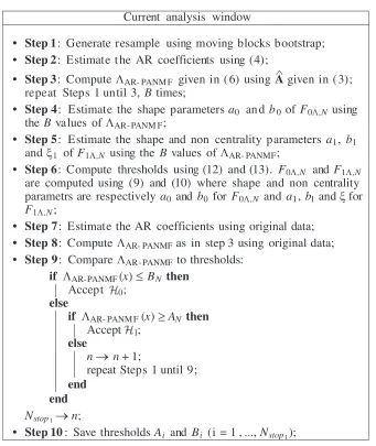
In the sequel, these unknown parameters are estimated using a moving block bootstrap procedure. They are then used to compute the thresholdsBN andAN which are used to perform a sequential test. In the sequel, we assume that the AR orderp is known and that, at the beginning of the process, an analysis window of (p+ 1) data, both in the CUT and in one secondary cell on each side of the CUT, is available. According to the general frame of sequential detection as described in Section 2.2, the proposed approach is performed in the following way:
• Using the first analysis window, the shape and non-centrality parameters of F0Λ,N and F1Λ,N are estimated using the vector of ΛAR-PANMF values obtained thanks to the moving block bootstrap.
ThresholdsAN and BN are then computed and memorized for all sample sizes until the decision is made. Assume that the decision is made for a sample size Nstop1.
• For the next analysis window, the memorized thresholds are used. If the decision is made for a sample size less than or equal to Nstop1 there is no need to use bootstrap function. If the decision
requires more samples, the shape and non-centrality parameters ofF0Λ,N and F1Λ,N are estimated in the same way as above. Thresholds are then updated and stored for sizesNstop1+ 1, . . . , Nstop2.
• For thei-th analysis window, the bootstrap function is used only if the decision requires more than
Nstopi−1 samples.
The overall procedure is summarized in Tab. 1 and Tab. 2.
Table 1. BS-AR-PANMF algorithm for the current analysis window.
Current analysis window
• Step 1: Generate resample using moving blocks bootstrap;
• Step 2: Estimate t he AR coefficients using (4);
• Step 3: Compute ΛAR- PANM F given in ( 6) using Agiven in ( 3);
repeat Steps 1 until 3, B times;
• Step 4: Estimate the shape parametersa0 an d b0 ofF0Λ,N using
the B values ofΛAR- PANM F;
• Step 5: Estimate the shape and non centrality parameters a1, b1
and ξ1 ofF1Λ,N using the B values ofΛAR- PANMF;
• Step 6: Compute thresholds using (12) and (13). F0Λ,N andF1Λ,N
are computed using (9) and (10) where shape and non centrality
parametrs are respectively a0 and b0 for F0Λ,N and a1, b1and ξ for
F1Λ,N;
• Step 7: Estimate the AR coefficients using original data;
• Step 8: ComputeΛAR- PANMFas in step 3 using original data;
• Step 9: Compare ΛAR- PANMF to thresholds:
if ΛAR- PANMF(x) BN then
Accept 0;
else
if ΛAR- PANM F(x) AN then
Accept 1;
else
n n+ 1;
repeat Steps 1 until 9; end
end
Nstop1 n;
• Step 10: Save thresholdsAi and Bi (i = 1 , ...,Nstop1);
≤
≥
→
→
∧
4. RESULTS
Performance of the proposed approach is evaluated in terms of detection probability (Pd) and the
required size to achieve it. A comparison of the two aspects is assessed between the proposed BS-AR-PANMF and the sequential approach, based on thresholds derived for Gaussian distributed clutter.
To carry out this, we use real sea clutter data sets collected by the X-band McMaster university, Canada, IPIX radar in February 1998.
After preprocessing, the data are stored in anNt×Nc matrix.
Three data files are used, which correspond to range resolutions 30, 15 and 03 meters and to respective polarities HH,HV and V V. A summary description of the used data files, given in [18], is reminded in Tab. 3.
In order to give a general outline about computational cost carried out by the proposed approach, we evaluate the number of bootstrap function uses for analysis the 60000×34 data sets. Tab. 4 and Tab. 5 provide obtained values respectively, under H0, for the Doppler shift varying from−0.5 to 0.5
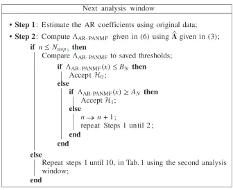
Table 2. BS-AR-PANMF algorithm for the next analysis window.
Next analysis window
• Step 1: Estimate the AR coefficients using original data;
• Step 2: ComputeΛAR- PANM F given in (6) using Agiven in (3);
if n Nstop1 then
Compare ΛAR - PANMF to saved thresholds;
if ΛAR- PANMF(x) BN then
Accept 0;
else
if ΛAR- PANMF(x) AN then
Accept 1;
else
n n + 1;
repeat Steps 1 until 2 ; end
end else
Repeat steps 1 until 10, in Tab. 1 using the second analysis window;
end
≤
≤
≥
→
∧
Table 3. Characteristics of the used real data files.
File 1 File 2 File 3
File name 19980223 165836 19980223 171533 19980223 170435 Date February 23 1998 February 23 1998 February 23 1998 Time 16 : 58 : 36 17 : 15 : 33 17 : 04 : 35
RF Fr´equency (GHz) 9.39 9.39 9.39
Pulse width (ns) 200 20 100
PRF (Hz) 1000 1000 1000
Range resolution (m) 30 03 15
Polarization Agility Agility Agility Azimuth angle (◦) 343.059 344.05 344.517
Grazing angle (◦) 0.32 0.32 0.32
Range (m) 3989 3600 3996
Radar height (m) 20 20 20
Radar latitude (◦) 43.21 43.21 43.21 Radar longitude (◦) 79.60 79.60 79.60 Number of pulsesNt 60000 60000 60000
Number of cellsNc 34 34 34
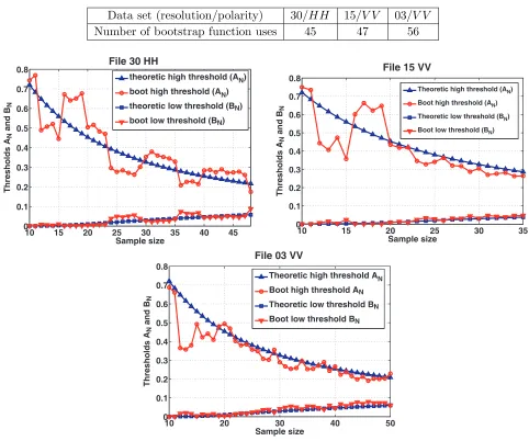
4.1. Thresholds Variations
Table 4. Number of bootstrap function uses for analysis of all the 60000×34 data sets under H0, for
the Doppler shift varying from−0.5 to 0.5.
Data set (resolution/polarity) 30/HH 15/V V 03/V V
Number of bootstrap function uses 39 40 47
Table 5. Number of bootstrap function uses for analysis of all the 60000×34 data sets under H1, for
SCR ranging from−15 dB to 15 dB.
Data set (resolution/polarity) 30/HH 15/V V 03/V V
Number of bootstrap function uses 45 47 56
10 15 20 25 30 35 40 45
0 0.1 0.2 0.3 0.4 0.5 0.6 0.7 0.8
Sample size
Thresholds A
N
and B
N
File 30 HH
theoretic high threshold (AN)
boot high threshold (AN)
theoretic low threshold (BN)
boot low threshold (BN)
10 15 20 25 30 35
0 0.1 0.2 0.3 0.4 0.5 0.6 0.7 0.8
Sample size
Thresholds A
N
and B
N
File 15 VV
Theoretic high threshold (AN)
Boot high threshold (AN)
Theoretic low threshold (BN)
Boot low threshold (BN)
10 20 30 40 50
0 0.1 0.2 0.3 0.4 0.5 0.6 0.7 0.8
Sample size
Thresholds A
N
and B
N
File 03 VV
Theoretic high threshold AN
Boot high threshold AN
Theoretic low threshold BN
Boot low threshold BN
Figure 6. ThresholdsAN and BN obtained using bootstrap (files 30HH, 15V V and 03V V).
Figure 6 represents the obtained thresholds. In each sub-figure, we also show, as a benchmark, the thresholds obtained for the Gaussian case, where shape parameters of F0Λ,N and F1Λ,N are 1 and
N −1 [18].
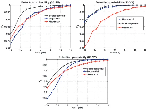
4.2. Performance under H1
Figure 7 represents the probabilities of detection obtained using bootstrap estimation of shape parameters, compared to ones obtained using the sequential approach based on theoretic thresholds which correspond to the Gaussian case and the ones obtained using the classical fixed size method. For the 30/HHand 15/V V data sets, the probability of detection is slightly improved. For the 03/V V data set the improvement is about 13%. Fig. 8 shows the size ratios Nf/Ns obtained using the sequential
-15 -10 -5 0 5 10 15
0.97 0.975 0.98 0.985 0.99 0.995 1
SCR (dB)
Pd
Detection probability (30 HH)
Bootsequential Sequential Fixed size
-15 -10 -5 0 5 10 15
0.94 0.95 0.96 0.97 0.98 0.99 1
SCR (dB)
Pd
Detection probability (15 VV)
Sequential
Bootsequential
fixed size
-15 -10 -5 0 5 10 15
0.65 0.7 0.75 0.8 0.85 0.9 0.95 1
SCR (dB)
Pd
Detection probability (03 VV)
Bootsequential Sequential Fixed size
Figure 7. Probability of detection obtained using bootstrap (files 30HH, 15V V and 03V V).
-152 -10 -5 0 5 10 15
2.5 3 3.5 4 4.5 5 5.5 6
SCR (dB)
Nf
/ N
s
Size ratio under H1 (30 HH)
Bootsequential Sequential
-152 -10 -5 0 5 10 15
3 4 5 6 7 8
SCR (dB)
Nf
/ N
s
Size ratio under H1 (15 VV)
Bootsequential
-152 -10 -5 0 5 10 15 2.5
3 3.5 4 4.5 5 5.5
SCR (dB)
Nf
/ N
s
Size ratio under H1 (03 VV)
Bootsequential Sequential
Figure 8. Size ratio, underH1, obtained using bootstrap (files 30HH, 15V V and 03V V).
-0.5 -0.4 -0.3 -0.2 -0.12 0 0.1 0.2 0.3 0.4 0.5
2.2 2.4 2.6 2.8 3 3.2
fd Nf
/ N
s
Size ratio under H0 (30 HH)
Sequential Bootsequential
-0.5 -0.4 -0.3 -0.2 -0.1 00000000000 0.1 0.2 0.3 0.4 0.5 2.2
2.4 2.6 2.8 3 3.2 3.4
fd
Nf
/ N
s
Size ratio under H0 (15 VV)
Sequential Bootsequential
-0.5 -0.4 -0.3 -0.2 -0.1 0 0.1 0.2 0.3 0.4 0.5 2.1
2.2 2.3 2.4 2.5 2.6 2.7 2.8 2.9 3 3.1
fd Nf
/ N
s
Size ratio under H0 (03 VV)
Sequential Bootsequential
Figure 9. Size ratio, underH0, obtained using bootstrap (files 30HH, 15V V and 03V V).
An intuitive reason for this high relative improvement for the 03/V V data set is the fact that as the resolution increases, the clutter distribution is farther from the Gaussian model.
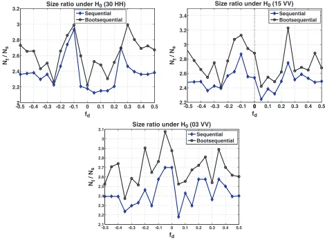
4.3. Performance under H0
Under H0, the probability of false alarm Pfa has the same behaviour as in [18]. The results presented
here concern the gain brought by the proposed BS-AR-PANMF in terms of sample size.
Figure 9 shows the size ratios obtained using the sequential approach and the BS-AR-PANMF. As underH1, we note that the higher is the resolution, the better is the sample size gain.
5. CONCLUSIONS
In this paper, we have proposed a new approach to apply the parametric bootstrap in sequential detection for composite hypothesis testing in non-Gaussian clutter. The detection statistic is based on the approximation of the clutter as an AR process.
Simulation study has shown that the distributions of this parametric detector, under underH0 and
under H1 fit well, respectively, the beta and the non-central beta models, with unknown parameters.
The moving block bootstrap is then used to estimate these parameters and to update the thresholds in an adaptive manner based on current observations. The general computation cost is reduced by saving updated thresholds and using theme as long as they allow to make a decision until given sample sizes. Detection performance and required sample sizes are investigated using real data. For all used data files, the proposed BS-AR-PANMF provides detection performance better than that of the sequential AR-PANMF detector based on analytic thresholds derived for Gaussian clutter. In terms of required sample sizes, the BS-AR-PANMF gives acceptable gains.
Under the two hypothesis and regarding detection probabilities and required sample sizes, the performance is better for high resolution. This is because in this case the distribution of the clutter is far from the Gaussian assumption, and thresholds update is more suitable.
ACKNOWLEDGMENT
The authors would like to thank Prof. Fulvio GINI from Pisa University, Italy, for kindly providing the Ipix data sets.
REFERENCES
1. Watts, S., “Radar clutter and multipath propagation,” IEE Proceedings F (Radar and Signal Processing), Vol. 138, 73–74, IET, 1991.
2. Park, S., E. Serpedin, and K. Qaraqe, “Gaussian assumption: The least favorable but the most useful,” IEEE Signal Processing Magazine, Vol. 30, No. 3, 183–186, 2013.
3. Greco, M., F. Gini, and M. Rangaswamy, “Statistical analysis of measured polarimetric clutter data at different range resolutions,”Proceedings of the IEE, Radar Sonar and Navigation, Vol. 153, No. 6, 473–481, 2006.
4. Conte, E., A. De Maio, and C. Galdi, “Statistical analysis of real clutter at different range resolutions,” IEEE Transactions on Aerospace and Electronic Systems, Vol. 40, No. 3, 903–918, 2004.
5. Carretero-Moya, J., J. Gismero-Menoyo, ´A. Blanco-del Campo, and A. Asensio-Lopez, “Statistical analysis of a high-resolution sea-clutter database,” IEEE Transactions on Geoscience and Remote Sensing, Vol. 48, No. 4, 2024–2037, 2010.
6. Ward, K. D., S. Watts, and R. J. Tough, Sea Clutter: Scattering, the K Distribution and Radar Performance, Vol. 20, IET, 2006.
8. Gini, F., “A cumulant-based adaptive technique for coherent radar detection in a mixture of kdistributed clutter and gaussian disturbance,”IEEE Transactions on Signal Processing, Vol. 45, No. 6, 1997, 1507–1519.
9. Ward, K., “Compound representation of high resolution sea clutter,” Electronics Letters, Vol. 17, No. 16, 561–563, 1981.
10. Lampropoulos, G., A. Drosopoulos, N. Rey, et al., “High resolution radar clutter statistics,” IEEE Transactions on Aerospace and Electronic Systems, Vol. 35, No. 1, 43–60, 1999.
11. Rangaswamy, M., D. D. Weiner, and A. Ozturk, “Non-gaussian random vector identification using spherically invariant random processes,”IEEE Transactions on Aerospace and Electronic Systems, Vol. 29, No. 1, 1993, 111–124.
12. Conte, E., M. Lops, and G. Ricci, “Asymptotically optimum radar detection in compound-gaussian clutter,”IEEE Transactions on Aerospace and Electronic Systems, Vol. 31, No. 2, 617–625, 1995. 13. Gini, F. and M. Greco, “Suboptimum approach to adaptive coherent radar detection in
compound-Gaussian clutter,”IEEE Transactions on Aerospace and Electronic Systems, Vol. 35, No. 3, 1095– 1104, 1999.
14. Sangston, K. J., F. Gini, M. V. Greco, and A. Farina, “Structures for radar detection in compound gaussian clutter,”IEEE Transactions on Aerospace and Electronic Systems, Vol. 35, No. 2, 445–458, 1999.
15. Conte, E., A. De Maio, and G. Ricci, “Recursive estimation of the covariance matrix of a compound-Gaussian process and its application to adaptive CFAR detection,” IEEE Transactions on Signal Processing, Vol. 50, No. 8, 1908–1915, 2002.
16. Gini, F. and M. Greco, “Covariance matrix estimation for cfar detection in correlated heavy tailed clutter,”Signal Processing, Vol. 82, No. 12, 1847–1859, 2002.
17. Pascal, F., P. Forster, J.-P. Ovarlez, and P. Larzabal, “Performance analysis of covariance matrix estimates in impulsive noise,IEEE Transactions on Signal Processing, Vol. 56, No. 6, 2008, 2206– 2217.
18. Boukaba, T., A. M. Zoubir, and D. Berkani, “Parametric detection in non-stationary correlated clutter using a sequential approach,” Digital Signal Processing, Vol. 36, 2015, 69–81.
19. Ramakrishnan, D. and J. Krolik, “Adaptive radar detection in doubly nonstationary autoregressive doppler spread clutter,” IEEE Transactions on Aerospace and Electronic Systems, Vol. 45, No. 2, 484–501, 2009.
20. Dong, Y., “Parametric adaptive matched filter and its modified version,” Defense Science and Technology Organization South Australia, 2006.
21. Wald, A., Sequential Analysis, Courier Dover Publications, 1947.
22. Zoubir, A. M. and D. R. Iskander, Bootstrap Techniques for Signal Processing, Cambridge University Press, 2004.
23. Chernick, M. R.,Bootstrap Methods: A Practitioner’s Guide, Wiley-Interscience, 1999.
24. Chernick, M. R., W. Gonz´alez-Manteiga, R. M. Crujeiras, and E. B. Barrios, “Bootstrap methods,”
International Encyclopedia of Statistical Science, 169–174, Springer, 2011.
25. Zoubir, A. M. and D. R. Iskandler, “Bootstrap methods and applications,”IEEE Signal Processing Magazine, Vol. 24, No. 4, 10–19, 2007.
26. Suratman, F. Y. and A. M. Zoubir, “Bootstrap based sequential probability ratio tests,” IEEE International Conference on Acoustics, Speech and Signal Processing (ICASSP), 6352–6356, IEEE, 2013.
27. Nagaoka, S. and O. Amai, “A method for establishing a separation in air traffic control using a radar estimation accuracy of close approach probability,”J. Japan Ins. Navigation, Vol. 82, 53–60, 1990.
29. Krolik, J., G. Niezgoda, and D. Swingler, “A bootstrap approach for evaluating source localization performance on real sensor array data,” IEEE International Conference on Acoustics, Speech and Signal Processing (ICASSP), 1281–1284, IEEE, 1991.
30. B¨ohme, J. and D. Maiwald, “Multiple wideband signal detection and tracking from towed array data,” IFAC Proceedings, Vol. 27, No. 8, 107–112, 1994.
31. Debes, C., C. Weiss, A. M. Zoubir, and M. G. Amin, “Distributed target detection in through-the-wall radar imaging using the bootstrap,”IEEE International Conference on Acoustics Speech and Signal Processing (ICASSP), 3530–3533, IEEE, 2010.
32. Walck, C., “Hand book on statistical distributions for experimentalists,” Tech. Rep., Particle Physics Group, University of Stockholm, 1996.
33. Basseville, M., “Distance measures for signal processing and pattern recognition,” Signal Processing, Vol. 18, No. 4, 349–369, 1989.
34. Martinez, W. L. and A. R. Martinez, Computational Statistics Handbook with MATLAB, Vol. 22, CRC Press, 2007.
35. Davison, A. C. and D. V. Hinkley, Bootstrap Methods and Their Application, Vol. 1, Cambridge University Press, 1997.