Pre-attentive segmentation in the
primary visual cortex
Zhaoping Li
Gatsby Computational Neuroscience Unit University College London
17 Queen Square, London, WC1N, 3AR, U.K. email: [email protected]
fax: 44 171 391 1173
Short title: Pre-attentive segmentation in V1.
Published inSpatial Vision, Volumn 13(1), p. 25-50, (2000).
Abstract
1 Introduction
In early stages of visual processing, individual neurons respond directly only to stimuli in their classical receptive fields (CRFs)(Hubel and Wiesel, 1962). These CRFs sample thelocal contrast information in the input but are too small to cover visual objects at a
globalscale. Recent experiments show that the responses of primary cortical (V1) cells are significantly influenced by stimuli nearby and beyond their CRFs (Allman et al 1985, Knierim and Van Essen 1992, Gilbert, 1992, Kapadia et al 1995, Sillito et al 1995, Lamme, 1995, Zipser et al 1996, Levitt and Lund 1997). These contextual influences are in general suppressive and depend on the relative orientations of the stimuli within and beyond the CRF (Allman et al, 1985, Knierim and Van Essen 1992, Sillito et al 1995, Levitt and Lund 1997). In particular, the response to an optimal bar in the CRF is suppressed significantly by similarly oriented bars in the surround — iso-orientation suppression (Knierim and Van Essen 1992). The suppression is reduced when the orientations of the surround bars are random or different from the bar in the CRF (Knierim and Van Essen 1992, Sillito et al 1995). However, if the surround bars are aligned with the optimal bar inside the CRF to form a smooth contour, then suppression becomes facilitation (Kapa-dia et al 1995). The contextual influences are apparent within 10-20 ms after the cell’s initial response (Knierim and Van Essen 1992, Kapadia et al 1995), suggesting that mech-anisms within V1 itself are responsible (see discussion later on the different time scales observed by Zipser et al 1996). Horizontal intra-cortical connections linking cells with non-overlapping CRFs and similar orientation preferences have been observed and hy-pothesized to be the neural substrate underlying these contextual influences (Gilbert and Wiesel, 1983, Rockland and Lund 1983, Gilbert, 1992). There have also been the-oretical studies of the mechanisms and phenomena of the contextual influences (e.g., Somers et al 1995, Stemmler et al 1995). However, insights into the computational roles of contextual influences have been limited to mainly contour or feature linking (Allman et al 1995, Gilbert, 1992, see more references in Li 1998a).
regions or targets do not pop out pre-attentively.
2 The principle and its implementation
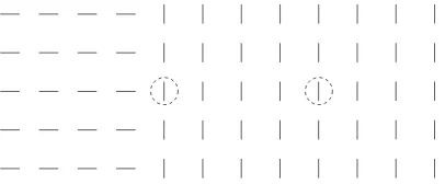
Figure 1: An input image, and two examples of CRFs marked by two dashed circles, which have the same stimulus within the CRFs but different contextual surrounds. A cell tuned to vertical orientation experiences less iso-orientation suppression in the left CRF than the right one.
tex-A Visual space and edge detectors
A Sampling location One of the edge/bar
this sampling location. detectors (pairs) at
B Neural connection pattern. Solid: , Dashed:
C Model Neural Elements and functions —
a schematic simplified for cells tuned to horizontal orientation only
!! !! !! !! "" "" "" "" ## ## ## ## $$ $$ $$ $$ %% %% %% %% && && && && '' '' '' '' (( (( (( (( )) )) )) )) ** ** ** ** ++ ++ ++ ++ ,, ,, ,, ,, --.. .. .. .. // // // // 00 00 00 00 11 11 11 11 22 22 22 22 33 33 33 33 44 44 44 44 55 55 55 55 66 66 66 66 77 77 77 77 88 88 88 88 99 99 99 99 :: :: :: :: ;; ;; ;; ;; << << << << == == == == >> >> >> >> ?? ?? ?? ?? @@ @@ @@ @@ AA AA AA AA BB BB BB BB CC CC CC CC DD DD DD DD EE EE EE EE FF FF FF FF GG GG GG GG HH HH HH HH II II II II JJ JJ JJ JJ KK KK KK KK LL LL LL LL MM MM MM MM NN NN NN NN OO OO OO OO PP PP PP PP QQ QQ QQ QQ RR RR RR RR SS SS SS SS TT TT TT TT UU UU UU UU VV VV VV VV WW WW WW WW XX XX XX XX YY YY YY YY ZZ ZZ ZZ ZZ [[ [[ [[ [[ \\ \\ \\ \\
(filtered through the CRFs)
responses connection inter-pairing 1:1 neurons
(After intracortical interactions)
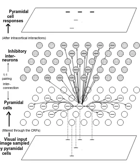
Inhibitory inter-Pyramidal cells Visual input image sampled by pyramidal cells Pyramidal cell Figure 2:
ture boundaries or segments of a contour than inside homogeneous regions (Nothdurft, 1994, Gallant et al 1995, Kapadia et al 1995).
lu-Figure 2: (Caption for figure in previous page)A:Visual inputs are sampled in a discrete grid by edge/bar detectors, modeling CRFs for V1 layer 2-3 cells. Each grid point has 12 neuron pairs (seeC), one per bar segment. All 12 pairs or 24 cells at a grid point share the same CRF center, but are tuned to different ori-entations spanning , thus modeling a hypercolumn. A bar segment in one hypercolumn can interact with another in a different hypercolumn via monosy-naptic excitation or disymonosy-naptic inhibition (seeB, C).B: A schematic of the horizontal connection pattern from the center (thick solid) bar to neighboring bars within a finite distance (a few CRF sizes). ’s contacts are shown by thin solid bars. ’s are shown by thin dashed bars. Each CRF has the same con-nection pattern, suitably translated and rotated from this one. C:The neural elements and connections for cells tuned to horizontal orientations only (to avoid excessive clutter in the figure), and an illustration of the function of this system. Only connections to and from the central pyramidal cell are drawn. A horizontal bar, marking the preferred stimulus of the cell, is drawn on the cen-tral pyramidal cell and all other pyramidal or interneurons that are linked to it by horizontal connections. The central pyramidal sends axons (monosynap-tic connections ) to other pyramidals that are displaced from it locally and roughly horizontally, and to the interneurons displaced locally and roughly vertically in the input image plane. The bottom plate depicts an example of in-put image containing 5 horizontal bars of equal contrast, each gives inin-put to a pyramidal cell with the corresponding CRF (the correspondences are indicated by the dashed lines). These 5 pyramidal cells give higher response levels to the 3 bars aligned horizontally but lower responses to the 2 bars displaced vertical from them, as illustrated in the top plate. This is because the 3 horizontally aligned bars facilitate each other via the monosynaptic connections , while the vertically displaced bars inhibit each other disynaptically via .
minance, or stereo. Since it focuses on the role of contextual influences in segmentation, the model includes mainly layer 2-3 orientation selective cells and ignores the mech-anism by which their CRFs are generated. Inputs to the model are images filtered by the edge- or bar-like local CRFs of V1 cells (we use ‘edge’ and ‘bar’ interchangeably). To avoid confusion, this paper uses the term ‘edge’ only for local luminance contrast, a boundary of a region is termed ‘boundary’ or ‘border’ which may or may not (especially for texture regions) correspond to any actual ‘edges’ in the image. Cells are connected by horizontal intra-cortical connections (Rockland and Lund 1983, Gilbert and Wiesel, 1983, Gilbert, 1992). These transform patterns of direct, CRF, inputs to the cells into patterns of contextually modulated output firing rates of the cells.
Fig. 2 shows the elements of the model and the way they interact. At each sampling location there is a model V1 hypercolumn composed of cells whose CRFs are centered at and that are tuned to different orientations spanning (Fig. 2A). Based on experimental data (White, 1989, Douglas and Martin 1990), for each angle at location
real cortex, thus a 1:1 ratio between the numbers of pyramidal cells and interneurons in the model does not imply such a ratio in the cortex. For convenience, we refer to the cells tuned to at location as simply the edge or bar segment .
Visual inputs are mainly received by the pyramidal cells, and their output activities (which are sent to higher visual areas) quantify the saliencies of their associated edge segments. The inhibitory cells are treated as interneurons. The input
to pyrami-dal cell is obtained by filtering the input image through the CRF associated with . Hence, when the input image contains a bar of contrast
at location and oriented at angle , pyramidal cells are excited if is equal or close to . The value
will be
where
! #"#$ describes the orientation tuning curve of the cell.
Fig. 2C shows an example in the case that the input image contains just horizontal bars. Only cells preferring orientations close to horizontal in locations receiving visual input are directly excited — cells preferring other orientations or other locations are not directly excited. In this example, the five horizontal bars have the same input strengths, and so the input
to the five corresponding pyramidal cells are of the same strengths as well. We omit cells whose preferred orientations are not horizontal but within the tuning width from horizontal for the simplicity of this argument.
In the absence of long-range intra-cortical interactions, the reciprocal connections between the pyramidal cells and their partner inhibitory interneurons would merely provide a form of gain control mechanism on input
. The response from the pyrami-dal cell would only be a function of its direct input
. This would make the spatial pattern of pyramidal responses from V1 simply proportional to the spatial pattern of
up to a context-independent (ielocal), non-linear, contrast gain control. However, in fact, the responses of the pyramidal cells are modified by the activities of nearby pyra-midal cells via horizontal connections. The influence is excitatory via monosynaptic connections and inhibitory via disynaptic connections through interneurons. The in-teractions make a cell’s response dependent on inputs outside its CRF, and the spatial pattern of response ceases being proportional to the input pattern
. Fig. 2B,C show the structure of the horizontal connections. Connection%
&'#)( from pyramidal cell*+ to pyramidal cell mediates monosynaptic excitation. Connection
%
&'#)(-,
if these two segments are tuned to similar orientations/. + and the centers and* of their CRFs are displaced from each other along their preferred orientation10 +. Connection2
&'33(
from pyramidal cell*+ to the inhibitory interneuron mediates disynaptic inhibition from the pyramidal cell* + to the pyramidal cell . Connection
2
&'33(4,
if the preferred orientations of the two cells are similar5.
+, but the centers and* of their CRFs are displaced from each other along a direction orthogonal to their preferred orientations. The reasons for the different designs of the connection patterns of J and W will be clear later.
In Fig. 2C, cells tuned to non-horizontal orientations are omitted to illustrate the in-tracortical connections without excessive clutter in the figure. Here, the monosynaptic connections% link neighboring horizontal bars displaced from each other roughly hor-izontally, and the disynaptic connections2 link those bars displaced from each other more or less vertically in the visual input image plane. The full horizontal connection structure from a horizontal bar to bar segments including the non-horizontal ones is shown in Fig. 2B. Note that all bars in Fig. 2B are near horizontal and are within a distance of a few CRFs. The connection structure resembles a bow-tie, and is the same for every pyramidal cell within its ego-centric frame.
differ-ent output activities in response to input bars of equal contrast. The three horizon-tally aligned bars in the input induce higher output responses because they facilitate each other’s activities via the monosynaptic connections %
&'#)(
. The other two hori-zontal bars induce lower responses because they receive no monosynaptic excitation from others and receive disynaptic inhibition from the neighboring horizontal bars that are displaced vertically (and are thus not co-aligned with them). Note that the three horizontally aligned bars, especially the middle one, also receive disynaptic inhibitions from the two vertically displaced bars.
In the case that the input is a homogeneous texture of horizontal bars, each bar will receive monosynaptic excitation from its (roughly) left and right neighbors but disynaptic inhibition from its (roughly) top and bottom neighbors. Our intra-cortical connections are designed so that the sum of the disynaptic inhibition overwhelms the sum of the monosynaptic excitation. Hence the total contextual influence on any bar in an iso-orientation and homogeneous texture will be suppressive — iso-orientation sup-pression. Therefore, it is possible for the same neural circuit to exhibit iso-orientation suppression for uniform texture inputs and colinear facilitation (contour enhancement) for input contours that are not buried (i.e., obscured) in textures of other similarly ori-ented contours. This is exactly what has been observed in experiments (Knierim and van Essen 1992, Kapadia et al 1995).
To understand how a texture boundary induces higher responses, consider the two simple iso-orientation textures in Fig. (1). A bar at the texture boundary has roughly only half as many iso-oriented contextual bars as a bar in the middle of the texture. About half its contextual neighbors are oriented differently from itself. Since the hor-izontal connections only link cells with similar orientation preference, the contextual bars in the neighboring texture exert less or little suppression on the boundary bars. Therefore, a boundary bar induces a higher response because it receives less iso-orientation suppression than others. Similarly, one expects that a small target of one or a few bars will pop out of a homogeneous background of bars oriented very differently (e.g., or-thogonally), simply because the small target experiences less iso-orientation suppres-sion than the background bars. These intuitions are confirmed by later simulation re-sults.
The neural interactions in the model can be summarized by the equations:
& 1 & ! 5% '
&(
% &'33( '33( ! (1) " '
& (
2 &'33( '33( $# (2) where and
model the pyramidal and interneuron membrane potentials, respec-tively,
and are sigmoid-like functions modeling cells’ firing rates or re-sponses given membrane potentials
and ,
and
model the decay to resting potentials,
is the spread of inhibition within a hypercolumn,%
is self excitation, and%#
and
are background inputs, including neural noise and inputs modeling the general and local normalization of activities (Heeger, 1992).
Depending on the visual stimuli, the system often settles into an oscillatory state (Gray and Singer, 1989, Eckhorn et al 1988), an intrinsic property of a population of re-currently connected excitatory and inhibitory cells. Temporal averages of the pyramidal outputs
model the pre-attentively computed saliencies of the stimulus bars. If the maxima over time of the responses of the cells were used instead as the model’s outputs, the effects of differential saliencies shown in this paper would usually be stronger. That differ-ent regions occupy differdiffer-ent oscillation phases could be exploited for segmdiffer-entation (Li, 1998a), although we do not do so here. The complete set of model parameters to re-produce all the results in this paper are listed in Li (1998a), in which exactly the same model is used to account for contour enhancement (Polat and Sagi 1993, Field et al 1993, Kapadia et al 1995) rather than region segmentation.
The intra-cortical connections used in the model are consistent with experimental observations in that they tend to link cells preferring similar orientations, and that they synapse onto both the pyramidal cells and inhibitory interneurons (Rockland and Lund 1983, Gilbert and Wiesel, 1983, Hirsch and Gilbert 1991, Weliky et al 1995). To incorpo-rate both co-linear excitation and iso-orientation suppression in the same neural circuit, we have assumed that the connection structure has an extra feature — the bow-tie — which is neither predicted nor contradicted by experiments. This extra feature corre-lates monosynaptic excitation or disynaptic inhibition with the degree of colinearity between two linked bars of similar orientations. We have found this structure to be necessary for the network to perform the required computation, and, as such, is a pre-diction of the model. We have also used dynamic systems theory to make sure that the system is well behaved. This imposes two particular constraints. First, colinear exci-tation has to be strong enough so that contours are enhanced, but not so strong as to excite bars which lie beyond the end of a contour but do not receive direct visual in-puts. Second, the response to an iso-orientation homogeneous texture should also be homogenous, that is, the iso-orientation suppression should not lead to winner-take-all competition leading to the hallucination of illusory inhomogeneities within single re-gions (spontaneous pattern formation), so that no illusory borders occur within a single region. The same synaptic weights and all other model parameters, e.g., neural noise levels, cell threshold and saturation levels, are used for all simulated examples.
3 Performance of the model
The model was applied to a variety of input textures and configurations, shown in ex-amples in figs (3 - 9). With a few exceptions (shown below), the input strengths
are the same for all visible bars in each example so that any differences in the outputs
are solely due to the effects of the intra-cortical interactions. Using cell mem-brane time constants of the order of 10 msec, the contextual influences are significant after about 10 msec after the initial responses of the cells, agreeing with experimental observations (Knierim and van Essen 1992, Kapadia et al 1995, Gallant et al 1995).
The actual values
used in all examples are chosen to mimic the corresponding experimental conditions. In this model the threshold and saturating input values are respectively
and
for an isolated input bar. Such a dynamic range, given an arbitrary scale for the threshold input, is comparable to physiological findings (Albrecht and Hamilton, 1982). Except for Fig. (9), all simulated examples in this paper use
for all visible bars plotted in the input images and
otherwise. Hence, we use
or for low and near threshold input, and
and
In-Input
Output
A: Bar without surround
B: Iso-orientation
D: Cross orientation C: Random
background
Input
Output
E: Bar without surround
F: with one flank
G: with two flanks
H: Line and noise
I:Contextual suppression Model and exp. data
J: Contextual enhancement Model and exp. data
A B C D
0 0.5 1 1.5
Contextual stimulus condition
Cell responses (normalized)
"+" −−− model
"o" −−− exp. data, all cells " " −−− exp. data, one cell
E F G H
1 5 10
Contextual stimulus condition
Cell responses (normalized)
"+" −−− model
" " −−− exp. data, cell 1 " " −−− exp. data, cell 2
Figure 3:
et al 1995). The output response strength
ranges in 10.
The plotted regions in all the figures are actually only small parts of larger images. In all cases, the widths of the bars in the figures are proportional to input or output strengths. For optimal visualization, the proportionality factor varies from figure to figure.
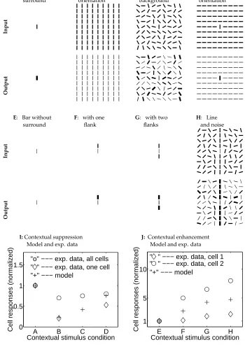
Fig. (3) shows that the model qualitatively replicates the results of physiological experiments on contextual influences from beyond the CRFs (Knierim and van Essen 1992, Kapadia et al, 1995). The suppression from surrounding textures in the model is strongest when the surround bars have the same orientation as the center bar, is weaker when the surround bars have random orientations, and is weakest when the surround bars have orthogonal orientations to the center bar. That the orthogonally oriented surround should lead to the weakest suppression is expected since the intra-cortical
Figure 3: (Caption for figure in previous page) Simulating the physiological experiments by Knierim and van Essen (1992) and Kapadia et al (1995) on con-textual influences to compare the model behavior with the experimental data. The model input stimuli are composed of a vertical (target) bar at the center surrounded by various contextual stimuli. All the visible bars have high con-trast input
except for the target bar in E, F, G, Hwhere
is near threshold. The input and output strengths are proportional to the bar widths with the same proportionality factors (one for the input and another for the output) across different subplots for direct comparison.A, B, C, D sim-ulate the experiments by Knierim and van Essen (1992) where a target bar is presented alone or is surrounded by contextual textures of bars oriented par-allel, randomly, or orthogonal to it, respectively. The responses to the (center) target bars inA, B, C, Dare, respectively,
,
,
(averaged over differ-ent random surrounds),
.E, F, G, H simulate the experiments by Kapadia et al (1995) where a low contrast (center) target bar is either presented alone or is aligned with some high contrast contextual bars to from a line with or with-out a background of randomly oriented high contrast bars. The responses to the target bars inE, F, G, Hare, respectively,
interactions only link bars preferring similar orientations, and is also the neural basis for pop out of a target bar among homogeneous background bars of a different orientation. Note that the response to the target bar is lower in Fig. (3D) than in Fig. (3A). That is, pop-out is manifested by having the responses to the target being higher than the responses to the background. Pop-out is not dependent on the responses to the target being higher in the face of one background than the responses to the target in the face of a different background — a target pops-out against a blank background as well.
The relative degree of suppression in the model is quantitatively comparable to physiologically measurements of orientation selective cells that are sensitive to orien-tation contrast (Knierim and van Essen 1992; denoted by the ‘ ’s in Fig. (3I)). When averaged over all cell types (the ‘o’s in Fig. (3I)), the suppression observed experimen-tally is quantitatively weaker than that in our model. One possible explanation for this discrepancy could be that the results in our model apply only to those pyramidal cells that are orientation selective, whereas in the experiment many different cell types were probably recorded, including some that are interneurons and some that are not even orientation selective (Knierim and van Essen 1992). Using just the same neural circuit, Figs. (3E,F,G,H, J) compare contextual facilitation with the corresponding physiological data (Kapadia et al 1995). This facilitation is expected on the basis of our “bow-tie” like connection pattern. The quantitative degree of response enhancement is different for the different cells recorded in the experiment, and varies with the input contrast level in our model.
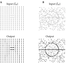
Given these results, we can then expect our model to perform appropriately on the sort of contour detection and pop-out tasks that are typically used in psychophysical studies (Fig. 4). Indeed, pop-out has recently been observed physiologically in V1 (Kastner et al 1997, Nothdurft et al 1998). Contour enhancement is built explicitly into the connection structure of the model. However, the contours can also be seen as where input homogeneity breaks down — here it is the statistical characteristics of the image noise in the background that are homogeneous.
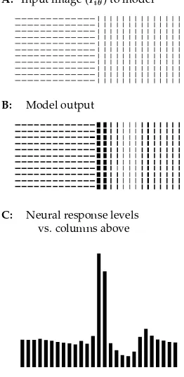
Fig. 5 shows how texture boundaries become highlighted. Fig. 5A shows a sam-ple input containing two regions. Fig. 5B shows the model output. Fig. 5C plots the responses (saliencies) to the bars averaged in each column in Fig. 5B, indicat-ing that the most salient bars are indeed near the region boundary. Fig. 5D confirms that the boundary can be identified by thresholding the output activities using a thresh-old,
, which is used to eliminates outputs that fire less strongly than the fraction
of the highest output max
in the image. Note that V1 does not perform such thresholding, it is performed in this paper only for the purposes of display. The value of the threshold used in each example has been chosen for optimal visualization. To quantify the relative salience of the boundary, define the net salience at each grid point as that of the most activated bar (max
), let be av-erage salience across the most salient grid column parallel to and near the boundary, and and be the mean and standard deviation in the saliencies of all locations. The relative salience of the boundary can be assessed by two quantities
and
(although these may be psychophysically incomplete as measures).
can be visualized from the thicknesses of the output bars in the figures, while mod-els the psychological
score. A salient boundary should give large values for
0
. In Fig. (5),
0
-
10
A Input (
)
Output
B Input (
)
Output
Figure 4:A:A small region pops out since all parts of it belong to the boundary. The response to figure is 2.42 times of the average response to the background. B:Exactly the same model circuit (and parameters) performs contour enhance-ment. The input strength is
. The responses to the contour segments are
, and to the background elements
.
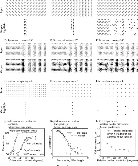
stronger when the texture elements on one side of them are parallel to the boundaries (Wolfson and Landy 1995), cf. Fig (6A) and Fig. (5). In fact, the model predicts that cells responding to bars near texture borders should be tuned to the orientation of the borders, and that the preferred border orientation should be the same as the preferred orientation of the bar within the CRF, as shown in Fig. (6L).
Fig (6) shows other examples demonstrating how the strength of the border high-light decreases with decreasing orientation contrast at the border, increasing orientation noise in the texture elements, or increasing spacing between the texture bars. When the orientation contrast is only , the boundary strength is very weak, with the bound-ary measures
0
/
A: Input image (
) to model
B: Model output
C: Neural response levels vs. columns above
D: Thresholded model output
Figure 5: An example of the segmentation performance of the model. A: In-put
consists of two regions; each visible bar has the same input strength. B: Model output forA, showing non-uniform output strengths (temporal
av-erages of
) for the bars. C: Average output strengths (saliencies) in a column vs. lateral locations of the columns inB, with the heights of the bars proportional to the corresponding bar output strengthes. D:The thresholded
output fromBfor illustration,
.
an orientation contrast at the texture border is more severely smeared by orientation noise. A further result of the noise is that orientation contrasts are created at locations
A:Border ori. contrast =
. B:Border ori. contrast =
. C:Border ori. contrast =
.
D:Texture ori. noise =
. E:Texture ori. noise =
. F:Texture ori. noise = .
G:texture bar spacing = 2. H:texture bar spacing = 3. I:texture bar spacing = 4.
J:performance vs. border ori. contrast.
Model and exp. data.
K:performance vs. texture bar spacings.
Model and exp. data.
L:Cell response vs.
relative border orienation. Model prediction.
Input
Output highlight
Input
Output
Input
Output highlight
0 20 40 60 80 50
75 100
Orientation contrast (degrees)
Percent correct "x, +" −− model
" , " −− exp. data without orientation noise
with ori. noise
0 5 10
0 1
Bar spacing / Bar length
Detectability
"+" −− model " , , " −− exp. data
0 20 40 60 80 0
0.2 0.4 0.6 0.8
Relative border orientation (degrees)
Cell response to bar
"+" −− model prediction given a 90 degree ori. contrast at the border
Figure 6:
In Fig.(6I), the texture elements are very sparse, and the boundary strengths are very weak
0
0 . By comparison, the denser texture elements in Fig.(6H) give a boundary with
0
Figure 6: (Caption for figure previous page) Model’s segmentation perfor-mance, comparison with psychophysical data, and a prediction. A, B, C, D, E, F, G, H, I:Additional examples of model performance in different stimulus configurations. Each is an input image as in Fig. 5A followed immediately below by the corresponding thresholded (strongest) model outputs as in Fig. 5D, or unthresholded model output as in Fig. 5B.A, B, Cshow the effects of orientation contrasts at the border.D, E, Fshow the effects of orientation noise in regions. The neighboring bars within one texture region differ in orientation by a random amount whose averages are respectively
,
, and
.G, H, I show the effects of texture bar spacing.J: segmentation performance versas ori-entation contrast at the border from the model, ‘+’ and ‘x’, and psychophysical behavior ‘ ’ and ‘ ’ from Nothdurft (1991). Data points ‘ ’ and ‘x’ are for cases without orientation noise, ‘ ’ and ‘+’ cases when the orientation noise amounts
to
on average between neighboring bars within one texture region (as inE). Given an orientation contrast, the data point ’+’ or ’x’ for the model is an aver-age of all possible relative orientations between the texture bars and the texture border. K: segmentation performance versas bar spacing from the model ‘+’ and psychophysical behavior ‘ ’, ‘o’, and ‘ ’ (each symbol for a particular bar length) from Nothdurft (1985). All data points are obtained from stimuli with a fixed orientation contrast
at the border and without orientation noise.L: Cell responses near a texture border versas relative orientations between the border and the bars within the CRFs. The plot is based on a fixed orientation contrast
at the border. The threshold used to obtain the output highlights in A, B, C, G, H, Iare, respectively,
.
higher than average, it has a high
score, i.e., the saliencies in the background are very homogeneous, making a difference very noticable. By contrast,
0 0
for Fig.(6F) — although the average salience of the boundary column is higher than the average, this difference is less significant with a
score
because the salience in the background is very inhomogeneous. To compare the performance of the network with psychophysical data (Nothdurft 1985, 1991), we model human behavior, in particular the measures ofPercentage of Correct ResponsesorDetectabilityin locating or detecting texture borders, as functions of the
score of the boundary strength.1 Fig
(6J,K) compares the behavior of the model with psychophysical data on how segmenta-tion performance depends on orientasegmenta-tion contrast, orientasegmenta-tion noise, and bar spacing.
Note also that the most salient location in an image may not be exactly on the
bound-1Let
, be the probability of getting a measurement below from a normal distribution. For psychophysical tasks in which subjects make binary judgements about the texture border, e.g., whether the border is oriented horizontally or vertically, the percentage of correct judgements is modeled by
! #"$&%(' *)*+ , where
is a parame-ter used to account for various human, random, and task specific factors, such as the number of possible locations in an image for the texture border that a subject expects. For detectability tasks, such as detecting and identifyng the shapes of texture borders, the detectability in the model is modeled analogously by,
.-0/21435146
7
% . This ranges in [0,1]. Parameter values
8 and
:9 are used for the two conditions (with and without orientation noise) in Fig (6J);
ary (Fig. 6B), or may be biased to one side of the boundary (Fig. (5B)). This should lead to a bias in the estimation of the border location, and can be experimentally tested. This is a hint that outputs from pre-attentive segmentation need to be processed further by the visual system.
A
B
C
D
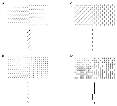
Figure 7: A, B, C: Model performance on regions with complex texture ele-ments, andD:regions with stochastic texture elements. Each plot is the model input (
) followed immediately below by the output (
) highlights. For A, B, C, Drespectively, the thresholds to generate the output highlights are
.
exactly the same features and would naturally be classified as the same texture. Seg-mentation in this case would be difficult if region boundaries were located by finding where texture classifications differ, as in traditional approaches to segmentation. Fig. 7C demonstrates that the model locates the correct border without being distracted by orientation contrast at locations within each texture region. The weakest boundary in Fig. (7) is that in Fig. (7B) with
0
0 , and the other three cases have
scores close to or higher than
.
The model works in these cases because it is designed to detect where input homo-geneity or translation invariance breaks down. In the example of Fig. 7C, any particular vertical bar within the right region and far enough away from the border, has exactly the same contextual surround as any other similarly chosen vertical bar, i.e, they are all within the homogeneous or translation invariant part of the region. Therefore none of such vertical bars will induce a higher response than any other since they have the same direct input and the same contextual inputs. The same argument applies to the oblique bars or horizontal bars far away from the border in Fig. 7C as well as in Fig. 7A,B. However, the bars at or near the border do not have the same contextual surround (i.e., contextual inputs) as those of the other bars, i.e., the homogeneity is truely broken. Thus they will induce different responses. By design, the border responses will be higher. In other words, the model, with its translation invariant horizontal connection pattern, only detects where input homogeneity breaks down, and the pattern complexity within a region does not matter as long as the region is homogeneous. Orientation (or feature) contrasts often spatially coincide with the breakdowns of input homogeneity. However, they should not be taken as thegeneralbasis for segmentation. The stochasticity of the bars in Fig. 7D results in a non-uniform response pattern even within each region. In this case, just as in the examples in Fig. (6)D,E, the border induces the highest responses because it is where homogeneity breaks most strongly.
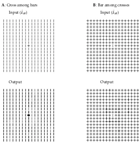
Our model also accounts for the asymmetry in pop-out strengths that is observed psychophysically (Treisman and Gormican, 1988), i.e., item A pops out among a back-ground of items B more easily than vice versa. Fig. (8) demonstrates such an example, in which a cross among bars pops out much more readily than a bar among crosses. The horizontal bar in the target cross (among background vertical bars) experiences no iso-orientation suppression, while the vertical target bar among the crosses experi-ences about the same amount of iso-orientation suppression as the other vertical bars in the background crosses and therefore is comparatively weaker. This mechanism is effectively a neural basis for the psychophysical theory of Treisman and Gelade (1980) which suggests that targets pop out if they are distinguished from the background by possessing at least one feature (e.g., orientation) that the background lacks, but that they will not pop out if they are distinguished only bylackinga feature that is present in the background. Other typical examples on visual search asymmetry in the literature can also be qualitatively accounted for by the model (Li 1998b, 1999). Such asymmetry is expected in our framework — the nature of the breakdown in homogeneity in the input, i.e., the arrangement of direct and contextual inputs on and around the target features, is quite different depending on which image item is the figure and which is the background.
A: Cross among bars Input (
)
Output
Input ( )
Output
B: Bar among crosses
Figure 8: Asymmetry in pop-out strengths.A: The response to the horizontal bar in the cross is 3.4 times that to the average background.B: The area near the central vertical bar is the most salient part in the image, but the neural responses there are no more than 1.2 times that in the average background. The target bar itself is actually a bit less salient than the average background.
texture border is correctly highlighted (together with some other conspicuous image locations). It is important to stress that this paper isolates and focuses on the role of the intracortical computation – the model’s performance, particularly on natural images, can only be improved using better methods of front-end processing, such as denser and multiscale sampling.
4 Summary and discussions
4.1 Summary of the results
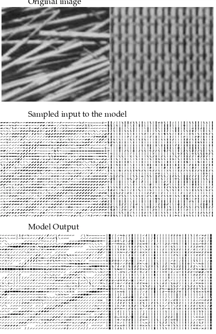
cap-Original image
Sampled input to the model
Model Output
Figure 9: The model performance on a photo input. The photo is sampled by even and odd CRFs whose outputs are combined to form the phase insensitive edge/bar input signals to the model pyramidal cells. At each grid point, bars
of almost all
orientations have nonzero input values
. For display clarity, no more than 2 strongest input or output orientations are plotted at each grid point in model input and output. The model input is much degraded from the photo through this sampling because of the sparse and single scale sampling in the model. The locations of highest responses include the texture border and some conspicous locations within each texture region. The image space has wrap around boundary condition. Some highlights in the outputs away from the boundary are caused by the finite size (of the texture regions) effect.
both the region boundary effect and contour enhancement — individual contours in a noisy or non-noisy background can also be seen as examples of the breakdown of homo-geneity in inputs. Our model suggests that V1, as a saliency network, has substantially more computational power than is traditionally supposed.
4.2 Relation to other studies
It has recently been argued that much texture analysis and segmentation are performed at low levels of visual processing (Bergen, 1991). The observed ease and speed of solv-ing many texture segmentation and target detection tasks have long led theorists to propose that the computations responsible for this performance must be pre-attentive (Treisman and Gelade 1980, Julesz 1981, Treisman and Gormician 1988). Correspond-ingly, many relevant models using low level and autonomous network mechanisms have been proposed.
To characterize and thus discriminate texture regions, some models use responses of image filters resembling the CRFs of the V1 cells (Bergen and Adelson 1988); others use less biologically motivated feature measures such as pixel correlations and histograms (Haralick and Shapiro, 1992).
Another class of models goes beyond the direct responses from the image filters and includes interactions between the filter or image units. The interactions in these models are often motivated by their cortical counterparts. They are designed to charac-terize texture features better and often help to capture context dependences and other statistical characteristics of texture features. Some of these models are based on Markov Random Field techniques (Haralick and Shapiro, 1992, Geman and Geman, 1984); oth-ers are closer to neurobiology. For instance, Caelli (1988) suggests a dynamic model in which the image filter units interact locally and adaptively with each other such that the ultimate responses converge to an “attractor” state characterizing the texture fea-tures. Interestingly, this dynamic interaction can make the feature outputs of a figure region dependent on the features of background regions, and was used (Caelli 1993) to account for examples of asymmetries between figure and ground observed by Gurnsey and Browse (1989). Malik and Perona’s model (1990) contains neural based multiscale filter (feature) units which inhibit each other in a form of winner-take-all competition which gives a single final output feature at each image location.
Many of these models capture well much of the phenomenology of psychophysical performance. They share the assumption that texture segmentation first requires char-acterizing the texture features at each image location. These feature measurements are then compared at neighboring locations (either by explicit interactions in the model, or, implicitly, by some unmodeled subsequent processing stage) to locate boundaries between texture regions.
There are also various related models which focus on the computation of contour enhancement. Li (1998a) presents a detailed discussion of them and their relation to the present model. In particular, a model by Grossberg and coworkers (Grossberg and Mingolla 1985, Grossberg et al 1997) proposes a “boundary contour system” as a model of intra-cortical and inter-areal neural interactions within and between V1 and V2. The model aims to capture illusory contours which link bar segments and line endings. Our model is the only one to models both contour enhancement and region boundary high-lights in the same neural circuit. Of course, its instantiation in V1 limits its power in some respects – it does not perform computations such as the classification and smooth-ing of region features and the sharpensmooth-ing of boundaries that are performed by certain other models (e.g., Malik and Perona 1990).
Since it locates conspicuous image locations without using filters that are specif-ically tuned to complex region features (such as the ‘+’s and ‘x’s in Fig. (7D)), our model reaches beyond early visual processing using such things as center-surround fil-ters (Marr, 1982). While the early stage filfil-ters code image primitives (Marr, 1982), our mechanism should help in the representations of object surfaces. Since contextual in-fluences are collected over whole neighborhoods, the model naturally accounts for the way that regions are defined by the statistics of their contents. This agrees with Julesz’s conjecture of segmentation by image statistics (Julesz, 1962) without imposing any re-striction that only the first and second order image statistics are important. Julesz’s concept of textons (Julesz, 1981) could be viewed in this framework as any feature to which the particular intra-cortical interactions are sensitive and discriminatory. Given the way that it uses orientation dependent interactions between neurons, our model agrees with previous ideas (Northdurft, 1994) that (texture) segmentation is primarily driven by orientation contrast. However the emergent network behavior is collective and accommodates characteristics of general regions beyond elementary orientations, as in Fig. 7. The psychophysical phenomena of filling-in (when one fails to notice a small blank region within a textured region) could be viewed in our framework as the instances when the network fails to sufficiently highlight the non-homogeneity in in-puts near the filled-in area.
Our pattentive segmentation is quite primitive. It merely segments surface re-gions, whether or not these regions belong to different visual objects. It does not char-acterize or classify the region properties or categories. In this sense, this pre-attention segmentation process is termed segmentation without classification (Li, 1998b). Hence, for example, our model does not say whether a region is made of a transparent sur-face on top of another sursur-face, nor does the model facilitate the pop-out process based on categorical informations such as the target being the only “steep” item in an image (Wolfe and Friedman-Hill 1992).
modula-tion in V1, especially those in figure surfaces (Zipser 1998, private communicamodula-tion), is strongly reduced or abolished by anaesthesia or lesions in higher visual areas (Lamme et al 1997), while experiments by Gallant et al (1995) show that activity modulation at texture boundaries is present even under anaesthesia.
Taken together, this experimental evidence suggests the following computational framework. Pre-attentive segmentation in V1 precedes region classification; region clas-sification following pre-attentive segmentation commences in higher visual areas; the classification is then fed back to V1 in the form of top-down influences which allows the segmentation to be refined (for instance, by removing the bias in the estimation of the border location in the example of Fig. 6B); this latter segmentation refinement pro-cess might be attentive and can be viewed as segmentation by classification. Finally, the bottom-up and top-down loop can be iterated to improve both classification and seg-mentation. Top-down and bottom-up streams of processing have been studied by many others (e.g., Grenander 1976, Carpenter and Grossberg 1987, Ullman 1994, Dayan et al, 1995). Our model studies the first step in the bottom up stream, which initializes the iterative loop. The neural circuit in our model can easily accommodate top-down feed-back signals which, in addition to the V1 mechanisms, selectively enhance or suppress neural activities in V1 (see examples in Li 1998a). However, we have not yet modeled how higher visual centers process the bottom up signals to generate the feedback.
4.3 Model predictions
The experimentally testable predictions of the model are: (1) cell responses should be tuned to the orientation of nearby texture borders (Fig. (6L)), and the preferred border orientation should be the same as that of the bar within the CRF; (2): the horizontal connection should have a qualitative “bow-tie” structure as in Fig. 2B, with a dominant monosynaptic excitation between cells tuned to similarly oriented and co-aligned bars and a dominant disynaptic inhibition between similarly oriented but not co-aligned bars; (3): there should be stimulus dependent biases in the border locations that could be estimated on the basis of the neural responses (e.g., Fig. 6B) or by pre-attentive vision.
4.4 Limitations and extensions of the model
Our model is still very primitive compared with the true complexity of V1. A particular lacuna is multiscale sampling. This is important, not only because images contain mul-tiscale features, but also because arranging for the model to treat flat surfaces slanted in depth as “homogeneous” or “translation invariant” requires some explicit mecha-nisms for interaction across scales. Merely replicating and scaling the current model to multiple scales is not sufficient for this purpose. In addition to orientation and spatial location, neurons in V1 are tuned for motion direction/speed, disparity, ocularity, scale, and color (Hubel and Wiesel 1962, Livingstone and Hubel 1984), and our model should be extended accordingly. The intra-cortical connections in the extended model will link edge segments with compatible selectivities to scale, color, ocular dominance, disparity, and motion directions as well as orientations, as suggested by experimental data (e.g., Gilbert 1992, Ts’o and Gilbert 1988, Li and Li 1994). The extended model should be able to highlight locations where input homogeneity in depth, motion, color, or scale is broken.
Other desirable extensions and refinements of the model include the sort of dense and over-complete input sampling strategy that seems to be adopted by V1, more pre-cisely determined CRF features, physiologically and anatomically more accurate intra-cortical circuits within and between hypercolumns, and other details such as on and off cells, cells of different CRF phases, non-orientation selective cells, end stopped cells, and more cell layers. These details should help to achieve a better quantitative match between the model and human vision.
Any given model, with its specific neural interactions, will be more sensitive to some region differences than others. Therefore, the model sometimes finds it easier or more difficult than humans to segment some regions. Physiological and psychophysical measurements of the boundary effect for different types of textures can help to constrain the horizontal connection patterns in an improved model. Experiments also suggest that the connections may be learnable or plastic (Karni and Sagi, 1991, Sireteanu and Rieth 1991, Polat and Sagi 1994).
We currently model salience at each location quite crudely, using just the activity of the single most salient bar. It is essentially an experimental question as to how the salience should best be defined, and the model can be modified accordingly. This will be particularly critical once the model includes multiple scales, non-orientation selective cells, and other visual input dimensions. The activities of cells in different channels need somehow to be combined to determine the salience at each location of the visual field.
In summary, this paper proposes that the contextual influences via intra-cortical in-teractions in V1 serve the purpose of pre-attentive segmentation. It introduces a simple, biologically plausible model which demonstrates this proposal. Although the model is as yet very primitive compared to the real cortex, our results show the feasibility of the underlying ideas, that simple pre-attentive mechanisms in V1 can serve difficult seg-mentation tasks, that breakdown of input homogeneity can be used to segment regions, that region segmentation and contour detection can be addressed by the same mecha-nism, and that low-level processing in V1 together withlocalcontextual interactions can contribute significantly to visual computations atglobalscales.
signifi-cantly improve the presentation of this paper, a reviewer for his/her comments, many other colleagues for their questions and comments during and after my seminars, and the Center for Biological and Computational Learning at MIT for hosting my visit. This work is supported in part by the Hong Kong Research Grant Council and the Gatsby Foundation.
References
[1] Albrecht D. G. and Mamilton D. B. (1982). Striate cortex of monkey and cat: Con-trast response function.J. Neurophysiol.Vo. 48, 217-237.
[2] Allman, J. Miezin, F. and McGuinness E. (1985) Stimulus specific responses from beyond the classical receptive field: neurophysiological mechanisms for local-global comparisons in visual neurons.Ann. Rev. Neurosci.8, 407-30.
[3] Bergen J.R. (1991) Theories of visual texture perception. In Vision and visual dys-functionD. Regan (Ed.) Vol. 10B (Macmillan),pp. 114-134.
[4] Bergen J. R. and Adelson, E. H. (1988) Early vision and texture perception.Nature 333, 363-364.
[5] Caelli, T. M. (1988) An adaptive Computational Model for Texture Segmentation.
IEEE trans. Systems, Man, and Cybern.Vol. 18, p9-17.
[6] Caelli, T. M. (1993) Texture classification and segmentation algorithms in man and machines.Spatial VisionVol. 7 p 277-292.
[7] Carpenter, G & Grossberg, S (1987). A massively parallel architecture for a self-organizing neural pattern recognition machine.Computer Vision, Graphics and Image Processing,37, 54-115.
[8] Cavanaugh, J.R., Bair, W., Movshon, J. A. (1997) Orientation-selective setting of contrast gain by the surrounds of macaque striate cortex neuronsSoc. Neuroscience Abstract227.2.
[9] Dayan, P, Hinton, GE, Neal, RM & Zemel, RS (1995). The Helmholtz machine.
Neural Computation,7, 889-904.
[10] Douglas R. J. and Martin K. A. (1990) Neocortex, inSynaptic Organization of the BrainG. M. Shepherd. (ed). Oxford University Press, 3rd Edition, pp389-438 [11] Eckhorn, R. Bauer R., Jordan W., Brosch M., Kruse W., Munk M., and Reitboeck H.
J. (1988) Coherent oscillations: a mechanism of feature linking in the visual cortex? Multiple electrode and correlation analysis in the cat.Biol. Cybern. 60, 121-130. [12] Field D.J., Hayes A., and Hess R.F. (1993). Contour integration by the human visual
system: evidence for a local ‘associat ion field’Vision Res.33(2): 173-93.
[13] Fitzpatrick D. (1996) The functional organization of local circuits in visual cortex: Insights from the study of tree shrew striate cortex.Cerebral Cortex, V6, N3, 329-341. [14] Gallant, J. L. , van Essen, D. C. , and Nothdurft H. C. (1995) Two-dimensional and three-dimensional texture processing in visual cortex of the macaque monkey. In
Early vision and beyondT. Papathomas, Chubb C, Gorea A., and Kowler E. (eds). MIT press, pp 89-98.
[16] Gilbert, C. D. (1992) Horizontal integration and cortical dynamicsNeuron.9(1), 1-13.
[17] Gilbert C.D. and Wiesel T.N. (1983) Clustered intrinsic connections in cat visual cortex.J Neurosci.3(5), 1116-33.
[18] Gilbert C. D. and Wiesel T. N. (1990) The influence of contextual stimuli on the orientation selectivity of cells in primary visual cortex of the cat.Vision Res30(11): 1689-701.
[19] Gray C. M. and Singer W. (1989) Stimulus-specific neuronal oscillations in orienta-tion columns of cat visual cortexProc. Natl. Acad. Sci. USA86, 1698-1702.
[20] Grenander, U (1976-1981).Lectures in Pattern Theory I, II and III: Pattern Analysis, Pattern Synthesis and Regular Structures.Berlin: Springer-Verlag., Berlin.
[21] Grossberg S. and Mingolla E. (1985) Neural dynamics of perceptual grouping: tex-tures, boundaries, and emergent segmentationsPercept Psychophys.38(2), 141-71. [22] Grossberg S. Mingolla E., Ross W. (1997) Visual brain and visual perception: how
does the cortex do perceptual grouping?TINSvo. 20. p106-111.
[23] Gurnsey, R. and Browse R. (1989) Asymmetries in visual texture discrimination.
Spatial Vision4. 31-44.
[24] Heeger D. J. (1992) Normalization of cell responses in cat striate cortex.Visual Neu-rosci.9, 181-197.
[25] Haralick R. M. Shapiro L. G. (1992) Computer and robot vision Vol 1. Addison-Weslley Publishing.
[26] Hirsch J. A. and Gilbert C. D. (1991) Synaptic physiology of horizontal connections in the cat’s visual cortex.J. Neurosci. 11(6): 1800-9.
[27] Hubel D. H. and Wiesel T. N. (1962) Receptive fields, binocular interaction and functional architecture in the cat’s visual cortex.J. Physiol. 160, 106-154.
[28] Julesz, B. (1962) Visual pattern discriminationIRE Transactions on Information theory IT-884-92.
[29] Julesz, B. (1981) Textons, the elements of texture perception and their interactions.
Nature290, 91-97.
[30] Kapadia, M. K., Ito, M. , Gilbert, C. D., and Westheimer G. (1995) Improvement in visual sensitivity by changes in local context: parallel studies in human observers and in V1 of alert monkeys.Neuron.15(4), 843-56.
[31] Karni A, Sagi D. (1991) Where practice makes perfect in texture discrimination: evidence for primary visual cortex plasticity.Proc. Natl. Acad. Sci. USA88 (11): 4977.
[32] Kastner S., Nothdurft H-C., Pigarev I.N. (1997) Neuronal correlates of pop-out in cat striate cortex.Vision Res.37(4), 371-76.
[33] Knierim J.J. and van Essen D. C. (1992) Neuronal responses to static texture pat-terns ion area V1 of the alert macaque monkeys.J. Neurophysiol.67, 961-980. [34] Kovacs I. and Julesz B. (1993) A closed curve is much more than an incomplete
one: effect of closure in figure-ground segmentation.Proc Natl Acad Sci USA. 15; 90(16): 7495-7.
[36] Lamme V. A. F., Zipser K. and Spekreijse H. (1997) Figure-ground signals in V1 depend on consciousness and feedback from extra-striate areasSoc. Neuroscience Abstract603.1.
[37] Levitt J. B. and Lund J. S. (1997) Contrast dependence of contextual effects in pri-mate visual cortex.Nature387(6628), 73-6.
[38] Li, Zhaoping (1997) Primary cortical dynamics for visual grouping inTheoretical aspects of neural computationWong, K.Y.M, King, I, and D-Y Yeung, (Eds), page 155-164. Springer-Verlag, Hong Kong.
[39] Li, Zhaoping. (1998a) A neural model of contour integration in the primary visual cortex.Neural Computation10(4) p 903-940.
[40] Li, Zhaoping (1998b) Visual segmentation without classification: a proposed func-tion for primary visual cortex.Perceptionvol. 27, supplement, p.45.
[41] Li, Zhaoping (1999) “A V1 model of pop out and asymmetry in visual search” to appear inAdvances in neural information process systems 11, Kearns, M.S., Solla S.A., and Cohn D. A. Eds. MIT Press.
[42] Li, C.Y., and Li, W. (1994) Extensive integration field beyond the classical receptive field of cat’s striate cortical neurons — classification and tuning properties.Vision Res. 34(18), 2337-55.
[43] Livingstone M. S. and Hubel, D. H. (1984) Anatomy and physiology of a color system in the primate visual cortex.J. Neurosci.Vol. 4, No.1. 309-356.
[44] Malik J. and Perona, P. (1990) Preattentive texture discrimination with early vision mechanisms.J. Opt. Soc. Am. A7(5),923-932.
[45] Marr D. (1982)Vision, A computational investigation into the human representation and processing of visual information. Freeman.
[46] Merigan W. H. Mealey T.A., Maunsell J. H. (1993) Visual effects of lesions of cortical area V2 in macaques.J. Neurosci133180-91.
[47] Nothdurft H. C. (1985) Sensitivity for structure gradient in texture discrimination tasks.Vis. Res.Vol. 25, p 1957-68.
[48] Nothdurft H. C. (1991) Texture segmentation and pop-out from orientation con-trast.Vis. Res.Vol. 31, p 1073-78.
[49] Nothdurft H. C. (1994) Common properties of visual segmentation. inHigher-order processing in the visual systemBock G. R., and Goode J. A. (Eds). (Wiley & Sons), pp245-268
[50] Nothdurft H-C., Gallant J.L. Van Essen D. C. (1998). Response modulation by tex-ture surround in primate area V1: correlates of ‘pop-out’ under anesthesia.Visual Neurosci.in press.
[51] Nothdurft H-C. Different approaches to the coding of visual segmentation. in Com-putational and psychophysical mechanisms of visual coding, Eds. L. Harris and M. Kjenkius, Cambridge Unviersity Press, New York, 1997.
[52] Polat U. Mizobe K. Pettet M. Kasamatsu T. Norcia A. (1998) Collinear stimuli reg-ulate visual responses depending on cell’s contrast threshold.Naturevol. 391, p. 580-583.
[54] Polat U. and Sagi D. (1994) Spatial interactions in human vision: From near to far via experience-dependent cascades of connections.Proc. Natl. Acad. Sci. USA91. p1206-1209.
[55] Rockland K. S. and Lund J. S. (1983) Intrinsic Laminar lattice connections in pri-mate visual cortex.J. Comp. Neurol.216, 303-318
[56] Scialfa C. T. and Joffe K. M. (1995) Preferential processing of target features in tex-ture segmentation.Percept Psychophys57(8). p1201-8.
[57] Sillito, A. M. Grieve, K.L., Jones, H.E. Cudeiro, J. and Davis J. (1995) Visual cortical mechanisms detecting focal orientation discontinuities.Nature378(6556), 492-6. [58] Sireteanu R. and Rieth C. (1992). Texture segregation in infants and children.Behav.
Brain Res.49. p. 133-139
[59] Somers, D. C., Todorov, E. V., Siapas, A. G. and Sur M. (1995) Vector-based inte-gration of local and long-range information in visual cortex.A.I. Memo. NO. 1556,
MIT.
[60] Stemmler M, Usher M, Niebur E (1995) Lateral interactions in primary visual cor-tex: a model bridging physiology and psychophysics.Science269, 1877-80. [61] Treisman A. and Gormican S. (1988) Feature analysis in early vision: evidence for
search asymmetries.Psychological Rev.95, 15-48.
[62] Treisman A, and Gelade, G. A feature integration theory of attention.Cognitive Psychology12, 97-136, 1980.
[63] Ts’o D. and Gilbert C. (1988) The organization of chromatic and spatial interactions in the primate striate cortex.J. Neurosci.8: 1712-27.
[64] Ullman, S (1994). Sequence seeking and counterstreams: A model for bidirectional information flow in the cortex. In C Koch and J Davis, editors,Large-Scale Theories of the Cortex. Cambridge, MA: MIT Press, 257-270.
[65] Weliky M., Kandler K., Fitzpatrick D. and Katz L. C. (1995) Patterns of excitation and inhibition evoked by horizontal connections in visual cortex share a common relationship to orientation columns.Neurons15, 541-552.
[66] White E.L. (1989)Cortical circuitsBirkhauser.
[67] Wolfe J. M. and Friedman-Hill S. R. (1992) Visual search for oriented lines: The role of angular relation between targets and distractors.Spatial VisionVol. 6., p 199-207. [68] Wolfson S. and Landy M. S. (1995) Discrimination of orientation-defined texture
edges.Vis. Res.Vol. 35, Nl. 20, p 2863-2877.