A SEQUENTIAL ALGORITHM FOR SIGNAL
SEGMENTATION
Paulo Hubert ([email protected]) *
1, Linilson Padovese ([email protected])
2and Julio Stern ([email protected])
11
Instituto de Matematica e Estatistica - University of Sao Paulo (IME-USP)
2
Escola Politecnica - University of Sao Paulo (EP-USP)
* Corresponding author
Abstract
The problem of event detection in general noisy signals arises in many applications; usually, either a functional form for the event is available, or a previous annotated sample with instances of the event that can be used to train a classification algorithm. There are situations, however, where neither functional forms nor annotated samples are available; then it is necessary to apply other strategies to separate and characterize events. In this work, we analyze 15 minute-long samples of an acoustic signal, and are interested in separating sections, or segments, of the signal which are likely to contain significative events. For that, we apply a sequential algorithm with the only assumption that an event alters the energy of the signal. The algorithm is entirely based on Bayesian methods. Keywords signal processing; bayesian methods; subaquatic audio; hydrophone; unsupervised learning
1
Introduction
Signal processing is a field of intense research, both in engineering, physics and medicine1, and in the statistical and MAXENT literature[Bretthorst (1988)] [Jaynes (1987)] [Ruanaidh (1996)]. The most recurrent problems in the field are signal estimation, model comparison, and signal detection [Bretthorst (1990A)] [Bretthorst (1990B)] [Bretthorst (1990C)]: in signal estimation, given a func-tional form for the signal (for instance, an exponentially decaying tonal model) and a (discretized) sample, the researcher wants to estimate the functional form’s parameters (the rate of decay, the fundamental frequency). In model comparison, there are different possible functional forms for the signal, and given one or more samples, one is interested in selecting the most adequate model. In signal detection, the researcher is given a sample of the signal, and must decide if a given functional form (which we might call anevent) is or is not present.
These situations arise tipically when the researcher has some control over the process of data acquisition. Namely, she usually is well aware of the presence of the event of interest in the sample, or knows precisely the kind of event she is looking for (and / or its duration). In these situations, previous works from the 1980s and 1990s [Jaynes (1987)] [Bretthorst (1990A)] [Bretthorst (1990B)] [Bretthorst (1990C)] have succesfully applied maximum entropy and Bayesian methods to solve the basic problems of signal estimation, model comparison and signal detection.
On the other hand, there are situations in which the researcher has very little information about the occurrence times or precise functional form of events. This is the case in this work.
We analyze samples of a subaquatic audio recording obtained by the OceanPod, a hydrophone developed by the Laboratory of Acoustics and Environment (LACMAM) at EP-USP. The OceanPod is capable of storing 5 months of a digital signal sampled with a frequency of 11.025 Hz2.
In january, 2015, one OceanPod was first installed in the region of Parque da Laje, a marine conservation park in the brazilian coast, in the region of Santos, SP. It is kept at a depth of 20 meters, and after a period ranging from 30 to 90 days it is retrieved for data extraction. After the
1For a quick and interesting exposition on the applications of signal processing, see
https://signalprocessingsociety.org/our-story/signal-processing-101. For subacquatic signal processing, see [Etter (2013)].
2More information about the OceanPod can be found athttp://lacmam.poli.usp.br/Submarina.html
data is extracted, the hydrophone is reinserted at the same spot. Several of these data acquisition operations have been made from 2015 to the present time, and are still occurring.
When analyzing such data, one has very little information to work with. There is no exhaustive list of possible events that might be taking place, neither there is information about starting times or duration of their occurrences. If the analyst is looking for a very specific event (in terms of functional form either in time or frequency domain), it might be possible to design a (unsupervised) detection algorithm tailored to this functional form; even so, however, the lack of information about the starting times of the events make the detection task very computationally intensive, given the sparsity of subaquatic acoustic events [Hubert (2017)].
A natural approach is then to, first and foremost, separate sections from the signal that are likely to contain some event (as opposed to sections containing noise only). The underwater oceanic environment is very economic in this sense: there can be periods of many minutes (even hours) where nothing but the waves (and the omnipresent sound of shrimps and barnacles clapping and clicking) can be heard. This indicates that, rather than processing the entire signal in search of an event, it would be much better to first obtain sections where we believe something is happening, and then try to figure out exactly what it is.
This problem is known in the literature as signal segmentation, and shows up in different contexts [Makowsky (2014)] [Ukil (2006)] [Schwartzman (2011)] [Kuntamalla (2014)]. In the specific context of audio segmentation, [Theodorou (2014)] presents a review of the algorithms often applied to solve this problem. These are divided in three categories: the distance-based segmentation, the model-based segmentation, and hybrid techniques. The distance-based approach works directly with the audio waveform (amplitudes in time domain), and assumes nothing about the forms of the segments; the model-based segmentation, on the other hand, starts with a collection of models, and works by training a classification algorithm on previously annotated data. The hybrid approach applies both distance-based and model-based approaches in a single framework.
In this paper we propose an algorithm that can be classified as distance-based, in the sense that it does not assume a collection of models, nor does it use any pre-annotated samples. We formulate the problem in a very general form, and adopt a maximum entropy Bayesian approach to propose a solution. We argue that this theoretical framework is specially adequate for the situation of scarce information, since from maximum entropy we learn how to avoid insidious and implicit assumptions to sneak into the model, and from Bayesian inference we learn how to make the best use of whatever prior information is available.
Also, the maximum entropy Bayesian approach allows us to work from first principles, avoiding the introduction ofad hoc procedures. We work our way from the assumptions to the final method of solution, using little more than the basic theorems of probability theory, and making explicit each and every assumption we make about the signal we are analyzing.
The rest of the paper is organized as follows: in the next section, we introduce our main as-sumption and build the first part of the segmentation procedure. Section 3 completely defines our segmentation algorithm. Section 4 compares our algorithm with an alternative method found in the literature, using simulated data, and section 5 does the same comparison in a few samples from the actual signal obtained from the OceanPod. Section 6 concludes the paper.
2
Bayesian model for power switch
Suppose we are given a discretely sampled signal y∈ <N
corrupted with noise. Given a sampling frequency ratefs, this signal corresponds to a total duration ofT =N·fsseconds. We assume that the signal is stationary with 0 mean amplitude,E(yt) = 0, and finite powerV ar(yt) =σ02<∞. We adopt the notationyt to indicate thetcomponent of the discrete-time signal.
Now let’s imagine that, at sample time ¯t∈ {0, ..., T}, some event has started. Our only assumption is that, whatever the particular nature of this event, it causes a change in the total signal power; this is a rather reasonable assumption, since for the combination of two random variables to have the same variance as one of its components, it is necessary that the variables have an exact covariance ofσ21/2, whereσ21 is the variance of either one of the variables.
If we assume only that the signal has 0 mean amplitude and finite power, the maximum entropy principle leads us to choose a Gaussian probabilistic model for y [Jaynes (1987)]. The maximum entropy principle indicates that, given what is known about a random variable, one must choose the probabilistic model p that maximizes the entropyH(p) =−R
In our case, assuming the change of variance att= ¯t, we write the model
yt∼ (
N(0, σ02) ift≤¯t
N(0, δσ20) ift >¯t
(1)
The parameterδrepresents the ratio between the variances of the two signal sections or segments. Our goal is to estimate the value of ¯t, the starting time of the event. To accomplish that, we start by writing the likelihood
L(¯t, σ20, δ|y) = (2πσ 2 0)
−N
2δ−
N−¯t
2 exp " − P¯t t=1y 2 t 2σ2
0
−
PN t=¯t+1y
2 t 2δσ2
0 #
(2)
To keep our model as general as possible, we do not assume any prior information aboutδ (i.e., we do not know anything about the SNR of the possible events). In Bayesian terms, this ammounts to adopting a non-informative (improper) uniform prior for δ. Using this prior, we are able to analitically integrate equation 2 and obtain
L(¯t, σ02|y) = Z ∞
0
L(¯t, σ02, δ|y)dδ (3)
∝
" PN t=¯t+1y
2 t 2σ2
0
#−(N−¯t−6)
2
Γ
N−¯t−2 2
exp
"
−
P¯t t=1y
2 t 2σ2
0 #
(4)
If the variance of either segment is known, the above equation can be used directly to obtain the posterior distribution for ¯t. Ifσ2
0 is unknown, we must choose a prior distribution for it. We will not assume any particular knowledge about the variance; to keep the model invariant with relation to reparametrizations of this parameter, we adopt the Jeffreys’ prior [Jaynes (1968)] [Jeffreys (1946)]
π(σ0) = 1/σ0, and again integrate the above equation analitically to arrive at
L(¯t|y) = Z ∞
0
L(¯t, σ02|y)π(σ0)dσ0 (5)
∝ N X t=¯t+1
yt2
−(N−2¯t−6) Γ
N−¯t−2 2
¯t X
t=1
yt2 !−
(¯t+6) 2
Γ ¯
t+ 6 2
(6)
From this point, it is only necessary to pick a priorπt(t) for ¯t, multiply it by the above quation, and obtain (the kernel of) the posterior distribution for ¯t:
P(¯t|y)∝π(¯t)·
¯ t X
t=1
yt2 !−
(¯t+6)
2
N X
t=¯t+1
yt2
−(N−2t¯−6)
× (7)
Γ ¯
t+ 6 2
Γ
N−¯t−2 2
(8)
This gives us a discrete distribution with support over 1<¯t < N−1; this means that it is possible to calculate exactly the normalization constant that would make 7 a proper probability distribution. If we need to estimate ¯t, on the other hand, we can optimize equation 7 by inspection to find the MAP (Maximum a Posteriori) estimate.
In the next figures we present the distribution in 7 calculated over a simulated (Gaussian) signal of sizeN= 9000, with δ∈ {1.1,1.5,2}, ¯t∈ {N/3, N/2,2N/3}andσ0 = 1, and assuming a uniform prior over{2, N−2}for ¯t.
Figure 1: Posterior distribution for ¯t,δ= 1.1 (horizontal axis isi, index of signal vector; vertical axis is the posterior value)
Figure 3: Posterior distribution for ¯t, δ= 2 (horizontal axis isi, index of signal vector; vertical axis is the posterior value)
The model for the segmentation, as defined above, works well when the signal has one cut point. In most signals, however, and certainly on the samples from the OceanPod, there will be more than one segmentation point (i.e., more than one change of signal total power).
It would be straigthforward to generalize the above model to these situations, obtaining a posterior distribution for (¯t1,¯t2, ...,¯tk). However, the complexity of the discrete optimization problem involved with the MAP estimation of the cut points would grow exponentially. Also, it would be necessary to treat the new parameterk, the number of cutting points (or, equivalently, the number of segments in the signal), which we would like to avoid since we do not know this number in advance, and estimating it would be demanding3.
Instead, we observe that the MAP estimate calculated from the above posterior will tend to divide the signal in regions with maximally different powers. So, whenever there is more than one change of power along the signal sample, it would still tend to estimate the cutting point at the beginning or end of one segment. To illustrate our point, we simulate a signaly∈ <10000
with two cutting points, in two different situations: first, we change the signal power fromσ0= 1 toσ1= 2 att= 2000, and then back toσ0 at t= 5000; in the second figure, we change the power att= 6000 and then back to the original power att= 8000. The simulated signal, along with the cutting points estimated by maximizing the posterior distribution, are shown in figure 4 below.
Figure 4: Segmentation point estimated for signal with two power changes; see text for details
This observation suggests a recursive approach for automatic signal segmentation: we first
esti-3This new parameter is directly related to the dimensionality of the parametric space. Estimating this kind of parameter
mate one cutting point, and divide the original signalyin two segments,y1 andy2. We then apply again the same estimation to the new signalsy1 andy2, and so on. We repeat this procedure until some stopping criterion is met. This strategy gives rise to the sequential segmentation algorithm, which we define next.
3
The sequential segmentation algorithm
We define the sequential segmentation algorithm as follows:
(Sequential segmentation algorithm) Define the function seg(
y
∈ <
N,
n
min)
as:
1. If N < nmin, stop, returning the empty vectort= [];
2. Else
(a) Obtain the MAP estimate ¯t;
(b) Definey1=y1,...,¯t andy2=y¯t+1,...,N;
(c) (Stopping criterion)If var(y1) =var(y2), stop, returning the empty vectort= []; (d) Elsereturn the concatenated vector [seg(y1, nmin) t¯ ¯t+seg(y2, nmin)].
Please note that theseg appearing in the last line refers to the function itself; our algorithm, then, is of a recursive nature.
This recursive algorithm will output an ordered vectorτ∈[1, ..., N−1]kwith the starting points ofksignal segments, where the segments have been found to exhibit different powers. The condition
N ≥ nmin guarantees that the algorithm stops and is well defined; the main question is how to decide ifvar(y1) =var(y2), i.e., to define the stopping criterion.
As it is clear from the definition, the matter is one of testing the hypothesis of equality of variances, given two samples with mean 0. Or, using our parametrization, to test the hypothesisH0:δ= 1.
Our model is defined in the parametric space Θ =<+× <, whereθ= (σ02, δ); underH0, we have Θ0=<+. Our hypothesis thus lies in a subspace of Θ, i.e., it is asharp hypothesis.
The traditional statistical literature proposes a few different ways to test equality of variances, the most known being possibly theF test, and the likelihood ratio test. However, it is well reported that the traditional, frequentist tests, have a few drawbacks, related in particular to the definition of the alternative hypothesis [Good (1992)], or with the choice of an appropriate significance level for the decision function [Perez (2014)] [Pereira (1993)]. The classical Bayesian alternative would then be a Bayes factor test, which in turn would meet some difficulties with the fact that our null hypothesis defines a lower dimensional parametric space [Pereira (1999)].
A full bayesian procedure is available, however, that is well suited to the test of sharp hypothesis such asH0:δ= 1; this is the now well-knownfull bayesian significance test(FBST) of Pereira and Stern [Pereira (1999)]. This procedure works in the full parametric space, defining an evidence mea-sure based on thesurprise setof points having higher posterior density than the supremum posterior underH0. The test avoids altogether the imposition of positive probabilities over null measure sets such as Θ0 :{(δ, σ0)∈ <2 :δ= 1}, and has been tested many times with very good results (for a few examples see [Chakrabarty (2017)] [Hubert (2009)] [Lauretto (2009)] [Stern (2002)]).
Of course, even with the application of the FBST, there remains the problem of defining a decision function over the evidence value forH0,ev(H0, y); as we will see, however, this decision function will become trivial when we calibrate our testing procedure with the use of appropriate priors.
Recalling the probabilistic model of our signal, given yand ¯t, and definingy1 andy2 as in the above algorithm, we write the full posterior
P(d, s|y1, y2)∝πδ(d)πσ(s)(2πs2) −n1 +n2
2 d−
n2 2 exp − Pn1 t=1y 2 1,t 2s2 −
Pn2
t=1y 2 2,t 2ds2
(9)
wheren1 andn2 are the corresponding dimensions ofy1 andy2,πδ is the prior forδ andπσ the prior forσ0.
To incorporate the lack of knowledge about the base signal varianceσ0, and at the same time to guarantee invariance, we adopt again a Jeffreys’ priorπσ(s) = 1/s.
To define this prior, we consider what we do know about δ. We reason in the following terms: suppose we are to pick at random two contiguous sections of our signal, with sizesn1andn2; suppose that these sections haves1 ands2 as their respective powers, as estimated from the data. We then defineδ=s2
s1.
Now, unless we happen to pick by chance two segments that include a true change of power (in our terms, the beginning or end of an event), we expectδ to be very close to 1. This belief would be as strong as our perceived probability of finding an event at random in our signal. As we have mentioned before, the ocean’s subacquatic soundscape is a rather minimalist environment, with long periods of very low or no activity. So we believe that, in our thought experiment above, we are very likely to pick sections withδvery close to 1.
However, if we happen to pick a segment with an event, then we can expect to findδ >>1, since most events in our signal have large SNR values (for instance, the already mentioned boat engines, running at a small distance from the hydrophone). It is then reasonable to believe that, even though
δ is likely close to 1, it can sometimes differ significantly and assume high values, close toδ= 2 or even higher.
All of these considerations lead us to pick a prior distribution onδ that is: (a) centered around 1; (b) high-peaked around this same value; but (c) with larger tails than the Gaussian. Further on, to keep matters as simple as possible, we would like our prior to have few parameters (since we will use these parameters for the calibration of our algorithm). Combining all of these objectives, we propose a Laplace prior forδ:
πδ(d) = 1
βe
−|d−β1|
(10)
In practical terms, this prior will tend to favorH0 :δ= 1, inversely with the value ofβ. This value can be used as a calibration parameter for the detection algorithm. Also, picking a sufficiently low value forβwill guarantee a minimum prior probability for the meaningless situationδ≤0.
Again, we must stress that in working with acoustic signals with a sampling rate as high as 11 kHz, we will be dealing with large sample sizes; tipically we will define a smallest detectable event as a segment with a duration of around 1s, which means that we will be comparing the variances of samples with sizesN = 11025 each. On the other extreme, the algorithm will start with a signal of duration in the order of minutes (the files obtained from the hydrophone are configured as 15 minutes long for default), which translates to sample sizes in the order of millions. Our numerical tests indicate that the value ofβmust be set correspondingly; our best results usedβ∝10−5, as we will see in the results section.
With the model completely specified, the evidence value forH0is calculated as
ev(H0, y) = Z
T(y)
P(σ0, δ|y)dσ0dδ (11)
where
T(y) ={(σ0, δ)∈Θ :P(σ0, δ|y)> supΘ0P(σ0, δ|y)} (12)
It is noteworthy that, when defining the posterior for the cutting point ¯t, we chose priors for all the other parameters in order to analitically integrate them out. The intention behind this decision was to keep this step of the algorithm as simple as possible, since MAP estimation in this case is a discrete optimization problem which we solve by brute force. Now, however, when calculating the evidence for the hypothesisδ= 1, we want to work on the full parametric space, without explicitly marginalizing any parameter. This is the standard procedure when working with the FBST [Pereira (1999)].
To calculate the above integral, then, we adopt a numerical procedure: we apply a block Metropolis-Hastings algorithm, with a sample size of 10000 points after a burnin of another 10000 points, and using exponential distributions as candidates for bothσandδ.
The stopping criterion for the algorithm is finally defined by setting a minimal evidence forH0,
αmin; the algorithm will keep segmentating the signal as long as the evidence forH0:δ= 1 is lower than this threshold value:
(Stopping criterion) Given
y
1,
y
2and
α
min:
1. Obtains0=supΘ0P(σ0, δ|y);
2. Obtain the evidenceev(H0, y) =RT(y)P(σ0, δ|y)dσ0dδ;
One step of the full algorithm is shown schematically on the diagram in figure 5. Starting with a given signal, we first obtain the MAP estimate for ¯t, optmizing by inspection the posterior for the change point t. After estimating ¯t, we generate two segments, and use the FBST (via MCMC sampling of the full posterior) to test the hypothesisH0 :δ= 1.
Figure 5: One step of the sequential segmentation algorithm
4
Results: simulated signal
To test the performance of our algorithm we first apply it to simulated data. We simulatey∈ <20000, whereyt∼ N(0, σ2i), and we define 5 segments in the signal, given by the following definition for the varianceσ2
i:
σi2=
1 ifi≤5000
1.1 if 5000< i≤10000 1 if 10000< i≤12000 1.5 if 12000< i≤15000 1 ifi >15000
(13)
As a baseline method to use for comparison, we adopt the peak detection algorithm of Palshikar [Palshikar (2009)]. This algorithm defines peaks in the signal by using local and global properties. The local properties are based in functions calculated over windows of width k, centered around each coordinate of the signal. Each function reflects a different characterization of what actually constitutes a peak. The global properties arise when each peak is compared to the average amplitude of all peaks, and a thresholding is applied based on their standard deviation.
Palshikar’s algorithm takes then 2 parameters: h, the number of standard deviations to use as threshold, andk, the length of the window. Also the algorithm can use many different functions to define a peak locally; we run Palshikar’s algorithm using his threeS functions. The first function,
and the average of its left neighbouts, the signed difference between yt and the average of its right neighbours, and takes the mean4.
In table 1 we compare the results of our method with Palshikar’s algorithm, using each of the three
S functions and 8 combinations of values forhandk. For the sequential segmentation algorithm, we setβ∈ {1,0.01}andα∈ {0.01,0.1}; lower values ofβ imply higher prior weight to the hypothesis
δ = 1, while lower values ofαimply earlier stop for the algorithm (i.e., we require higher evidence againstδ= 1 to keep segmentating the signal). In the table, we labeled our algorithm asSeqSeg.
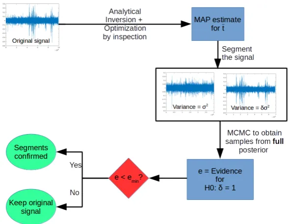
Algorithm Parameters Elapsed time (s) # of segments First cutting point Last cutting point
SeqSeg β= 1, α= 0.01 9.8912 5 4990 15001
SeqSeg β= 0.01, α= 0.01 11.8567 5 4990 15001
SeqSeg β= 1, α= 0.1 12.7605 5 4990 15001
SeqSeg β= 0.01, α= 0.1 11.5746 5 4990 15001
PalshikarS1 h= 3, k= 100 0.3116 31 4778 14852
PalshikarS2 h= 3, k= 100 0.3303 13 5039 14470
PalshikarS3 h= 3, k= 100 0.3443 9 1608 14249
PalshikarS1 h= 3, k= 500 0.4264 5 5039 14179
PalshikarS2 h= 3, k= 500 1.4768 55 1608 19892
PalshikarS3 h= 3, k= 500 1.3090 25 964 19892
PalshikarS1 h= 3, k= 1000 1.0846 16 964 19892
PalshikarS2 h= 3, k= 1000 1.2406 10 964 19892
PalshikarS3 h= 3, k= 1000 1.4050 55 1608 19892
PalshikarS1 h= 3, k= 2000 0.9451 25 964 19892
PalshikarS2 h= 3, k= 2000 0.9889 16 964 19892
PalshikarS3 h= 3, k= 2000 1.1212 10 964 19892
PalshikarS1 h= 4, k= 100 0.1718 5 13171 14311
PalshikarS2 h= 4, k= 100 0.2303 3 13171 14311
PalshikarS3 h= 4, k= 100 0.3023 4 12606 14727
PalshikarS1 h= 4, k= 500 0.4439 3 12606 14727
PalshikarS2 h= 4, k= 500 0.8924 16 1608 14923
PalshikarS3 h= 4, k= 500 0.9922 10 1608 14923
PalshikarS1 h= 4, k= 1000 1.0793 9 1608 14727
PalshikarS2 h= 4, k= 1000 1.2486 6 1608 14311
PalshikarS3 h= 4, k= 1000 0.8439 16 1608 14923
PalshikarS1 h= 4, k= 2000 0.9167 10 1608 14923
PalshikarS2 h= 4, k= 2000 1.0030 9 1608 14727
PalshikarS3 h= 4, k= 2000 1.1367 6 1608 14311
Table 1: Test results; see text for details
The experimental results show that our algorithm is much more robust than the peak detection algorithm of Palshikar. Every combination of parameters we used resulted in the same output, correctly segmentating the signal in 5 segments, the first starting around i = 5000, and the last around i= 15000. The peak detection algorithm is much more sensitive to the parameters choice. The best result for the peak detection algorithm was using S1, withh= 3 andk= 500. Also, it is clear that Palshikar’s algorithm performed much better when the segment’s SNR was higher (i.e., it worked better identifying the last cutpoint, rather than the first); even though our algorithm also will perform better with higher SNR, the value ofδ= 1.5 is sufficient for the algorithm to capture correctly the first segment.
On the other hand, our algorithm is much slower than Palshikar’s. This is due to the fact that our method involves one brute-force, integer optimization step, and one MCMC step. Nevertheless, this paper was written using a pilot version of our algorithm, written in MATLAB with little concern for computational performance. In particular, no parallelization strategy was adopted, and both steps are strongly parallelizable. With this issue in mind, we are working on a new version of the algorithm implemented in Python and parallelized using themultiprocessing library; we expect this new version will sensibly improve the computational performance of our algorithm.
There is, however, one quick way to improve the performance of the SeqSeg method, in particular of the brute force optimization we apply in the calculation of the MAP estimate. We can set atime resolution for the algorithm, and instead of calculating the posterior for each and everyt= 1, ..., N, we can evaluate it at equally spaced points t =r,2r, ..., k·r. The resolution r can be set to any
value which is less than the length of a typical event, and the number of function evaluations in the optimization step decreases linearly withr.
5
Results: OceanPod samples
Our main goal when developing the segmentation algorithm was to annotate samples from the OceanPod, in search of segments that are likely to capture any significative event. These segments can then be analyzed on their own, to characterize the events and build an annotated database to be fed to a classification algorithm.
It is important to once again stress that we do not have previous knowledge about the events taking place in the OceanPod signal; this means that it is difficult to define a precise performance measure to any segmentation or annotation algorithm applied to these data. What we propose to do is to select a few samples, with distinctive characteristics, and manually count the number of segments we expect in each sample (by inspecting the spectrogram, where the events are more easily spotted). Then we can compare the results of the segmentation algorithm to this number.
For that we select 3 samples from the OceanPod signal, each of them with a total length of 15 minutes (the default filesize for the OceanPod). The first is a recording from 2015-01-30, saturday, from 02h02m56s to 02h17m56s. During this period, there is no perceivable activity beyond back-ground noise (concentrated around 5kHz). When applying any segmentation method to this sample we would then expect no segments to be found. The second is a recording from 2015-02-02, monday, from 07h50m49s to 08h04m49s. In this sample we find a long duration event, starting at time 0 and lasting for approximately 10 minutes. By listening to the sample, we identify the sound of a large sized vessel, passing by at a long distance and with low speed. The segmentation algorithm applied to this sample should detect one or two change points for the signal’s power, ideally forming a segment starting ati= 0 and ending aroundi= 6.615.000, i.e., 10 minutes into the signal (recall that the sampling rate isfs= 11.025 Hz).
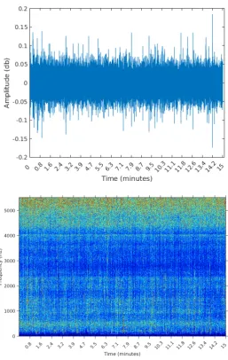
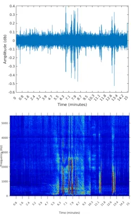
The third sample is from 2015-02-08, sunday, from 11h26m39s to 11h41m39s. During this 15 minutes there are many events taking place; listening to this sample we identify the engine of smaller vessels, being turned on and off and near the hydrophone spot. In this sample, we expect the segmentation algorithm to detect many events; by visually inspecting this sample, we identify 32 distinct segments.
Figure 8: Waveform and spectrogram of third sample: many short events
We apply our sequential segmentation algorithm to each of this samples; we take β ∈ {3×
10−5,1×10−5}and fixα= 0.01. Our experiments show that higher values forβresult in an excess of segments. For comparison we also apply Palshikar’s algorithm to the same samples, using theS1 function, withk= 11.025 fixed andh∈ {3,5}.
Because both our algorithm and Palshikar’s involve calculation of some function (the posterior distribution for ¯t, in our case, and the functionSifor Palshikar’s) for each coordinateytof the signal vector, when analysing samples as long as 15 minutes, with a sampling frequency of 11.025 Hz, the performance of both algorithms became unpractical (more than 10 minutes to process each sample). To deal with this situation, we adopt the strategy of fixing a time resolutionr= 11.025 to our algo-rithm, and a time resolution ofr= 10 to Palshikar’s. This means that we will calculate the posterior only foryj·11.025, j= 1, ..., f loor(N/11.025), and theS function foryj·10, j= 1, ..., f loor(N/10).
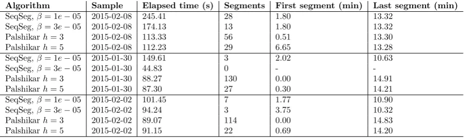
Algorithm Sample Elapsed time (s) Segments First segment (min) Last segment (min)
SeqSeg,β= 1e−05 2015-02-08 245.41 28 1.80 13.32
SeqSeg,β= 3e−05 2015-02-08 174.13 13 1.80 13.32
Palshikarh= 3 2015-02-08 113.33 56 0.51 13.30
Palshikarh= 5 2015-02-08 112.23 29 6.65 13.28
SeqSeg,β= 1e−05 2015-01-30 149.61 3 2.02 10.63
SeqSeg,β= 3e−05 2015-01-30 44.83 0 -
-Palshikarh= 3 2015-01-30 88.27 130 0.00 14.91
Palshikarh= 5 2015-01-30 87.30 27 0.30 14.21
SeqSeg,β= 1e−05 2015-02-02 101.45 7 1.77 10.90
SeqSeg,β= 3e−05 2015-02-02 94.24 3 3.75 10.32
Palshikarh= 3 2015-02-02 89.07 114 0.00 14.83
Palshikarh= 5 2015-02-02 91.15 22 0.69 14.20
Table 2: Results in real signal samples; see text for details
Table 2 summarizes the results of both algorithms applied to each of the three samples. We present the elapsed time, in seconds, the final number of segments, and the start time in minutes of the first and last segments.
The sample from 2015-01-30 is the sample containing only noise. We then expect the algorithms to output 0 segments. This was the case only for the SeqSeg algorithm whenβ= 3e−05. Palshikar’s algorithm returned many false positives for this sample, regardless of the parameter value.
The sample from 2015-02-02 is the sample containing a long event, starting at the very beginning of the file (0 minutes) and ending around 10 minutes. Again, the SeqSeg algorithm found a much lower number of segments and correctly identified the end of the main event at around 10 minutes.
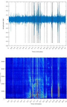
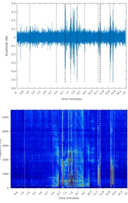
Finally, the sample from 2015-02-08 contains 32 segments evident to the eye. The SeqSeg algo-rithm came near to this number whenβ = 1e−05. It is noteworthy that, regardless of the value of β, the first and last segments found by SeqSeg had precisely the same starting points (this will always be the case, since calculation of the change points is completely deterministic). Palshikar’s algorithm came near to the true value of segments whenh= 5, and was less robust in terms of the starting times of the first and last segments.
Figure 12: Segmentation using Palshikar’s algorithm withh= 5
It is clear that the segments defined by the SeqSeg algorithm are much closer to what we can visually identify as meaningful events. The peak detection algorithm tends to oversegment the eventful sections, and ignore some points where there is a clear change in the signal’s power.
Finally, when applying both algorithms to real data, the computational performance of the two methods where not very different. We recall, however, that we imposed a resolution limitation to the SeqSeg algorithm. Nevertheless, even with this limitation, its results are clearly superior to the traditional peak detection strategy.
6
Conclusions
Our goal in this paper was to define a signal segmentation algorithm that could be as general as possible. We wanted it to be general specially because we do not know in advance exactly what kinds of patterns (events) there might be in the data. In this sense, this algorithm can be described as an unsupervised learning method, and could be applied to the analysis of any signal or time series where the assumptions hold.
The value of this parameter can be set by a technician with no mathematical training, by choosing an adequate sample to use for tuning the algorithm’s behavior.
Also, our method was built based on a simple assumption (that a segment involves a change in the signal’s energy), and based entirely on methods of Bayesian inference. There is no adhockeries involved, the closest to anad hocprocedure being the choice of the prior distributions. However, we have argued for the choice of each of the priors, and we believe that all of them honestly reflect and incorporate the prior knowledge that we have about the signal and the segments.
Most (if not all) automatic segmentation algorithms currently known to the literature, on the contrary, rely on more or less arbitrary definitions and parameters (such as the form of theSfunctions or the parameter h). We believe that, for this reason, the calibration of such algorithms is much more difficult than in our method, and our tests show that this is indeed the case.
On the other hand, the computational performance of our method is far from ideal. We acknowl-edge that and are currently working on a new and parallelized version of the algorithm, that we hope will perform significantly better.
There are also other ways to improve the performance of our algorithm, the simplest way being in using smaller sample sizes and for the MCMC algorihm. Experiments show that the main results are unaltered if we use samples of size 5000 instead of 10000. Also, there are other methods to obtain samples from a posterior distribution, in particular the Approximate Bayes Computation techniques [Chiachio (2014)] [Beck (2014)] [Beck (2014B)] [Chiachio (2017)], that might help reducing the com-putation time, specially in the FBST step. We are currently investigating these possibilities.
We believe, however, and since our algorithm is aimed at being used as a preprocessing tool, that the current performance is tolerable in the face of the quality of our results.
This work was partly supported by FAPESP grants 16/02175-0 and CNPq grant 308405/2013-7. The authors are grateful for the support received from IME-USP, the Institute of Mathematics and Statistics of the University of Sao Paulo; FAPESP - the State of S˜ao Paulo Research Foundation (grants CEPID-CeMEAI 2013/07375-0 and CEPID-Shell-RCGI 2014/50279-4); and CNPq - the Brazilian National Counsel of Technological and Scientific Development (grant PQ 301206/2011-2).The authors acknowledge the Laje de Santos Marine State Park Team for supporting this project. The authors would like to acknowledge professors Carlos Pereira and Victor Fossaluza for very helpful insights in this research project. In particular, they were the ones first suggesting that we should follow a general approach before trying to model specific events. Finally, the author would like to thank three anonymous referees for very helpful comments on the first draft of this paper.
References
[Bretthorst (1988)] Brethorst, L.Bayesian Spectrum Analysis and Parameter Estimation, Springer-Verlag: New York, USA, 1988; ISBN 978-0-387-96871-1
[Jaynes (1987)] Jaynes, E. Bayesian Spectrum and Chirp Analysis, In Maximum-Entropy and Bayesian Spectral Analysis and Estimation Problems, C.R. Smith, G.J. Erickson, Eds.; D. Reidel Publishing Co., Dordrecht, Holland, 1987; ISBN 978-94-009-3961-5
[Ruanaidh (1996)] Ruanaidh, J.J.K., Fitzgerald, W.J.Numerical Bayesian Methods Applied to Sig-nal Processing, Springer, New York, USA, 1996; ISBN 978-0387946290
[Bretthorst (1990A)] Bretthorst, L. Bayesian Analysis. I. Parameter Estimation Using Quadrature NMR Models,Journal of Magnetic Resonance1990,88, 533-551
[Bretthorst (1990B)] Bretthorst, L. Bayesian Analysis. II. Signal Detection and Model Selection, Journal of Magnetic Resonance199088, 552-570
[Bretthorst (1990C)] Bretthorst, L. Bayesian Analysis. III. Applications to NMR Signal Detection, Model Selection and Parameter Estimation,Journal of Magnetic Resonance1990,88, 571-595
[Etter (2013)] Etter, P.C.Underwater Acoustic Modeling and Simulation, CRC Press, Boca Raton, USA, 2013; ISBN 978-1-4665-6494-7
[Hubert (2017)] Hubert, P., Padovese, L.R., Stern, J.M. Full bayesian approach for signal detection with an application to boat detection on underwater soundscape data, to appear inMaximum Entropy Methods in Science and Engineering, Springer-Verlag, New York, USA
[Makowsky (2014)] Makowsky, R., Hossa, R. Automatic Speech Signal Segmentation Based on the Innovation Adaptive Filter,Int. J. Appl. Math. Comput. Sci2014,24 (2), 259-270
[Schwartzman (2011)] Schwartzman, A., Gavrilov, Y., Adler, R.J. Multiple Testing of Local Maxima for Detection of Peaks in 1D,The Annals of Statistics2011,39 (6), 3290-3319
[Kuntamalla (2014)] Kuntamalla, S., Ram Gopal Reddy, L. An Efficient and Automatic Systolic Peak Detection Algorithm for Photoplethysmographic Signals,International Journal of Com-puter Applications2014,97 (19)
[Theodorou (2014)] Thedorou, T., Mporas, I., Fakotakis, N. An Overview of Automatic Audio Seg-mentation,I.J. Information Technology and Computer Science2014,11, 1-9
[Jaynes (1982)] Jaynes, E.T. On the Rationale of Maximum-Entropy Methods, Proceedings of the IEEE1982,70 (9)939-952
[Jaynes (1968)] Jaynes, E.T. Prior Probabilities, IEEE Transactions On Systems Science and Cy-bernetics1968,4 (3)227-241
[Jeffreys (1946)] Jeffreys, H. An Invariant Form for the Prior Probability in Estimation Problems, Proceedings of the Royal Society of London. Series A, Mathematical and Physical Sciences 1946.186 (1007), 453-461
[Good (1992)] Good, I.J. The Bayes/Non-bayes compromise: a Brief Review,Journal of the Amer-ican Statistical Association1992,87 (419)597-606
[Perez (2014)] Perez, M., Pericchi, L.R. Changing Statistical Significance with the Amount of Infor-mation: The AdaptativeαSignificance Level,Statistics & Probability Letters2014,85, 20-24 DOI: 10.1016/j.spl.2013.10.018
[Pereira (1993)] Pereira, C.A.B., Wechsler, S. On the Concept of P-value, Revista Brasileira de Probabilidade e Estatistica1993,7159-177
[Pereira (1999)] Pereira, C.A.B., Stern, J.M. Evidence and credibility: full Bayesian significance test for precise hypotheses,Entropy1999,199-110
[Chakrabarty (2017)] Chakrabarty, D. A New Bayesian Test to Test for the Intractability-Countering Hypothesis,JASA2017,112 (518), 561-577
[Hubert (2009)] Hubert, P., Lauretto, M., Stern, J.M. FBST for Generalized Poisson Distributions AIP Conference Proceedings2009,1193 (1)210-217 DOI: 10.1063/1.3275617
[Lauretto (2009)] Lauretto, M.S., Nakano, F., Faria Jr., S.R., Pereira, C.A.B., Stern, J.M. A straight-forward multiallelic significance test for the Hardy-Weinberg equilibrium law, Genetics and Molecular Biology2009,32 (3)http://dx.doi.org/10.1590/S1415-47572009000300028
[Stern (2002)] Stern, J.M., Zacks, S. Testing the independence of Poisson variates under the Holgate bivariate distribution: the power of a new evidence test,Statistics & Probability Letters2002, 60 (3), 313-320
[Palshikar (2009)] Palshikar, G.K. Simple Algorithms for Peak Detection in Time Series, In1st Int. Conf. Advanced Data Analysis, Business Analytics and Intelligence2009
[Chiachio (2014)] Chiachio, M., Beck., J.M., Chiachio, J., Rus, G. Approximate Bayesian Compu-tation by Subset Simulation,SIAM Journal of Scientific Computing2014
[Beck (2014)] Beck, J.L., Zuev, K.M. Asymptotically independent Markov Sampling: A new MCMC scheme for Bayesian inference,Second International Conference on Vulnerability and Risk Anal-ysis and Management (ICVRAM) and the Sixth International Symposium on Uncertainty, Modeling, and Analysis (ISUMA)https://doi.org/10.1061/9780784413609.203
[Beck (2014B)] Beck, J.L., Taflanidis, A. Prior and Posterior Robust Stochastic Predictions for Dy-namical Systems Using Probability Logic,Int. Journal of Uncertainty Quantification2014