On linking the filter width to the boundary layer thickness
in explicitly filtered large eddy simulations of
wall bounded flows
by
Md. Mahfuz Sarwar
Centre for Environmental Safety and Risk Engineering (CESARE)
College of Engineering and Science
Victoria University
Submitted in total fulfilment of the requirements of
the degree of Doctor of Philosophy
ii
Declarations
“I, Md. Mahfuz Sarwar, declare that the PhD thesis entitled ‘On linking the filter width to the
boundary layer thickness in explicitly filtered large eddy simulations of wall bounded flows’ is
no more than 100,000 words in length including quotes and exclusive of tables, figures,
appendices, bibliography, references and footnotes. This thesis contains no material that has been
submitted previously, in whole or in part, for the award of any other academic degree or diploma. Except where otherwise indicated, this thesis is my own work”.
iii
Abstract
Computational fluid dynamics (CFD)-based three-dimensional predictive fire models are
increasingly used for predicting fire growth and spread. The models provide information to fire
safety engineers for designing fire protection systems in buildings. Although currently limited, in
a generation CFD-based models are expected to be used by emergency organisations to obtain
similar information during bushfires under a wide range of topographies, climates and types of
vegetation for their resource allocation planning. To increase their accuracy, most promising
CFD-based models are embedded with pyrolysis sub-models along with large eddy simulation
(LES) schemes to account for turbulence. The fundamental idea of LES is to resolve the large
energy containing eddies, and use sub-grid scale (SGS) model to simulate the effect of energy
dissipation by small scale eddies on large eddies.
Obtaining grid independent LES can be elusive. The filtering technique, along with the SGS
model, plays an important role in grid sensitivity and accuracy of LES. It is known that grid
sensitive simulations present a major problem with implicitly filtered LES and this can lead to
poor grid convergence. In the last two decades, explicit filtering schemes have appeared as a
viable option offer a promising solution, where the model (essentially the filter width) is
maintained constant while the discretization error is reduced by refining the grid. Implicit filter
tend not to separate discretization error from the modelling error because they do not separate the
turbulence model from the grid refinement. This leads to grid sensitive results even at low
Reynolds number for wall bounded flows. A growing body of literature is available in which it is
argued that explicit schemes are more likely to provide grid independent solutions and reduce the
iv for wall bounded flows is proposed to obtain grid independence by combining an explicit LES
scheme with a damped Smagorinsky sub-grid model. The aim is to separate modelling error from
numerical error and thereby to obtain a grid independent result more readily. In this approach,
emphasis is given to the selection of the filter width as a function of a physical parameter,
namely boundary layer thickness (BLT). An analysis of the energy spectrum ensures that grid
converged solutions at fixed filter are consistent with LES principles by setting fixed filter width
within the inertial sub-range and accurately capturing all energy containing eddies.
In this study, an open source implicitly filtered LES code, Fire Dynamics Simulator (FDS), is
taken as the baseline source code. First, the elusiveness of the grid convergence with the baseline
four implicitly filtered LES sub-models (standard Smagorinsky, dynamic Smagorinsky,
Deardorff and Vremen) is demonstrated. Out of the four, standard Smagorinsky model is found
to be most promising for a high Reynolds number (𝑅𝑒) flow. Then, this LES sub-model is
modified to implement the explicitly filtered LES. This modified model and approach is
successfully applied to two benchmark cases at two different two different 𝑅𝑒𝜆. A low 𝑅𝑒𝜆 case
is realized in a buoyancy driven turbulent flow in a differentially heated cavity, and a high 𝑅𝑒𝜆
flow occurs over a backward facing step. The proposed approach provides a possible alternative
way of selecting the LES filter in the absence of DNS resolutions as references. This study
provides guidelines on the selection of filter width to grid spacing ratio (ultimately BLT to grid
spacing ratio) for the proposed numerical scheme for resolving turbulent flows. This study also
shows that the performance of explicit LES with coarser resolution is better than the implicit
v
Acknowledgements
I would like to thank my supervisors, Associate Professor Khalid Moinuddin and Professor
Graham Thorpe from Victoria University, and Dr Matthew Cleary from the University of
Sydney, for their active support, guidance, inspiration and encouragement.
I would also like to thank:
Drs Randall McDermott and Kevin McGrattan from NIST, USA, Dr Jason Floyd from Hughes
Associates, USA and Dr Ruddy Mell from the U.S. Forest Service for their active support in
providing the technical information required on the FDS fire model through the FDS and
Smokeview discussion group.
Dr Duncan Sutherland for his generous support, assistance and sharing of knowledge.
H. M. Iqbal Mahmud and Sk Md Kamal Uddin, post-graduate students at Victoria University and
my colleagues, for their active support, motivation and valuable advice throughout this
challenging research work.
The Director of Centre for Environmental Safety and Risk Engineering (CESARE), Professor
Vasily Novozilov for his kind support in the final phase of my degree.
Bushfire Cooperative Research Centre (BCRC), Australia for their financial assistance and
providing a scholarship, and Victoria University for waiving my tuition fees during the PhD
vi Syeda Lutfunnesa, my mother, Salma Sultana my sister, Sadek, Saeed, Mahmud, and Murad my
brothers, Syed Shahidul Haque my uncle, and other friends and family members for their
continuous support, motivation and inspiration during ups and downs of this long journey of
research.
Most importantly, above all, Nazia Nawshin, my wife for her endless support, inspiration,
cooperation and patience and my two beloved sons Rehan and Nashwan for their understanding
as well as their love and affection.
Md. Mahfuz Sarwar
vii
Dedication
viii
Table of Contents
Declarations ... ii
Abstract ... iii
Acknowledgements... v
Table of Contents ... viii
List of figures ... xii
List of tables ... xvi
Nomenclature ... xviii
1.
Chapter 1 ... 1
Background Theory and Scope ... 1
1.1 Introduction ... 1
1.2 Numerical approaches to simulating turbulent flows ... 2
1.2.1 Direct Numerical Simulation (DNS) ... 2
1.2.2 Reynolds Averaged Navier-Stokes Simulation (RANS) ... 5
1.2.3 Large Eddy Simulations (LES) ... 6
1.3 Contribution of filtering schemes in LES ... 12
1.3.1 Implicit LES schemes ... 14
1.3.2 Explicit LES schemes ... 15
1.3.2.1 Selection of filter width in explicit LES scheme ... 16
1.3.2.2 Filter to grid spacing ratio (FGR) in explicit schemes ... 18
1.4 Research gap and limitations ... 18
1.5 Aims and research objectives ... 20
2.
Chapter 2 ...23
Governing equations and numerical schemes ... 23
2. 1 Introduction ... 23
ix
2.2.1 Standard Smagorinsky model ... 25
2.2.2 Dynamic Smagorinsky model ... 33
2.2.3 Deardorff model ... 34
2.2.4 Vreman model ... 35
2.3 A systematic approach to explicit scheme ... 36
2.3.1 Overall concept ... 36
2.3.2 Proposed explicit filter width ... 38
2.3.3 Filter width to grid spacing ratio ... 39
2.4 Governing equations of explicit LES scheme ... 39
2.4.2 Sub-grid closure ... 42
2.4.3 Damping function for model coefficient ... 43
2.4.4 Filter functions ... 43
2.4.5 Energy equation ... 44
2.4.6 Pressure equation ... 45
2.5 Calculation of energy spectrum ... 45
2.6 Defining nature of studied flows ... 46
2.6.1 Estimation of Reynolds number ... 46
2.6.2 Estimation of Rayleigh numbers ... 46
2.7 Solution algorithm ... 47
2.7 Conclusions ... 50
3.
Chapter 3 ...51
Assessment of baseline code ... 51
3.1 Introduction ... 51
3.2 Numerical simulation ... 52
3.4 Results and discussions - grid sensitivity ... 56
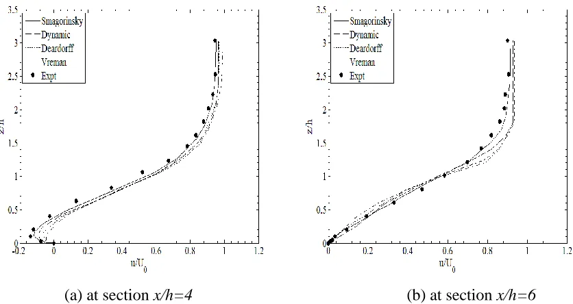
3.4.1 Graphical comparison -mean velocity and turbulence intensity ... 57
3.4.2 Quantitative comparison - mean velocity and turbulence intensity ... 59
3.5 Results and discussions - predicted outcomes ... 61
3.5.1 Statistical analysis of predicted outcomes ... 61
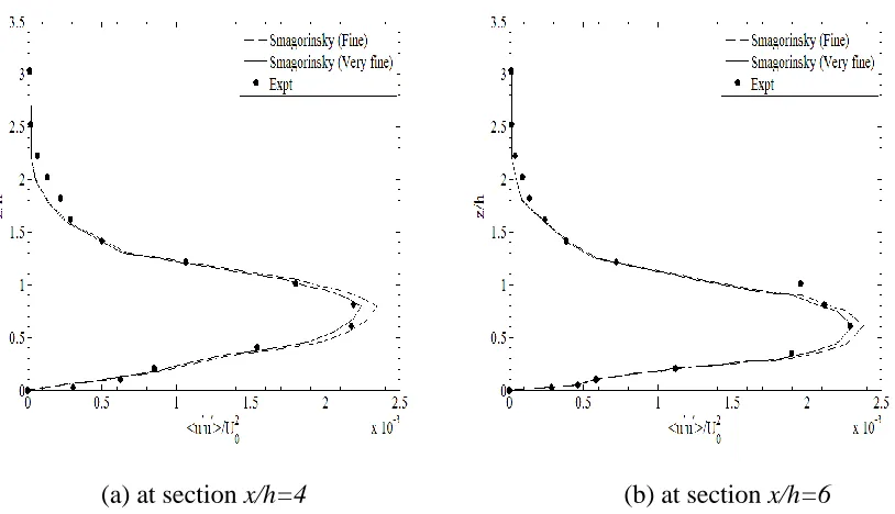
3.6 Further simulation with standard Smagorinsky model ... 65
3.7 Conclusions ... 68
x
High Reynolds number turbulent flow ... 69
4.1 Studied numerical configuration ... 69
4.2 Results and discussions ... 72
4.2.1 Energy spectra analysis ... 73
4.2.2 The congruence of energy spectra with flow variables ... 77
Mean velocity ... 77
Turbulence intensity ... 79
4.2.3 Validation of the proposed model ... 82
4.2.3.1 Graphical comparison ... 82
Mean velocity ... 82
Turbulence intensity ... 86
Summary of the validation exercise ... 88
4.2.3.2 Statistical analysis of predicted outcomes... 89
4.2.3.3 Comparison between simulation with implicit and explicit filtered LES ... 91
4.2.4 Prominent features of the flow ... 93
4.3 Conclusions ... 93
5.
Chapter 5 ...96
Low Reynolds number turbulent flow ... 96
5.1 Studied numerical configuration ... 96
5.2 Results and discussions ... 101
5.2.1 Energy spectra analysis ... 101
5.2.2 The congruence of energy spectra results with flow variables ... 107
Mean velocity ... 107
Non dimensional mean temperature ... 110
5.2.3 Validation of the proposed model ... 111
5.2.3.1 Graphical comparison ... 112
Mean velocity ... 113
Non dimensional mean temperature... 116
Summary of results validation ... 118
5.2.3.2 Statistical analysis of predicted outcomes... 118
5.2.4 Prominent flow features ... 120
xi
6.
Chapter 6 ...125
Conclusions and future work ... 125
6.1 Conclusions ... 125
6.2 Future work and recommendations ... 127
6.3 Applications ... 128
References ...129
Appendix A ...138
Details of Energy Spectra ... 138
Appendix B ...151
Simulation of Turbulent Pipe Flow ... 151
Appendix C ...160
xii
List of figures
Figure 1.1. Comparison of DNS, RANS and LES in terms of (a) computational costs and (b)
degree of modelling scales ... 6
Figure 1.2. Representation of resolved and sub-grid scales (SGS)in LES(Sagaut 2001) ... 7
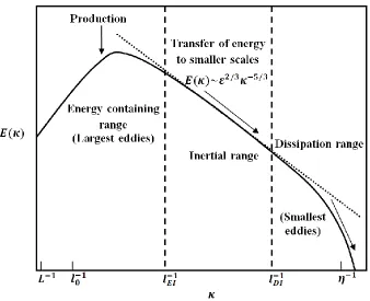
Figure 1.3. Energy cascading process from largest eddy scales to smallest eddy scales in terms of turbulent kinetic energy (vertical) and wavenumbers (inversely proportional to the length scales) plotted in log-log scales ... 13
Figure 2.1. Unfiltered and filtered turbulent field showing decomposition used in large eddy simulation ... 24
Figure 2.2. Simulation of energy cascading process in DNS, LES and RANS. Vertical dashed line (𝑙𝐸𝐼−1) demarcates the inertial and the energy containing range and the dashed line 𝑙𝐷𝐼−1 demarcates the inertial and the dissipation range ... 26
Figure 2.3. Energy spectrum decomposition process in RANS ... 27
Figure 2.4. Energy spectrum decomposition process in LES ... 28
Figure 2.5. Filtered energy spectra for box and Gaussian filters ... 29
Figure 2.6. Grid convergence of a hypothetical energy spectrum with progressively larger filter to grid ratios (FGR) Δ/δx1 < Δ/δx2 < Δ/δx3. The dashed vertical line indicates the cut-off wavenumber for the fixed filter width Δ ... 37
Figure 2.7. Hypothetical scenario of selection of filter width in an explicit scheme. Schematic shows the LES solution for four different filter widths with Δ1 > Δ2 > Δ3 > Δ4 (all grid converged) and vertical lines are corresponding cut-off wavenumbers. ... 38
Figure 3.1. Schematic view of backward facing step flow configuration (not to scale) ... 52
xiii
Figure 3.3. Mean velocity profiles at test section x/h=6 for the SGS models ... 56
Figure 3.4. Turbulence intensities at test section x/h=4 for the SGS models ... 57
Figure 3.5. Turbulence intensities at test section x/h=6 for the SGS models ... 58
Figure 3.6. Comparison of the mean velocity profile at test sections x/h=4 and x/h=6 for the SGS models ... 63
Figure 3.7. Comparison of the turbulence intensity profile at test sections x/h=4 and x/h=6 for the SGS models ... 64
Figure 3.8. Comparison of the mean velocity profile at test sections x/h=4 and x/h=6 for the standard Smagorinsky model for ℎ/𝛿𝑧 = 20 ... 65
Figure 3.9. Comparison of the turbulence intensity profile at test sections x/h=4 and x/h=6 for the standard Smagorinsky model for ℎ/𝛿𝑧 = 20 ... 66
Figure 4.1. Schematic diagram of grid used in Case 12 for a backward facing step ... 72
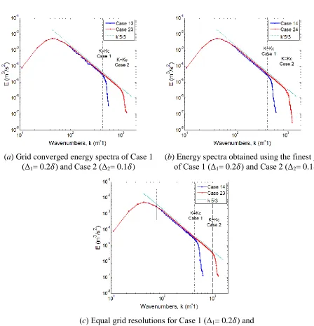
Figure 4.2. Grid-convergence of three-dimensional energy spectra for the high Reynolds number flow with two different fixed filter widths. ... 73
Figure 4.3. Energy spectra analysis for cases in which the grid size is maintained constant and the filter width is varied. Case 1 (Δ1= 0.2δ) and Case 2 (Δ2= 0.1δ) ... 75
Figure 4.4. Mean velocity at four test sections for fixed filter Case 1 (Δ1= 0.2δ) ... 78
Figure 4.5. Mean velocity profiles at four test sections for fixed filter Case 2 (Δ2= 0.1δ) ... 79
Figure 4.6. Turbulence intensities at selected test sections for fixed filter Case 1 (Δ1= 0.2δ) ... 80
Figure 4.7. Turbulence intensities at selected test sections for fixed filter Case 2 (Δ2= 0.1δ) ... 81
xiv
Figure 4.9. Mean velocity obtained with the finest grid resolution for fixed filter Case 1 (Δ1=
0.2δ) and Case 2 (Δ2= 0.1δ) ... 84
Figure 4.10. Mean velocity grid converged solution at same grid resolution for fixed filter Case 1 (Δ1= 0.2δ) and Case 2 (Δ2= 0.1δ) ... 85
Figure 4.11. Grid converged solution of turbulence intensities at relatively coarse grid resolution for fixed filter Case 1 (Δ1= 0.2δ) and Case 2 (Δ2= 0.1δ) ... 86
Figure 4.12. Turbulence intensities obtained with the finest grid resolution for fixed filter Case 1 (Δ1= 0.2δ) and Case 2 (Δ2= 0.1δ) ... 87
Figure 4.13. Grid converged solution of turbulence intensities at same grid resolution for fixed filter Case 1 (Δ1= 0.2δ) and Case 2 (Δ2= 0.1δ) ... 89
Figure 4.14. Instantaneous streamwise velocity at 12s along the midsection of the high Reynolds number flow over a backward facing step. Results are for Case 23 ... 93
Figure 5.1. Schematic of buoyancy driven flow inside a differentially heated rectangular cavity with particular emphasis is given to boundary layer development near the hot wall ... 97
Figure 5.2. Schematic diagram of grid resolutions for (a) Case 12 (b) Enlarged view near the top wall of rectangular cavity... 100
Figure 5.3. Grid-convergence of three-dimensional energy spectra for the low Reynolds number flow with two different fixed filter widths ... 102
Figure 5.4. Energy spectra analysis with various grid and fixed filter combination for Case 1 (Δ1= 0.2δ) and Case 2 (Δ2= 0.1δ) ... 103
Figure 5.5. The model spectra at various Reynolds numbers (Pope 2000) ... 105
Figure 5.6. Mean velocity at four test sections for fixed filter Case 1 (Δ1= 0.2δ) ... 107
xv
Figure 5.8. Mean temperatures at four test sections for fixed filter Case 1 (Δ1= 0.2δ) ... 109
Figure 5.9. Mean temperature at four test sections for fixed filter Case 2 (Δ2= 0.1δ) ... 110
Figure 5.10. Mean velocity grid converged solution at relatively coarser grid resolution for fixed filter Case 1 (Δ1= 0.2δ) and Case 2 (Δ2= 0.1δ) ... 112
Figure 5.11. Mean velocity obtained with the finest grid resolution for fixed filter Case 1 (Δ1=
0.2δ) and Case 2 (Δ2= 0.1δ) ... 113
Figure 5.12. Mean velocity grid converged solution at same grid resolution for fixed filter Case 1 (Δ1= 0.2δ) and Case 2 (Δ2= 0.1δ) ... 114
Figure 5.13. Mean temperature grid-converged solutions at relatively coarser grid resolutions for fixed filter Case 1 (Δ1= 0.2δ) and Case 2 (Δ2= 0.1δ) ... 115
Figure 5.14. Mean temperature obtained with the finest grid resolution for fixed filter Case 1 (Δ1= 0.2δ) and Case 2 (Δ2= 0.1δ) ... 116
Figure 5.15. Mean temperature grid converged solution at same grid resolution for fixed filter Case 1 (Δ1= 0.2δ) and Case 2 (Δ2= 0.1δ) ... 117
Figure 5.16. Snapshot of the shaded streamline plot (a) and vector plots (b) & (c) of velocity
inside the differentially heated cavity along the midsection at quasi-steady state after
approximately 150 s. Results are for Case 23 ... 121
Figure 5.17. A snapshot of the isotherms plots obtained after 2s of initiating the experiment, (b)
depicts the temperature distribution at the quasi steady state. (c) & (d) that also indicate the
quasi-steady state temperature and flow field on the mid-section of a differentially heated cavity.
xvi
List of tables
Table 2.1. Smagorinsky constant (Cs) for different types of filter ... 32
Table 3.1. Considered model coefficients and estimated wall unit (n+) values of SGS models .. 54
Table 3.2. Grid convergence measures (GCI) of the mean velocity profiles at stations x/h=4 and
x/h=6 for flow over a backward facing step ... 60
Table 3.3. Grid convergence measures (GCI) of the turbulence intensity at stations x/h= 4 and
x/h=6 for flow over a backward facing step ... 60
Table 3.4. Relative error analysis of the mean velocity profile (fine resolution) at stations x/h=4
and x/h=6 for flow over a backward facing step ... 62
Table 3.5. Relative error analysis of the turbulence intensity (fine resolution) at stations x/h= 4
and x/h=6 for flow over a backward facing step ... 62
Table 3.6. GCI of the mean velocity and the turbulence intensity profiles of standard
Smagorinsky model at stations x/h=4 and x/h=6 with very fine grid (h/δz=20)... 67
Table 3.7. Relative errors of the mean velocity and the turbulence intensity profiles of standard
Smagorinsky model at stations x/h=4 and x/h=6 with very fine grid (h/δz=20)... 67
Table 4.1. Selected filter sizes Δ1and Δ2 for a turbulent flow at high Reynolds numbers ... 70
Table 4.2. Grid resolutions for flow over a backward facing step at a high Reynolds number,
Reλ=115 ... 71
Table 4.3. Cross-stream averaged relative error of mean streamwise velocity in grid-converged
cases with different filter widths for flow over a backward facing step ... 90
Table 4.4. Cross-stream averaged relative error of streamwise velocity variance in
xvii Table 4.5. Comparison of relative error of streamwise velocity and velocity variance between
implicit and explicit filtered LES ... 92
Table 5.1. Filter sizes Δ1 and Δ2 for a turbulent flow at low Reynolds numbers ... 98
Table 5.2. Grid resolutions for a buoyancy driven differentially heated cavity flow at a low
Reynolds number, Reλ =25 ... 99
Table 5.3. Relative mean error analysis of mean velocity and dimensionless temperature for
Case 13 and Case 14 for cavity flow ... 119
Table 5.4. Relative mean error analysis of mean velocity and dimensionless temperature for
xviii
Nomenclature
𝐴 integration constant in energy spectrum
𝐴+ van Driest constant
𝐵 integration constant in velocity profile taken to be 5.2
𝐵𝛽 expansion of velocity field using Taylor series in Vreman’s model (m2/s2)
𝐶 Kolmogorov constant
𝑐 Vreman’s eddy model coefficient (𝑐 = 2.5𝐶𝑆)
𝐶𝜇 turbulent viscosity constant in the standard 𝑘 − 𝜀 model
𝐶𝜀1, 𝐶𝜀2 model constants in the standard 𝑘 − 𝜀 model
𝐶𝑆 Standard Smagorinsky model coefficient
𝐶𝑆_𝐷𝑎𝑚𝑝 Smagorinsky coefficient (𝐶𝑆) using the Van Driest damping function
𝐶𝑖𝑗 cross-stresses (N/m2)
𝐶𝑣 Deardorff model coefficient
𝐸(𝜅) energy spectrum(m3/s2)
𝐸̂ (𝜅) filtered energy spectrum(m3/s2)
𝐸𝑓 filtered kinetic energy from the filtered velocity field (m3/s2)
𝑒𝑖𝑗 dissipation tensor (m2/s3)
𝐹𝑖 external force (N/m2)
𝐹𝐾𝑙𝑒𝑏 Klebanoff intermittency function
𝑓𝑙(𝜅𝑙) function of wavenumbers based on integral lengthscale
xix
𝐺(𝑟) filter function in LES
𝐺̂(𝜅) filter transfer function in LES
𝐺𝑟𝑥 Grashofs number
𝑔 acceleration due to gravity (9.81 m/s2)
𝐻(𝑥) Heaviside function
𝐻 cavity height (m)
𝜅 von Karman constant
𝜅 wavenumbers (m−1)
𝜅𝐸𝐼 demarcation wave number between energy containing(𝜅 > 𝜅𝐸𝐼) and inertial
range (𝜅 < 𝜅𝐸𝐼) (m−1)
𝜅𝐷𝐼 demarcation wave number between inertial (𝜅 > 𝜅𝐷𝐼) and dissipation range
(𝜅 < 𝜅𝐷𝐼) (m−1)
𝑘 turbulent kinetic energy (m2/s2 )
𝑘𝑠𝑔𝑠 turbulent kinetic energy of SGS model (m2/s2 )
𝑘𝑟 turbulent kinetic energy for the residual part in LES (m2/s2 )
𝐿 width of cavity (m)
𝑙 characteristic length scale (m)
𝑙0 integral length scale (m)
𝑙𝐸𝐼 demarcation between energy containing(𝑙 > 𝑙𝐸𝐼) and inertial range (𝑙 < 𝑙𝐸𝐼)
𝑙𝐷𝐼 demarcation between inertial (𝑙 > 𝑙𝐷𝐼) and dissipation range (𝑙 < 𝑙𝐷𝐼)
𝑙𝑚𝑖𝑥 mixing length (m)
xx
𝑀𝑖𝑗 model parameter in dynamic Smagorinsky model
𝑁𝑥, 𝑁𝑦, 𝑁𝑧 number of grid points in three spatial directions
𝑃𝑟 production rate from the residual kinetic energy (m2/s2 )
𝑝 pressure (N/m2)
𝑝̅ mean pressure (N/m2)
𝑝′ fluctuating pressure (N/m2)
𝑝̂ filtered pressure (N/m2)
𝑅 radius or center line of the pipe (m)
𝑅𝑖𝑗 Reynolds stresses (N/m2)
𝑅𝑖𝑗(𝑟, 𝑥) two-points velocity correlations (m2/s2 )
𝑅𝑎 Rayleigh number
𝑅𝑒 Reynolds number
𝑅𝑒𝑥 Reynolds number based on the characteristic length 𝑥
𝑅𝑒𝜏 Reynolds number based on the frictional velocity
𝑅𝑒𝜆 Taylor scale Reynolds number
𝑅𝑒𝑙 Reynolds number based on the system or largest eddy length scale
𝑅𝑒𝜂 Reynolds number based on the Kolmogorov length scale
𝑆̅ filtered strain rate (s−1)
𝑆̅𝑖𝑗 filtered rate of stress tensor (s−1)
𝑆𝑖𝑗 rate of strain tensor (s−1)
𝑆̂ filtered strain rate in explicit scheme (s−1)
xxi
𝑇𝑠 surface temperature of cavity wall (K)
𝑇∞ ambient temperature (K)
𝑡0 time scale relates to integral length scale (s)
𝑡𝐸 eddy turnover time (𝑠)
𝑡𝜂 time scale relates to Kolmogorov length scale (s)
𝑈𝑒 boundary layer edge velocity (m/s) at various streamwise locations
𝑈(𝑥, 𝑡) turbulent flow field of velocity (m/s)
𝑢, 𝑣, 𝑤 Cartesian velocity components along three directions (3-D) (m/s)
𝑢 instantaneous velocity (m/s)
𝑢+ dimensionless wall normal velocity
𝑢(𝑙) characteristic velocity (m/s)
𝑢𝑚𝑎𝑥 maximum velocity at the center line (m/s)
𝑢0 velocity relates to integral length scale (m/s)
𝑈0 free stream velocity (m/s) at reference location (3h upstream of the step)
𝑢𝜂 velocity relates to Kolmogorov length scale (m/s)
𝑢𝜏 friction velocity (m/s)
𝑢̅, 𝑣̅, 𝑤̅ mean velocity component in three direction (m/s)
𝑢′, 𝑣′, 𝑤′ fluctuating velocity component along three direction (m/s)
𝑢′𝑣′
̅̅̅̅̅ Reynolds stresses (m2/s2 )
𝑢̅(𝑥, 𝑡) filtered resolved velocity component (m/s)
𝑢′(𝑥, 𝑡) residual (or SGS) velocity component (m/s)
xxii
〈𝑢̃𝑖〉 ensemble average of the filtered velocity (m/s)
𝑢̂ filtered velocity in LES (m/s)
𝑢′ fluctuating part of the velocity in LES (𝑢𝑅𝑒𝑠𝑜𝑙𝑣𝑒𝑑′ + 𝑢𝑅𝑒𝑠𝑖𝑑𝑢𝑎𝑙′ )(m/s)
𝑊𝑗 given weights to the cell within the filter width
𝑥 position (m)
𝑦 Cartesian coordinate
𝑦+ dimensionless wall normal unit
𝑦𝑐𝑟𝑜𝑠𝑠𝑜𝑣𝑒𝑟 smallest distance which separates two layers of the boundary layer (m)
Greek symbols
𝛼 test and grid filter width ratio (∆̂/∆)
𝛼 thermal diffusivity of fluid in cavity flow (m2/s)
𝛼 closure coefficient in Cebeci-Smith model considered as 0.0168
𝛼, 𝛽 arbitrary initial values in turbulent pipe flow
𝛼𝑖𝑗 velocity gradient in Vreman’s model
𝛽 thermal expansion coefficient in cavity flow (K−1)
𝛽, 𝑐𝜂 constants in model spectrum based on Taylor scale Reynolds number (𝑅𝑒𝜆)
𝛿 boundary layer thickness (m)
𝛿𝑥, 𝛿𝑦, 𝛿𝑧 grid (or mesh) cell size in three direction (3-D) (m)
𝛿𝑖𝑗 Kronecker delta
𝛿𝑣∗ velocity thickness (m)
Δ spatial filter width in LES (m)
xxiii
𝜀 dissipation of turbulent kinetic energy (TKE) (m2/s3)
𝜀𝑓 filtered dissipation energy (m2/s3)
𝜉 relative error at an individual point
𝜉𝑚 resultant mean relative error
Φij(κ) velocity spectrum (m2/s2)
ℒ𝑖𝑗 Leonard stress term known as ‘Germano identitity’ (N/m2)
𝜆 Taylor microscale (m)
𝜇 molecular viscosity of the fluid (kg/m. s)
𝜇𝑇 turbulent molecular viscosity of the fluid (kg/m. s)
𝜂 Kolmogorov length scale (m)
𝜈 kinematic viscosity of fluid (m2/s)
𝜈𝑇 turbulent kinematic viscosity of fluid (m2/s)
𝜈𝑚𝑖𝑥 kinematic viscosity of mixing length (m2/s)
𝜈𝑡𝑖𝑛𝑛𝑒𝑟 viscosity near the wall (m2/s)
𝜈𝑡𝑜𝑢𝑡𝑒𝑟 viscosity outer boundary layer (m2/s)
𝜌 density (kg/m3)
𝜎𝑘 turbulent Prandtl number for kinetic energy
𝜎𝜀 turbulent Prandtl number for dissipation
ℛ reference values
𝜓 predicted values from numerical solution
𝜏𝑖𝑗 shear stress tensor (N/m2)
xxiv
𝜏(𝑙) characteristic timescale (s)
𝜏𝜂 Kolmogorov timescale (s)
𝜏0 integral length scale timescale(s)
𝜏𝑤 wall shear stress (N/m2)
𝜏𝑖𝑗𝑠𝑔𝑠 sub grid scale shear stress (N/m2)
𝜏𝑖𝑗𝑅𝑒𝑠𝑜𝑙𝑣𝑒𝑑 resolved stress part of SGS model (N/m2)
𝜏𝑖𝑗𝑅𝑒𝑠𝑖𝑑𝑢𝑎𝑙 residual stress part of SGS model (N/m2)
Superscripts
〈. 〉 spatial averaging
Acronyms
𝐵𝐿𝑇 Boundary layer thickness
𝐶𝐹𝐷 Computational fluid dynamics
𝐷𝑁𝑆 Direct numerical simulation
𝐹𝐺𝑅 Filter to grid spacing ratio
𝐿𝐸𝑆 Large eddy simulation
𝑁𝑆 Navier-Stokes equations
𝑃𝐷𝐸 Partial differential equation
𝑅𝐴𝑁𝑆 Reynolds averaged Navier-Stokes simulation
𝑆𝐺𝑆 Sub-grid scale
𝑆𝑆𝑀 Standard Smagorinsky model
1
1.
Chapter 1
Background Theory and Scope
1.1 Introduction
It is vital that fire safety engineers are able to predict the growth and spread of building-fires
under a wide range of scenarios in order to design fire protection systems. It is also important for
emergency organisations to predict similar effects during bushfires under a wide range of
topographies, climates and types of vegetation for their resource allocation planning. Compuational fluid dynamics (CFD)-based three-dimensional predictive fire models are highly
desirable for both groups of professionals. While pyrolysis (gasification of solid fuel) and
combustion (chemical reaction between gasified fuel and oxygen) sub-models are distinguishing
features of a CFD-based fire model, its background sub-models of mass, momentum and energy
are fundamentally important.
Numerical simulation becomes more complex when a flow field becomes turbulent. Almost
every flow scenario of practical importance is turbulent in nature. Turbulent flow is characterized
by random fluid motions from small scale to large scale motions at various frequencies. Although the largest scale in fire scenarios can be ranged from tens of meters (building fires) to
many kilometers (bushfires), the phenomena that determine their behaviour and accuracy are
dependent on the scales that may be tiny fractions of a millimeter. To capture these tiny motions
the spatial and temporal resolutions in numerical simulation need to be extremely fine, which
requires enormous computational resources. A simulation scheme to solve mass, momentum and
2 reduce the computational requirements, various numerical schemes have emerged. They fall into
two broad categories, Reynolds averaged Navier-Stokes (RANS) simulation, and large eddy
simulation (LES). More details of the mathematical formulation of the governing equations and
numerical approaches to solving these governing equations in DNS, RANS and LES are
discussed in several sections of this chapter.
1.2 Numerical approaches to simulating turbulent flows
The main concept of numerical simulation of turbulent flow using CFD is that it approximates
fluid motions by solving a set of non-linear partial differential equations (PDEs). These
differential equations consist of continuity equations (mass conservation) and momentum
balance equations (Navier-Stokes equations) derived from Newton’s second law of motion. For
compressible flow, an additional energy equation is required to extract the necessary information
about the density and temperature (Pope 2000). In the momentum and energy equations,
convective non-linear terms appear which make them intractable to solve analytically.
In numerical approaches, these governing partial differential equations are discretized in space
and time in the computational domain of a given physical problem using different types of
numerical schemes. As mentioned above, there are three broad numerical approaches for solving
Navier-Stokes equations: DNS, RANS and LES.
1.2.1 Direct Numerical Simulation (DNS)
DNS solves the Navier-Stokes equations by resolving all the spatial and temporal scales of
turbulence present in the flow, and this results in particularly accurate solutions. The continuity
and the Navier-Stokes equations for incompressible flow are as follows:
𝜕𝑢 𝜕𝑥+
𝜕𝑣 𝜕𝑦+
𝜕𝑤 𝜕𝑧 = 0
3 𝜌 (𝜕𝑢 𝜕𝑡 + 𝑢 𝜕𝑢 𝜕𝑥+ 𝑣 𝜕𝑢 𝜕𝑦+ 𝑤 𝜕𝑢 𝜕𝑧) = 𝐹𝑥− 𝜕𝑝 𝜕𝑥+ 𝜇 (
𝜕2𝑢
𝜕𝑥2+
𝜕2𝑢
𝜕𝑦2+
𝜕2𝑢
𝜕𝑧2)
(1.2) 𝜌 (𝜕𝑣 𝜕𝑡 + 𝑢 𝜕𝑣 𝜕𝑥+ 𝑣 𝜕𝑣 𝜕𝑦+ 𝑤 𝜕𝑣 𝜕𝑧) = 𝐹𝑦− 𝜕𝑝 𝜕𝑦+ 𝜇 (
𝜕2𝑣
𝜕𝑥2 +
𝜕2𝑣
𝜕𝑦2 +
𝜕2𝑣
𝜕𝑧2)
(1.3) 𝜌 (𝜕𝑤 𝜕𝑡 + 𝑢 𝜕𝑤 𝜕𝑥 + 𝑣 𝜕𝑤 𝜕𝑦 + 𝑤 𝜕𝑤 𝜕𝑧) = 𝐹𝑧− 𝜕𝑝 𝜕𝑧+ 𝜇 (
𝜕2𝑤
𝜕𝑥2 +
𝜕2𝑤
𝜕𝑦2 +
𝜕2𝑤
𝜕𝑧2)
(1.4)
Here, 𝑢, 𝑣 and 𝑤are the velocity components along three directions; 𝐹 is the external force, 𝑝 is
the pressure and 𝜇 represents the molecular viscosity of the fluid. In tensor form, these governing
equations can be simply expressed as
𝜕𝑢𝑖 𝜕𝑥𝑖 = 0
(1.5) 𝜌 (𝜕𝑢𝑖 𝜕𝑡 + 𝑢𝑗 𝜕𝑢𝑗 𝜕𝑥𝑗) = 𝐹𝑖 − 𝜕𝑝 𝜕𝑥𝑖 + 𝜇 (
𝜕2𝑢 𝑖
𝜕𝑥𝑗𝜕𝑥𝑗)
(1.6)
In DNS, neither turbulence modelling of effects of small scales on large scales nor the averaging
approach to obtain mean and fluctuating components is involved. Since it is the most accurate
numerical approach to capture the turbulence, in many cases it is considered as an alternative to
physical experimentation. For instance, where experimental results are not available, the DNS
results are considered as the most accurate numerically obtained solutions for validating the
results from numerical simulations with turbulence modelling.
The major issue that affects the practical use of DNS results is the higher computational
requirements. In DNS the grid spacing must be on the same lengthscale as the smallest eddies.
Hence, details of turbulent flows that occur in many practical situations can be captured only by
using a very large number of grid points. This is computationally resource intensive. In addition,
the required grid resolutions depend on the Reynolds number (𝑅𝑒) which is a dimensionless
4
When the 𝑅𝑒 increases, the ratio between the integral lengthscale and smallest lengthscale also
increases (Pope 2000) (for more details about scales please refer to Section A.3 of Appendix A).
To date the largest DNS performed of an idealised channel flow are of order 𝑅𝑒𝜏 ~ 5200 (Lee
and Moser 2015).
In DNS, all of the smallest scales that are responsible for energy dissipation are captured. In
those cases, the computational grid size should be small enough to capture these viscous effects
of flow. The grid size should be smaller than the size of the smallest eddies and this ranges from
less than a millimetre (George 2005) in all practically important flows; the smallest length scale
present in turbulent flows is known as the Kolmogorov scale, 𝜂. If we consider 𝐿 as the
characteristic length of the computational domain, so for DNS, the number of grid points in one
direction will be in the order of,
𝑁~𝐿 𝜂
(1.7)
The Kolmogorov lengthscale is represented in terms of the kinematic viscosity 𝜈 (𝑚2/𝑠) and
dissipation (the rate at which turbulent kinetic energy is converted into internal energy) per unit
mass of the fluid 𝜀(𝑚2/𝑠3). Therefore 𝜂 is represented as; 𝜂 = (𝜈3/𝜀)1/4. The dissipation per
unit mass can be approximated as 𝜀~𝑢3/𝐿, where 𝑢 is the characteristic velocity of the flow.
Using these relations, the number of grid points in a domain required for DNS can be estimated
as,
𝑁~ (𝐿 𝜂)
3
~ (𝑢𝐿 𝜈 )
9/4
= 𝑅𝑒9/4 (1.8)
For this reason, DNS is not computationally feasible for high Reynolds numbers and is restricted
to relatively low Reynolds numbers and is mostly used for comparatively simple fluid flow cases
5 practical cases and complex engineering applications, DNS will not be able to provide numerical
solutions by using high performance computational power that is presently available. For
example, in atmospheric applications the 𝑅𝑒 is of order 𝑅𝑒𝜏~ 2.5 × 10⁶ and the geometries can
be quite complex such as flow over buildings (Bou-Zied et. al 2009).
1.2.2 Reynolds Averaged Navier-Stokes Simulation (RANS)
The Reynolds averaged Navies-Stokes simulation (RANS) is one of the most widely used
numerical approaches to simulate turbulent flows. It takes the time averaged solution of
Navier-Stokes equations to solve the fluid flow. This idea was first introduced by Reynolds (1895). The
underlying concept behind RANS is the Reynolds decomposition which separates instantaneous
fluid motions into two components, namely time averaged mean values and fluctuating
quantities. The auto-correlation of fluctuating components are termed as ‘Reynolds stresses’
which are modelled using empirically determined relationships. The time averaged
Navier-Stokes equations in all three spatial directions can be written as,
𝜌 (𝜕𝑢̅ 𝜕𝑡 + 𝑢̅ 𝜕𝑢̅ 𝜕𝑥+ 𝑣̅ 𝜕𝑢̅ 𝜕𝑦+ 𝑤̅ 𝜕𝑢̅ 𝜕𝑧) = 𝐹𝑥− 𝜕𝑝̅ 𝜕𝑥+ 𝜇 (
𝜕2𝑢̅
𝜕𝑥2+
𝜕2𝑢̅
𝜕𝑦2+
𝜕2𝑢̅
𝜕𝑧2) − 𝜌 (
𝜕𝑢̅̅̅̅̅′𝑢′
𝜕𝑥 +
𝜕𝑢̅̅̅̅̅′𝑣′
𝜕𝑦 +
𝜕𝑢̅̅̅̅̅′𝑤′
𝜕𝑧 ) (1.9)
𝜌 (𝜕𝑣̅ 𝜕𝑡 + 𝑢̅ 𝜕𝑣̅ 𝜕𝑥+ 𝑣̅ 𝜕𝑣̅ 𝜕𝑦+ 𝑤̅ 𝜕𝑣̅ 𝜕𝑧) = 𝐹𝑦− 𝜕𝑝̅ 𝜕𝑦+ 𝜇 (
𝜕2𝑣̅
𝜕𝑥2+
𝜕2𝑣̅
𝜕𝑦2+
𝜕2𝑣̅
𝜕𝑧2) − 𝜌 (
𝜕𝑢′𝑣′̅̅̅̅̅
𝜕𝑥 +
𝜕𝑣′𝑣′̅̅̅̅̅
𝜕𝑦 +
𝜕𝑣′𝑤′̅̅̅̅̅̅
𝜕𝑧 ) (1.10)
𝜌 (𝜕𝑤̅ 𝜕𝑡 + 𝑢̅ 𝜕𝑤̅ 𝜕𝑥 + 𝑣̅ 𝜕𝑤̅ 𝜕𝑦+ 𝑤̅ 𝜕𝑤̅ 𝜕𝑧) = 𝐹𝑧− 𝜕𝑝̅ 𝜕𝑧+ 𝜇 (
𝜕2𝑤̅
𝜕𝑥2+
𝜕2𝑤̅
𝜕𝑦2+
𝜕2𝑤̅
𝜕𝑧2) − 𝜌 (
𝜕𝑢′𝑤′̅̅̅̅̅̅
𝜕𝑥 +
𝜕𝑣′𝑤′̅̅̅̅̅̅
𝜕𝑦 +
𝜕𝑤′𝑤′̅̅̅̅̅̅
𝜕𝑧 ) (1.11)
In tensor form, thee equations can be expressed as
𝜕𝑢̅𝑖 𝜕𝑡 + 𝑢̅𝑗 𝜕𝑢̅𝑗 𝜕𝑥𝑗 = 𝐹𝑖− 1 𝜌 𝜕𝑝̅ 𝜕𝑥𝑖+ 𝜈
𝜕2𝑢̅ 𝑖 𝜕𝑥𝑗𝜕𝑥𝑗− 𝜕𝑢𝑖′𝑢 𝑗′ ̅̅̅̅̅̅ 𝜕𝑥𝑗 ⏟ 𝑅𝑒𝑦𝑛𝑜𝑙𝑑𝑠 𝑆𝑡𝑒𝑠𝑠𝑒𝑠 (1.12)
where 𝜈 represents the kinematic viscosity; 𝜈 = 𝜇/𝜌.
The process of averaging inevitably results in loses of information. As a result, RANS models
lose detailed information of the flow, more specifically the details of the flow smeared as it
6 1.2.3 Large Eddy Simulations (LES)
In LES, turbulence contained in large lengthscales is resolved and small scale turbulence is
modelled. Comparing computational costs, LES lies between DNS and RANS. The levels of
turbulence modelling employed in three numerical approaches in terms of computational cost are
shown in Figure 1.1. DNS captures all turbulence down to small scales, and provides fully
resolved solutions which increases the computational time and cost and has been shown in
Figure 1.1 (a). On the other hand, RANS takes the shortest time for the simulation compared to
LES and DNS, but is unable to give detailed information on turbulence. However, LES lies
between DNS and RANS in terms of computational cost and time illustrated in Figure 1.1 (b).
LES is capable of simulating complex flows and geometries such as flow over bluff bodies
where flow separation and rotation both take place (You et. al. 2007).
(a) (b)
Figure 1.1. Comparison of DNS, RANS and LES in terms of (a) computational costs and (b) degree of modelling scales
As capturing small scales is computationally very expensive, in LES, large scale eddies are
resolved over a number of computational cells and small scale eddies are filtered by filter width
which is generally of the same as the grid size. Figure 1.2 represents how LES separates large
and small eddies in physical space by using a filtering technique through the filter width (∆). It
7 as grid size here) are resolved and the dissipative motions of small eddies are filtered. Effects of
dissipative motion of eddies (which are smaller than the filter size) on energy containing large
eddies are modelled by sub-grid scaling which saves computation time and cost compared to
DNS. The resolved length scales are directly captured by the numerical scheme. On the other
hand, various turbulence models (e.g. Smagorinsky model, dynamic models etc.) account for the
effect that the unresolved scales has on the resolved scales. These models are also known as
sub-grid scale (SGS) models (Gullbrand 2004).
Figure 1.2. Representation of resolved and sub-grid scales (SGS)in LES (Sagaut 2001) The filtering process plays an important role in LES. Generally, LES can be characterised by two
types of filtering: implicit (where filter width is same as the grid size) and explicit (where filter
width is explicitly set by the modeller). However, implicit LES has a significant implication; it
directly depends on the grid size. If the grid changes the model changes with grid which results
in different solutions. Moreover, it has less control over the discretization errors (Mahesh et. al.
2006, Youet. al. 2007). Thus, grid convergence becomes elusive using implicit LES. Unless grid
converged solutions are obtained the results of CFD simulations are of uncertain value.
Subgrid-scale (SGS) models in LES
Over the last two decades SGS models in LES have advanced significantly for complex
8 models (referred to as coarse DNS) generate unphysical results due to the accumulation of
energy at the high wavenumbers. Therefore, an appropriate SGS model ensures the fidelity of
LES.
The concept of SGS models was first introduced in meteorological simulations. Smagorinsky
(1963) proposed an eddy viscosity model to simulate atmospheric boundary layer turbulence
which was based on the Boussinesq hypothesis or approximation. This model captured the
principal effects of the SGS stresses in flows. It relates turbulent shear stress to the mean flow
strain rate. In some cases it is termed as gradient transport (Tennekes and Lumley 1972, Libby
1996).
𝑢′𝑣′ ̅̅̅̅̅~1
2( 𝜕𝑢̅ 𝜕𝑦+
𝜕𝑣̅
𝜕𝑥) (1.13)
This approximation is suggested in analogous to Newton’s law of viscosity with the statement that ‘shear stress is proportional to strain rate’, where viscosity is the proportionality constant.
𝜏 = 𝜇 (𝜕𝑢
𝜕𝑥) (1.14)
where 𝜏 is the local shear stress. The important fact is that this statement holds for laminar flow
and is well supported by experimental results. Turbulent flow generates additional mixing of
momentum and turbulent shear stress can be expressed as
−𝑢′𝑣′̅̅̅̅̅ = 𝜈𝑇(𝜕𝑢̅ 𝜕𝑦+
𝜕𝑣̅
𝜕𝑥) (1.15)
where, 𝜈𝑇 is the turbulent viscosity. From this expression it appears that the Boussinesq
hypothesis relates the comparatively small scale statistical behaviour known as Reynolds stress
to large scale behaviour (statistical information extracted from mean flow behaviour).
Smagorinsky used an analogous idea to develop an eddy viscosity subgid-scale model based on
this Boussinesq approximation which relates subgrid-scale stresses to the eddy viscosity. It is
9 constant) was derived by Lilly (1966) for homogeneous and isotropic turbulence. Performance of
the Smagorinsky model was first explored by Deardorff (1970) for three-dimensional channel
flow driven by a uniform pressure gradient at high Reynolds number (𝑅𝑒𝐻 ≈ 240,000 based
upon the channel height). From the study, he concluded that the agreement between the
computed statistics and the experimental data of Laufer (1954) was in poor agreement and the
accuracy of the numerical approach was expected to be improved with an increase of numerical
resolution.
One of the challenges associated with LES is to model the effects of small scale eddies and to
derive governing equations inclusive of them. To address the modelling problem, Leonard
(1974) proposed the derivation of LES governing equations using the filtering concept. The
concept of filter kernel is to separate small and large scale eddies by applying a spatial filter to
the velocity field. A volume averaged filter was formulated by Schumann (1975) and applied to
the simulation of incompressible turbulent channel flows. In his proposed model, SGS stresses
are divided into two parts, one is accounting for isotropic turbulence and the other for anisotropic
effects of turbulence. Schumann concluded that the results with the SGS model were in good
agreement with the channel flow experimental data. The concept of spectral eddy viscosity was
presented by Kraichnan (1976) and applied to isotropic turbulence. Using this model, he showed
the limitations of the eddy viscosity concept to represent the effects of small scale turbulence. The extension of Kraichnan’s work was carried out by Leslie and Quarini (1979) where they
presented a theoretical formulation of SGS modelling procedures. From this study, they supported Kraichnan’s findings that the effective eddy viscosity varies with the wavenumbers
associated with different eddy lengthscales. They tested the SGS model for isotropic flow and
10 tensor formulations for periodic homogeneous isotropic turbulence at low Reynolds number.
They restricted their study to Reynolds number (based on the Taylor microscale) in the range of
𝑅𝑒𝜆 ≤ 40 due to lack of computational capacity. Simulation results showed that large scale
eddies were well captured by energy spectrum analysis but the performance of the SGS model
was only moderately good. The idea of scale-similarity was first introduced by Bardina et al.
(1980). This idea helps to express the sub-grid field quantities in terms of filtered quantities. The
study indicates that information in the resolved scales is sufficient to describe some
characteristics of the fluid flow and the argument 'production equals dissipation' does not
applicable to small scale turbulence decay. Another feature of this model is that it produces
backscatter (energy transfer from small scale to large scale eddies) of energy. However, from
simulations it is found that the model does not dissipate enough energy which leads to inaccurate
results. This problem was addressed by Germano et al. (1991), and they proposed a dynamic
SGS modelling approach where a model coefficient is not prescribed but it is computed
dynamically. LES with the proposed dynamic SGS model was used to simulate a fully developed
turbulent channel flow. Germano et al. (1991) found the results were in good agreement with the
DNS results of Kim et al. (1987). However, the mathematical formulation of dynamic SGS
model has some inconsistencies and it is restricted to flows that are statistically homogenous in
at least one direction, a fact identified by Goshal and Moin (1995). They rectified the
inconsistency of the mathematical formulation of Germano’s work and studied filter
inhomogeneity for isotropic turbulence and found the obtained results are in good agreement
with experiments. Goshal (1996) addressed the issues of discretization error (generated from
finite differencing) and aliasing errors (generated from non-linear terms in SGS) in LES using a
11 (cutoff or discard negative model coefficients) negative values and to minimise the singularities
in dynamic modelling, Meneveau et al. (1996) proposed a dynamic SGS model in which SGS
stresses are formulated in Lagrangian way by using first-order Euler time integration and linear
interpolation in space. The constant and dynamic Smagorinsky models and their variations are
most widely used SGS models. The interested reader can refer to the books of Sagaut (2001),
Pope (2000) and Wilcox (1993) for an extensive review of SGS models used in LES.
Numerical methods in LES
Numerical methods play an important role in ensuring the accuracy of simulations. Numerical
schemes that are used for LES often rely on finite-difference methods or spectral methods as
they are computationally less expensive than finite element and finite volume methods (Goshal
1996). LES is prone to numerical errors that arise from discretization and aliasing, that are
directly dependent on the numerical schemes.
Goshal (1996) studied numerical errors in LES for various finite difference methods (from 2nd
order to 8th order) and spectral methods. He found that higher order schemes lead to reduction in
the numerical errors. Kravchenko and Moin (1997) studied the effects of numerical errors in LES
by performing numerical simulation of turbulent channel flow using finite difference methods
and spectral methods. Numerical and analytical studies show that aliasing errors are more
destructive for spectral and fourth and sixth-order difference than for second-order
finite-difference simulations. They assumed the probable reason is aliasing errors (generated from the
non-linear terms with finite differencing) may cause numerical instability and excessive
turbulence decay for both spectral and higher-order numerical schemes compared to lower-order
numerical scheme for the test case. Further investigations of Goshal (1996) were carried out by
Moin and Chow (2003) where they gave emphasis to numerical as well as modelling errors that
12 method. Findings of their study are consistent with those of Goshal (1996) that higher order
numerical schemes have more control over numerical errors. Gullbrand and Chow (2003)
presented the effects of numerical errors of second and fourth order finite difference schemes to
assess the performance of implicitly and explicitly filtered LES (discussed in Section 1.3.1 and
1.3.2, respectively) for various SGS models. They observed the difference between the
simulation results and reference data for different SGS models was larger for the fourth order
than for the second order code. They assumed this may be due to the coarser resolution used in
the fourth-order code compared to the resolution of the second-order code. Kempf et al. (2011)
studied numerical error of the turbulent non-premixed bluff-body flame using the Smagorinsky
model in LES, where the error is defined with respect to experimental data. From their study they
suggested that second-order scheme can be used in anisotropic turbulence in complex geometries
to obtain reasonable LES solutions. Keskinen et al. (2016) carried out numerical investigations
using four different SGS approaches for a three-dimensional, turbulent pipe flow (𝑅𝑒𝜏 = 360).
SGS models are the standard Smagorinsky, linear interpolation (non-dissipative), the Gamma
limiter (dissipative), and the scale-selective discretization (slightly dissipative). In their study,
they have used a second-order numerical scheme for the SGS models they considered. Out of
four SGS models, the authors found that that Smagorinsky model shows the best agreement with
the reference data.
1.3 Contribution of filtering schemes in LES
According to the classical theory of Kolmogorov, lengthscales of eddies in turbulent flows can
be divided into three regions (Pope 2000). It is considered that the largest eddies are the same
13 Figure 1.3. Energy cascading process from largest eddy scales to smallest eddy scales in terms of turbulent kinetic energy (vertical) and wavenumbers (inversely proportional to the length scales)
plotted in log-log scales
the fluid properties. This part in the energy spectrum of turbulence is known as the energy
containing range. Kolmogorov lengthscales are the smallest eddy scales. In these scales the
influence of viscosity is dominant and energy is transferred to surroundings by dissipation in the
form of heat: the local Reynolds number (Reynolds numbers calculated on the basis of eddy
length scales) is of the order of unity. Between these largest and smallest scales, other scales of
eddy exist and these eddy length scales can be expressed by comparatively large local Reynolds
numbers: they are independent of viscous effects. This intermediate class is known as inertial
subrange scales; they depend on the dissipation rate only and are fully independent of the types
of flow (whether wall bounded or free shear flow).
The intermediate and smallest eddy length scales are universal and they show an isotropic nature
14 in terms of wavenumbers (related to wavelength or eddy length scales and inversely proportional
to the characteristic lengthscale of an eddy) and the specific kinetic energy spectrum plotted on
logarithmic axes. This process of transferring energy from large eddies to smaller eddies is
known as an energy cascading process. It illustrates how energy is transferred between eddies
over a wide range of lengthscales. It was first introduced by Richardson (1922). Energy is
produced in the largest scale(𝑙0) eddies and is transferred via the inertial range to the
Kolmogorov scale (𝜂) where it is dissipated in the form of heat. The dissipation range is highly
influenced by viscous effects and occurs in the smallest scales. Whereas 𝑙𝐸𝐼 and 𝑙𝐷𝐼 presents the
demarcation between the energy containing and dissipation range from the inertial subrange
during the energy cascading process. According to Kolmogorov, the energy transferred from the
large energy containing range to the inertial range is equal to the energy transferred from the
inertial range to the dissipation range or Kolmogorov scales and further into heat (Pope 2000).
Advantage of this energy cascading property is taken in LES of turbulent flows where the effects
of the smallest scales on the largest scales are modelled as turbulent dissipation (Sagaut 2001).
Extended studies of LES and their most important aspects to resolve turbulence in many practical
and complex situations are discussed in the later sections of this chapter.
1.3.1 Implicit LES schemes
A large number of authors showed that implicit schemes are highly grid sensitive and fail to
control numerical errors (more specifically discretization errors). Higher order numerical
schemes in implicit LES were studied by Lund and Kaltenbench (1995) for turbulent flow inside
a pipe. They observed grid sensitivity even with a high order numerical scheme applied to
implicitly filtered LES. Sensitivity of implicitly filtered LES to the numerical grid due to the
15 Kravchenko and Moin (2000) in their numerical studies of flow over a circular cylinder at a low
Reynolds number (𝑅𝑒𝐷) 3900. They used both the dynamic and the standard Smagorinsky model
to conduct the implicitly filtered LES simulations. After comparing their results with
experimental data, they concluded that grid converged solutions are difficult to obtain by using
implicit LES even at very low Reynolds number fluid flow. Meyers & Sagaut (2007) conducted
a numerical study of channel flow at low Reynolds numbers (𝑅𝑒𝜏 = 298) using implicitly
filtered LES, and compared their results with DNS. After evaluating the performance of a
number of SGS models, they concluded that grid sensitivity remained, even when the grid was
very finely resolved.
1.3.2 Explicit LES schemes
Implicitly filtered LES can certainly converge to the limit of a DNS resolution, but it will in
general not converge to that limit monotonically thus complicating convergence analysis as the
literature reference above demonstrates. In the last two decades, explicit filtering schemes have
been investigated by various researchers in which the filter width is maintained constant thus
keeping the model unchanged while the numerical error is reduced by refining the grid (Carati et
al. 2001; Winckelmans et al. 2001). Explicitly filtered LES converges monotonically allowing
for a systematic approach to testing the grid sensitivity of the solutions (Matthew et al. 2003).
Ghosal and Moin (1995) and Ghosal (1996) discuss the advantages of explicit filtering over
implicit filtering in LES for isotropic turbulence inside a cubic configuration with periodic
boundary conditions. Najjar and Tafti (1996) simulated turbulent channel flow using an explicit
scheme. In their study, the focus was on the control of numerical errors that are generated due to
using explicit LES. They used different test filters (top hat and Fourier cut-off filters) in a
16 spacing obtained from DNS resolution of a channel flow study conducted by Kim et al. (1987).
Simulated results were compared with DNS where explicit LES was observed to provide more
accurate solutions than implicit LES.
Gullbrand (2002) studied grid independent LES for turbulent channel flow using explicit
filtering. She concluded that an explicit filter is able to provide grid independent results for
turbulent channel flow and to significantly reduce the numerical errors which are associated with
high wavenumbers generated from the convective term of the Navier-Stokes equations. The case
study was further expanded by Gullbrand and Chow (2003) to assess the errors associated with
different numerical schemes as well as SGS turbulence closures. They provided guidelines on
filter width to grid spacing ratio (FGR) for a number of numerical schemes. It was found that for
fourth-order finite difference schemes, an explicit filter width should be at least twice that of the
grid cell, and for second-order schemes it should be at least four times. These findings are
consistent with those of Chow and Moin (2003). More recently, Radhakrishnan and Bellan
(2012, 2013, 2015) have extensively studied grid independence of explicitly filtered LES for
single- and two-phase compressible fluid flows with evaporation inside an internal combustion
chamber. Prior to conducting grid independence tests, a DNS solution database was created which the authors termed a ‘trusted template’ for validating the LES results. A DNS study was
carried out because it was not possible to conduct experiments of the proposed test cases due to
complex boundary conditions.
1.3.2.1 Selection of filter width in explicit LES scheme
The selection of the filter width in explicit LES schemes has often been either inadequately
addressed, or in some cases completely ignored by previous researchers. Some authors do,
17 approach which means that a grid-converged LES solution is obtained by refining the grid while
the filter width (taken from a DNS study) is unchanged. From her study, it appears that she took
the filter width as being eight times the DNS grid resolution (∆= 8𝜕𝑥𝐷𝑁𝑆) although the rationale
for this is unclear. There were two computational grid resolutions selected for the simulation:
one was taken as 𝜕𝑥𝑐𝑜𝑎𝑟𝑠𝑒 = 4𝜕𝑥𝐷𝑁𝑆 corresponding to an FGR of two, and the second was
𝜕𝑥𝑓𝑖𝑛𝑒 = 2𝜕𝑥𝐷𝑁𝑆 corresponding to an FGR of four. A similar case study was performed by Gullbrand and Chow (2003) to assess the effect of numerical errors arising from different
numerical schemes. They ran implicit LES simulations with four coarse grid resolutions:
6𝜕𝑥𝐷𝑁𝑆, 4𝜕𝑥𝐷𝑁𝑆, 3𝜕𝑥𝐷𝑁𝑆 and 2𝜕𝑥𝐷𝑁𝑆 finding that 3𝜕𝑥𝐷𝑁𝑆 was the coarsest resolution that gave
the same results as those given by DNS with the grid size resolved to the Kolmogorov length
scale, and it was selected as the grid size required for explicit LES. However, based on the
assumption that a fourth-order numerical scheme would be more accurate than the second-order
scheme, a coarser grid, i.e. 4𝜕𝑥𝐷𝑁𝑆 was selected for the simulation in which a fourth order
scheme was implemented, whereas for the second order scheme it was maintained at 3𝜕𝑥𝐷𝑁𝑆. In
the cases of both numerical schemes they kept the filter width fixed at (8𝜕𝑥𝐷𝑁𝑆), leading to an
FGR of two, and nearly three for the fourth- and second-order schemes, respectively.
Radhakrishnan and Bellan (2012, 2013, 2015) followed a very similar approach in selecting the
filter width in explicit LES schemes. They selected three different meshes (coarse, 𝜕𝑥𝑐𝑜𝑎𝑟𝑠𝑒 =
4𝜕𝑥𝐷𝑁𝑆 with an FGR of two, medium, 𝜕𝑥𝑚𝑒𝑑𝑖𝑢𝑚 = 2𝜕𝑥𝐷𝑁𝑆, with an FGR of four and fine,
𝜕𝑥𝑓𝑖𝑛𝑒 = 𝜕𝑥𝐷𝑁𝑆, with an FGR of eight). For higher order numerical schemes the filter width was
taken as 8 times that of the DNS grid resolution. The literature indicates that a similar approach
has been adapted in almost every explicit scheme test case where filter widths are selected from
18 1.3.2.2 Filter to grid spacing ratio (FGR) in explicit schemes
Filter to grid spacing ratio (FGR) plays an important role in providing appropriate solutions in
explicit LES schemes. This issue has been reported by several authors by performing various
fluid flows using explicit schemes. Ghosal (1996) reported that significant numerical errors were
generated when performing explicit LES for isotropic turbulence decay inside a cubic box. The
author focused on the errors that were generated due to spatial discretization arising from finite
differencing schemes of different orders. One of the notable findings of his study was that a
significant portion of the numerical errors arose from the non-linear and sub-grid terms in LES.
According to their approximation the aliasing errors (errors from non-linear terms) are
independent of finite difference schemes. An extension of the work of Goshal (1996) was carried
out by Chow and Moin (2003). They investigated the numerical errors for a similar case study
using both low order (second order) and higher order (fourth and sixth order) explicit LES codes.
Their suggestions were that for a second-order finite difference scheme, the desired filter-grid
ratio is at least four and for a higher order (i.e. fourth or sixth order) numerical scheme an
filter-grid ratio of two is sufficient. Turbulent channel flow using explicit filtering was investigated by
Gullbrand and Chow (2003) to assess the effect of numerical errors for second- and fourth-order
numerical schemes. Furthermore, the case study was also investigated for various turbulence
models and grid resolutions. In this work, for fourth-order finite difference schemes the explicit
filter width an filter-grid ratio of two was found to be sufficient; for the second order it was four,
which supported the findings of Chow and Moin (2003).
1.4 Research gap and limitations
From the above survey of the literature, it is found that almost all the case studies with explicit
19 over a circular cylinder, etc.) and have not been used in any practical cases or in engineering
applications (Lee and Moser 2015). For simple flow cases, well-developed DNS reference data
are either available or can be generated without much difficulty. Therefore, it was
straightforward to choose the grids and/or filter width (explicit scheme) for LES, based on the
available/required DNS grid resolutions. Furthermore, there are no guidelines available to select
the filter width for other complex fluid flow cases where no reference resolutions (DNS) are
available. DNS cannot be easily performed to determine the filter width for explicit LES for
practical cases. An important question in the absence of DNS resolution is how to select the filter
width which is a purely model parameter in explicitly filtered LES. Can it be based on a
percentage of a physical parameter such as the boundary layer thickness (BLT), which is
considered the same size as the largest eddy (Tennekes and Lumley 1972)? It then raises the
second question: how can we select the percentage of a physical parameter and select an FGR
consistent with the principles of LES and grid convergence? The main objective of this current
work is to address the above issues and to develop an appropriate scheme to obtain a simulation
result consistent with the principles of LES which are (a) the filter width lies within inertial range
and (b) all energy containing eddies are adequately captured and grid convergence is obtained in
explicit schemes (Pope 2004).
The CFD-based model fire dynamics simulator (FDS) is a promising model for simulating
turbulent flows, arising from fire, with a reasonable degree of accuracy when the flow field is
highly resolved (Abubakar 2015). FDS is a time-dependent, three-dimensional computational
fluid dynamics CFD-based fire model used to solve the Navier-Stokes equations for turbulent
flows. It is an open source LES code developed by McGrattan et al.(2011). In this study, FDS