Journal of Fluid Mechanics
http://journals.cambridge.org/FLMAdditional services for
Journal of Fluid Mechanics:
Email alerts: Click here Subscriptions: Click here Commercial reprints: Click here Terms of use : Click here
Adjustment of a turbulent boundary layer to a canopy of
roughness elements
S. E. BELCHER, N. JERRAM and J. C. R. HUNT
Journal of Fluid Mechanics / Volume 488 / July 2003, pp 369 398 DOI: 10.1017/S0022112003005019, Published online: 02 July 2003
Link to this article: http://journals.cambridge.org/abstract_S0022112003005019 How to cite this article:
S. E. BELCHER, N. JERRAM and J. C. R. HUNT (2003). Adjustment of a turbulent boundary layer to a canopy of roughness elements. Journal of Fluid Mechanics, 488, pp 369398 doi:10.1017/ S0022112003005019
Request Permissions : Click here
DOI: 10.1017/S0022112003005019 Printed in the United Kingdom
369
Adjustment of a turbulent boundary layer to
a canopy of roughness elements
By S. E. B E L C H E R1, N. J E R R A M†2A N D J. C. R. H U N T3 1Department of Meteorology, PO Box 243, University of Reading, Reading, RG6 6BB, UK
2Department of Applied Mathematics and Theoretical Physics, University of Cambridge, Centre for
Mathematical Sciences, Wilberforce Road, Cambridge, CB3 0WA, UK
3Department of Space and Climate Physics, University College, Gower Street, London, UK
(Received22 May 2002 and in revised form 14 March 2003)
A model is developed for the adjustment of the spatially averaged time-mean flow of a deep turbulent boundary layer over small roughness elements to a canopy of larger three-dimensional roughness elements. Scaling arguments identify three stages of the adjustment. First, the drag and the finite volumes of the canopy elements decelerate air parcels; the associated pressure gradient decelerates the flow within an impact region
upwind of the canopy. Secondly, within an adjustment region of length of order Lc
downwind of the leading edge of the canopy, the flow within the canopy decelerates substantially until it comes into a local balance between downward transport of momentum by turbulent stresses and removal of momentum by the drag of the canopy elements. The adjustment length, Lc, is proportional to (i) the reciprocal of
the roughness density (defined to be the frontal area of canopy elements per unit floor area) and (ii) the drag coefficient of individual canopy elements. Further downstream, within a roughness-change region, the canopy is shown to affect the flow above as if it were a change in roughness length, leading to the development of an internal boundary layer. A quantitative model for the adjustment of the flow is developed by calculating analytically small perturbations to a logarithmic turbulent velocity profile induced by the drag due to a sparse canopy withL/Lc1, whereLis the length of
the canopy. These linearized solutions are then evaluated numerically with a nonlinear correction to account for the drag varying with the velocity. A further correction is derived to account for the finite volume of the canopy elements. The calculations are shown to agree with experimental measurements in a fine-scale vegetation canopy, when the drag is more important than the finite volume effects, and a canopy of coarse-scale cuboids, when the finite volume effects are of comparable importance to the drag in the impact region. An expression is derived showing how the effective roughness length of the canopy, zeff0 , is related to the drag in the canopy. The value of zeff0 varies smoothly with fetch through the adjustment region from the roughness length of the upstream surface to the equilibrium roughness length of the canopy. Hence, the analysis shows how to resolve the unphysical flow singularities obtained with previous models of flow over sudden changes in surface roughness.
1. Introduction
The surfaces of the Earth and oceans are covered with roughness elements, such as grass or bushes over land, or ripples and waves on the ocean. When the roughness
elements are small, it is conventional to consider only the flow over the roughness elements. However, when the roughness elements are larger, such as crops or buildings, it is often necessary to know details of the flow between the roughness elements as well as the flow over the group of roughness elements. It is then appropriate to think of the group of roughness elements as a canopy. Despite progress in the past few years in the use of the roughness length to parameterize effects of varying surface roughness, better modelling is needed, particularly for the non-uniform region in the vicinity of the roughness change, in order to tackle practical problems such as mesoscale numerical weather prediction and air quality forecasting in urban areas and hilly terrain, which then determine climatic and agricultural effects of air movements and fluxes in and out of these canopies.
The overall effects of a canopy of roughness elements on the turbulent flow that passes over them are usually parameterized as a roughness length, zeff0 . Such a parameterization is compact and effective in many applications, but has limitations. First, this method gives no information about the flow between the roughness elements themselves, which is required for modelling scalar transport in applications of urban air quality and dispersion in agricultural crops. Secondly, there is at present no general systematic method for obtaining the roughness length from the geometry of the roughness elements and their spatial distribution. Indeed, Grimmond & Oke (1999) have shown that the methods in current use cannot even explain satisfactorarily the flow over symmetrically distributed roughness elements of the same size, let alone those over typical non-uniform non-symmetrically distributed obstacles found in practice. Thirdly, the roughness length is only defined when the wind profile above the roughness elements is logarithmic. Hence, when the flow above the area of roughness elements is accelerating or decelerating it is not even clear whether or not the roughness length can be defined (Krettenauer & Schumann 1992). Finally, representing a change in the density or type of surface roughness elements by a change in their roughness lengths, z0, leads to unrealistically large changes in shear
stress at the upwind edge of a change (e.g. Belcher, Xu & Hunt 1990). The object of this paper is to develop understanding and quantitative modelling of these complex boundary-layer flows, and to suggest how to improve the use of the roughness length as a practical parameterization.
These problems are addressed here with a more refined treatment of the effects of the roughness elements on the flow. The calculations are based on the approximations, first, that the volume occupied by the canopy acts as a region of drag on the wind (see for example Kaimal & Finnigan 1995, chapter 3) and, secondly, that the finite volumes of the roughness elements of the canopy displace the flow. As noted by Finnigan (2000), previous work has focused on the conditions when the boundary layer is fully adjusted to the canopy, such as over large areas of vegetation. Here, since we are motivated particularly by winds over and within urban areas whose building densities are often inhomogeneous, we focus specifically on the adjustment of the boundary-layer flow as it approaches and passes over the canopy elements.
x L
z
U(z)
u*, z0
y
ge he LA
be
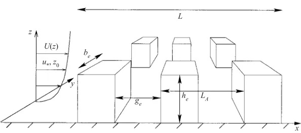
Figure 1. Geometry of the canopy elements and the approach flow.
the shear layer that forms at the top of the canopy (Hunt & Durbin 1999), and interaction between the boundary layer and canopy flows through eddies generated by a mixing-layer instability at the top of the canopy (Raupach, Finnigan & Brunet 1996). A third question, therefore, is whether a simple mixing length parameterization may be valid over part of the flow, as found in studies of flow over roughness changes (Belcheret al.1990) and studies of the mean wind profile within a vegetation canopy (Wilson, Finnigan & Raupach 1998). Fourthly, as in flow over roughness changes (Townsend 1976) and two-phase flows (Koweet al. 1988), the effects of the obstacles on the flow are modelled in an averaged sense over an area or volume occupied by many obstacles and by introducing an extra shear stress or body force into the momentum equations, rather than calculating the flow around each obstacle. Can these factors be defined in terms of simple properties of the roughness elements and the surface? These questions are addressed in this paper.
In§2, a model for boundary-layer flow through groups of obstacles is formulated by representing the obstacles as a canopy with a drag on the wind. In§2.1, a simple method is developed to estimate the mean drag exerted by the canopy on the mean flow in terms of properties of the canopy elements, with an analysis of the characteristic scales of flow and the flow perturbations in a homogeneous canopy. Depending on the density of the canopy, two different models for turbulent momentum transport within the canopy are developed in §2.2. The characteristics and scalings for how the boundary layer adjusts to the canopy are described in§3. The method of solving the resulting equations is described in §4. Comparisons of the model with previous computations and with measurements made both in the field and in the wind tunnel are shown in§5. Section 6 describes the variation of the effective roughness length of the canopy with distance through the canopy. Conclusions are given in §7.
2. Development of idealized models
A fully developed atmospheric boundary layer, with wind components U0 =
(U0(z),0,0), blows in the positive x-direction, with the z-axis pointing upwards
vertically, see figure 1. Here, we consider the changes to this boundary layer as it impinges upon a canopy, composed of a group of many solid roughness elements. To fix ideas, think of a canopy that extends over a lengthLand formed byNe elements,
with typical heighthe, breadthbe, and gap between canopy elementsge.
decelerates the mean flow. Secondly, the displacement of streamlines around individual canopy elements can also transports momentum. The aim here is to calculate the main effect of the canopy of obstacles by computing the spatially averaged time-mean flow, called here the mean flow. In this way, we compute the evolution of the flow as the canopy density varies, but avoid calculating the details of the flow around individual canopy elements. The spatial average is taken over a horizontal area with side of lengthLA. For a periodic array of obstacles,LAis the length of the repeating unit. For
a random array,LAencompasses several obstacles, such thatLAis much greater than
the gap between individual obstacles but much less than the length scale over which the mean obstacle density changes. This approach was initiated by Taylor (1944), see Batchelor (1967, §5.15), and has been further developed for flows in vegetation canopies, see Finnigan (2000).
Consider, for simplicity, the case when the fraction of the canopy volume occupied by obstacles, β, is small, i.e. the gap between the elements ge is large compared
with their breadth be, β∼b2e/g2e1. The aerodynamic drag of the obstacles, which
remains substantial, can then be represented by a point force at the centre of each roughness element. The spatial averaging operation renders these point forces into a continuous resistive body force that extends throughout the canopy volume. In addition, the displacement of streamlines by individual canopy elements yields, on averaging spatially, a net momentum transport, the dispersive stress described by Raupach & Shaw (1982) and Finnigan (1985). There is experimental evidence (Finnigan 1985; Cheng & Castro 2002a) that near the top of the canopy the dispersive stress is very small compared to the Reynolds stress. The dispersive stress may be a larger fraction near the bottom of the canopy (Bohm, Finnigan & Raupach 2000), but both stresses tend to be small there. Hence, as we shall see, the drag term is important through the whole volume of the canopy, whereas the dispersive stress can be neglected; although we shall see that the finite volumes of the canopy elements lead to a dispersive stress that is important upwind of the canopy.
We begin by analysing the effect of the drag term on the flow. Hence, on ignoring the dispersive stress, the equations governing the spatially averaged time-mean flow are
Uj ∂Ui ∂xj
+ ∂P ∂xi
= ∂τij ∂xj
−fi, (2.1)
∂Ui ∂xi
= 0. (2.2)
Hereinafter, xi = (x, y, z) and τ13 = τ, and the pressure, stress and drag force
are defined such that the density is one throughout. The model is completed on parameterizing the spatially averaged turbulent stress,τij, and drag per unit volume, fi. These aspects are considered next.
2.1. Relating the obstacle drag to the flow
First, the drag per unit volume, fi, is related to the spatially averaged time-mean
flow speed,U(x, y, z). Since the Reynolds number of the flow around the test element is large, the drag varies as the square of the impinging wind speed (Batchelor 1967, §5.11). The drag on the test element then scales asU2 and is reduced by the presence
of the other canopy elements (cf. Wood & Mason 1993). These arguments suggest that the drag on each canopy element scales on U2 multiplied by a factor that is independent of U. The spatial averaging smoothes these point forces to yield fi, the
drag per unit volume of canopy. Hence, on dimensional grounds,fi can be expressed
as the ratio of U2 and acanopy-drag length scale,Lc, namely
fi(x) = |U|Ui
Lc
, (2.3)
with Lcindependent ofU. The drag fi = 0 outside the canopy.
Explicit estimates for Lc are now obtained for illustration by considering an array
ofNe tall slender canopy elements, each with breadthbe and frontal areaAf ∼hebe,
and covering a total floor area At. At height z, the sectional drag coefficient, cd(z), is
defined, following MacDonald (2000), to be the drag at height z divided by half the square of the spatially averaged time-mean wind at that height, U2(z)/2, multiplied
by the frontal width (per unit floor area) presented to the flow by the obstacles, i.e. Nebe/At. The force per unit volume acting at heightz is then (Nebe/At)cd(z)U2(z)/2.
When the obstacles have a uniform horizontal cross-section, the height and breadth can be related to the frontal area throughbe=Af/ he. MacDonald (2000) shows how
this expression is related to a conventional (depth integrated) expression for the drag and drag coefficient.
Now, this drag of the canopy decelerates the fluid within the canopy and hence acts only within the fraction of volume occupied by fluid, (1−β). Hence, the drag is divided by a factor of (1−β). As β increases, this process becomes more important and is considered by Eames, Hunt & Belcher (2003). Taken together, for this illustrative case, there is an average force per unit volume acting on the fluid within the canopy ofU2N
e¯cdAf/2(1−β)heAt (where ¯cd is the average sectional drag coefficient), so that
the average canopy-drag length scale Lcis given by
1 Lc
= Ne
1 2¯cdAf
(1−β)heAt
=
1 2¯cdλ
(1−β)he
∼be/g2e, (2.4)
whereλ=NeAf/At ∼hebe/g2e is theroughness density(see also Wooding, Bradley &
Marshall 1973; Raupach 1992). We note that the coefficientNeAf/ heAt is equivalent
to the leaf area index,a, with units of m−1, referred to in the literature on forests and
plant canopies (e.g. Kaimal & Finnigan 1995, p. 79).
The model just developed is sufficiently flexible to account for inhomogeneous canopies. When the characteristics of the canopy elements vary in space, as they do through an urban area, the canopy length scale, Lc, also varies. Formally, this
variation must be on length scales greater than the averaging length scaleLA.
2.2. Models for the turbulent stress
Hunt et al. (2001) show that the dynamics of turbulence are approximately local,
so that the turbulent stress is approximated by Prandtl’s mixing-length model, when (i) the distortion time scale Td at which the mean shear and strain change along
the trajectories of fluid elements is comparable with or larger than the Lagrangian timescale of the energy containing eddies and (ii) the integral length scale Lx of
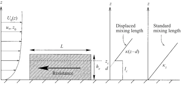
U0(z)
u*, z0
he
Resistance
L
z z
Standard mixing length Displaced
mixing length
zc
d lc jz
(z – d)
z
Figure 2. Geometry of the canopy and two models for the mixing-length.
canopy and generates mixing-layer-type eddies (Raupach et al. 1986), which satisfy these conditions only marginally. Hence, for homogeneous canopies, the mixing-length model has limitations (Raupachet al. 1996). Nevertheless, for the perturbed canopy flows considered here, the mixing-length model can be justified as the first term in an expansion (Finnigan & Belcher 2003). Hence, we adopt the mixing-length model here.
In the boundary-layer analysis developed here, the vertical gradient of the shear stress, ∂τ/∂z, is the dominant Reynolds stress gradient in the mean momentum budget, which, with the mixing-length model, has the general form
∂τ ∂z =
∂ ∂z
lm2
∂U
∂z 2
. (2.5)
Even in the limit of β 1, it is helpful to consider how the turbulence structure changes as the canopy increases in density. If the canopy is extremely sparse, then the structure of the turbulence in the approaching boundary layer is not much changed by the canopy. The length scale of the eddies that determine the dissipation rate is then unchanged, i.e.
lm≈κz, (2.6)
where κ = 0.4 is the von K ´arm ´an constant (see figure 2). This approximation has been used in selected regions of other perturbed turbulent boundary layers such as flow over changing surface roughness (Belcher et al. 1990) and flow over elevation changes (Belcher, Newley & Hunt 1993). We denote as very sparse canopies those canopies where the surface shear stress is not significantly affected by the canopy, i.e. f dτ/dzso that
λ∼βhe be
u2∗
U2 h
∼
κ ln(he/z0)
2
∼0.1−0.01. (2.7)
The mixing length can then be approximated by (2.6).
When beu2∗/ heUh2β1, the canopy is still sparse enough that the mean flow
Lc
L h h
li(x) (v)
(i) (ii)
(iv) lllsss
(iii)
U
L
(vi) (vii)
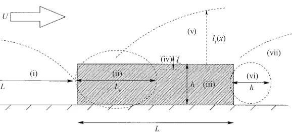
Figure 3. Characteristics of the adjustment to the canopy. (i) Impact region; (ii) adjustment
region (iii) canopy interior; (iv) canopy shear layer; (v) roughness-change region; (vi) exit region; (vii) far wake.
removal of momentum by canopy drag (region (iii) in figure 3). Then from (2.1), (2.3) and (2.5) the mean momentum equation reduces to
0 = d dz
lm2
dU
dz 2
−U2(z) Lc(z)
. (2.8)
The horizontal wind speed within the canopy, U(z), decays with depth from the top of the canopy, where it is Uh, to a very low value within a layer of depth ls, which
can be estimated from (2.8). The turbulent stress gradient is then of the order
d dz
lm2
dU
dz 2
∼ 1 ls
l2m
Uh
ls
2
, (2.9)
and the canopy drag scales asU2/Lc∼Uh2/Lc, so equations (2.8) and (2.9) yield
ls ∼
lm2Lc
1/3
so that ls/ he∼(lm/ he)2/3(Lc/ he)1/3. (2.10)
Hence,ls is controlled partly by the mixing lengthlm, which determines the efficiency
of the turbulence to mix momentum down into the canopy, and partly by the canopy-drag length scaleLc, which determines the efficiency of the canopy to remove
momentum.
Now, increasing the canopy element density increases the canopy drag, and so tends to decrease Lc. In addition, the wake turbulence generated by the additional canopy
elements leads to an enhanced rate of turbulence dissipation (Ayotte, Finnigan & Raupach 1999), which tends to reduce the mixing length lm. From (2.10), these two
tendences both tend to reduce ls and increase the mean shear which has two effects
on the turbulence:
First, vorticity within this shear layer fluctuates in response to vorticity associated with large boundary-layer eddies above the canopy. This shear sheltering (Hunt & Durbin 1999) tends to block the large boundary-layer eddies, which explains why, in measurements above urban areas (e.g. Rotach 1993), the eddy scales for vertical transport, and hence also the mixing length, increase linearly from the blocking shear layer, i.e.
lm=κ(z−d) when z > d. (2.11)
(1971) and proposed by Jackson (1981). The measurements of Rotach (1993) and Raupach, Thom & Edwards (1980) suggest that this mechanism operates even when the canopy consists of obstacles with finite aspect ratios (he ∼be), so that there are
large recirculations in the wakes of the canopy elements. Canopies dense enough that the turbulence structure is changed from the form (2.6) for very sparse canopies, to either of the forms (2.12) or (2.13) we refer to asdense canopies.
Secondly, the shear layer at the top of the canopy is itself dynamically unstable (as observed by Louka, Belcher & Harrison 2000) and produces turbulent eddies characteristic of free shear layers, whose length scales are about equal to the thickness of the shear layer (Raupach et al. 1996; Finnigan 2000). Finnigan & Brunet (1995) show that the shear-layer motions are only weakly coupled to the large-scale boundary-layer eddies above the canopy, in agreement with the idea of shear sheltering. The movement of these inhomogeneous and non-Gaussian eddies down into the canopy mean that these shear layer motions provide much of the energy of the turbulence through the depth of the canopy (Finnigan 2000). Thus, within the canopy, the mixing length,lm, scales on the size of these shear-layer eddies
and is approximately constant, saylm=lc, with height.
If the canopy consists of roughness elements of approximately uniform dimensions or if the canopy consists of roughness elements whose breadths,be, are much smaller
than the thickness of the shear layer, i.e.bels, then the mixing length,lm, is constant
with height and proportional to the thickness of the shear layer, i.e.
lm =lc∝ls whenz < d. (2.12)
Canopies consisting of roughness elements of highly irregular shapes induce large vortical wakes that interact with the downstream elements (e.g. Britter & Hunt 1979). The mean spatially averaged shear layer then ceases to control the dynamics of the turbulence. Instead, the mixing length is controlled by the vortices shed in the obstacle wakes, which are of orderhe:
lc∝he. (2.13)
This value is very much greater than the value in the turbulent boundary layer above the canopy, where lm = κ(z−d). The wind shear is then much smaller within the
canopy, so that the wind profile is more uniform with height.
At the bottom of the canopy, very close to the ground, the eddies are blocked by the ground, so that, as in turbulence near any plane surface,
lm=κz. (2.14)
For a dense deep canopy, wherehels, Inoue (1963) has shown that the solution
to (2.9) is
U =Uhexp ((z−he)/ ls), (2.15)
withls= (2lc2Lc)1/3, which confirms the scaling (2.10) for this particular case.
For a finite-depth canopy, wherehe6ls, the exponential solution is approximately
valid in the upper portion of the canopy. However, near the ground, where κz < lc,
the wind speed is small, i.e.U2/L
cdτ/dz, so that the mean wind profile is close to
a classical logarithmic form. The wind speed near the ground can then be estimated to be
U(0)≈Uhexp (−he/ ls). (2.16)
This leads to the useful distinction between of shallow canopies where ls/ he =
with larger lc ∼ he, the average wind profile is more uniform with height, whence
(2.16) shows how the surface winds are higher. Urban canopies tend to be shallow, whereas vegetation canopies tend to be deep.
Given these arguments, two models are used here to parameterize the mixing length in the analysis of adjustment to a canopy, see figure 2. First, for very sparse canopies we use the standard mixing-length model, which increases linearly from the ground according to (2.6). Secondly, for dense canopies we use the displaced mixing-length
model, which is constant within the canopy and then increases linearly with height
above the shear layer at the top of the canopy, namely
lm=lc when z < zc,
lm=κ(z−d) when z > zc. (2.17)
The region close to the ground in the dense canopies is neglected in the present study.
3. Characteristics of adjustment of the boundary layer to a canopy
Before developing a quantitative model for the adjustment of the boundary layer to a canopy, scaling arguments are developed to show the characteristics of the adjustment and to interpret the quantitative results obtained in §4 below for the linearized model. The adjustment is found to proceed through distinct regions, which are shown schematically in figure 3. The controlling dynamics of these regions and their magnitudes are estimated from the momentum equations.
The drag of the canopy elements acts as an impulse decelerating air parcels, which increases the mean pressure within the canopy. Hence, there is a pressure gradient that decelerates the flow within animpact regionthat extends upwind of the canopy, denoted (i) in figure 3. By continuity, the deceleration of the streamwise flow leads to a vertical motion over and out of the canopy. This mean vertical motion transports fluid upwards, and may be greater than vertical transport of momentum by turbulence in regions (i) and (ii).
From the leading edge of the canopy, within an adjustment region, denoted (ii) in figure 3, the wind within the canopy is decelerated by the canopy drag. The deceleration is largely inviscid and so the canopy drag is largely balanced by streamwise advection. The streamwise lengthscale of the adjustment region can therefore be estimated by balancing the nonlinear drag with the nonlinear streamwise advection, namely
U∂U ∂x ∼
U2 Lc
. (3.1)
The kinetic energy in the mean streamwise velocity, U2/2, is therefore reduced
approximately exponentially on a lengthscale Lc/2 (cf. Finnigan & Brunet 1995).
Thus, the canopy lengthscale, Lc, represents the streamwise distance required for the
canopy to rob an air parcel of its kinetic energy, and hence gives an estimate for the distance for the winds within the canopy to adjust. Deceleration of the streamwise velocity leads, by continuity, to a vertical flux out of the top of the canopy within this adjustment region. Meanwhile, turbulent stresses transport momentum downwards into the canopy.
and (2.16). As described in§2.2, there is a layer of shear of thicknessls between the
canopy flow and the boundary-layer flow above, denoted (iv) in figure 3. The spatially averaged flow above the canopy requires separate consideration with the effect of the canopy being represented by an effective roughness length,z0eff. An internal boundary layer develops in region (v) above the canopy,z > he. Its depth,li(x), is determined,
following Townsend (1965), by balancing streamwise advection and vertical transport by the turbulent stress to yield
liln
li zeff0
≈2κ2(x−x0). (3.2)
Notice how the canopy affects li through the effective roughness length, z eff 0 , and
through the effective origin,x0. At the effective origin for this internal boundary layer, x0, there is a smooth transition from vertical transport driven by the mean velocity
out of the canopy,w(z=he)∼Uh(he/Lc) exp(−x/Lc), to that driven by the vertical
transport by turbulence. Hence, we identifyx =x0 where w(z=he)∼u∗. It follows
that
x0 ∼Lcln
Uh
u∗ he Lc
. (3.3)
Thus, there is a smooth transition a distance of orderx0 downstream of the canopy
edge. If the canopy is exceptionally long, the boundary layer above may fully adjust to the effective roughness of the canopy.
Just above the canopy elements, within the roughness sublayer, there are also time-averaged motions associated with the flow around individual roughness elements. Point measurements (rather than spatially averaged measurements) yield the internal boundary-layer structure only whenli has grown higher than the roughness sublayer,
which typically has depth 2–3he (e.g. Rotach 1993; Louka et al. 2000). Cheng &
Castro (2002b) have shown how this occurs considerably downstream of the leading edge of the canopy. Nevertheless, these complications of the roughness sublayer are avoided when the spatially averaged flow is considered, as it is here.
In the vicinity of the downstream edge of the array is theexit region, denoted (vi) in figure 3. Here, the resistance of the canopy suddenly disappears. There is therefore a force imbalance on the mean flow belowhe and the mean wind accelerates, leading,
by continuity, to a downwards mean vertical velocity. Turbulent stresses transport further momentum downwards to fill the velocity deficit in the wake over a streamwise length scale of orderheUh/u∗.
Yet further downstream is thefar wake region, denoted (vii) in figure 3, where the dynamics is dominated by streamwise advection and downward momentum transport by turbulent stresses. The flow develops in a similar way to the wake behind a single bluff obstacle on a surface. Hence, the wake-velocity deficit,u, is expected to develop asu∝heUh/x, and the height of the wake,hw(x), increases approximately
ashw∝(xhe)1/2 (Counihan, Hunt & Jackson 1974). Sufficiently far downstream, the
boundary layer returns to its far upstream profile.
4. A linear model for adjustment to a canopy
available from the JFM office.) The force distribution is localized around the origin of coordinates and varies over a characteristic horizontal length scaleLand maximum heighthe(see figure 2). The incident wind profile is logarithmic with roughness length z0 and friction velocity u∗. In the following analysis, we calculate changes to the
boundary layer induced by aweak canopy,L/Lc1, so that changes to the boundary
layer are small and therefore can be calculated from the linearized momentum equations. Subsequently, these linear solutions are iterated numerically to obtain changes for denser canopies.
4.1. Governing equations
Each physical quantity, for example the spatially averaged velocity components, Ui,
pressure,P, and stress tensor,τij, is written as the sum of the incident profile, which
would exist in the absence of any canopy and which is denoted by subscript 0, and a perturbation part induced by the canopy, which is denoted by lower case letters. The streamwise velocity component, for example, is then written U =U0+u.
The equations are then linearized for small perturbations by neglecting products of perturbation quantities. On retaining only the dominant Reynolds stress term, namely the shear stress, the equations governing these linearized perturbations become
U0 ∂u ∂x +
dU0
dz w+ ∂p ∂x =
∂τ ∂z −f,
U0 ∂w
∂x + ∂p ∂z = 0, ∂u
∂x + ∂w
∂z = 0. (4.1)
On elimination of the pressure, these equations combine to yield
U0
∂2w
∂z2 + ∂2w
∂x2
−U0w= ∂f ∂z −
∂2τ
∂z2. (4.2)
The boundary conditions are first that the perturbations decay far from the canopy and secondly no-slip at the surface. This is justified even within the canopy because the spatially averaged wind, namelyU0+u, is defined to be the wind averaged within
the fluid volume only, where the no-slip condition is satisfied.
The mixing-length model is also linearized to yield a relationship between the perturbation stress and the perturbation velocity gradient:
τ = 2u∗lm∂u/∂z. (4.3)
As explained in§2.2, the mixing length is parameterized either as the standard mixing length (2.6) or the displaced mixing length (2.17).
The range of validity of the linearized equation (4.2) is established by estimating the magnitude of the linear perturbations compared to the magnitude of the upstream flow. The characteristic velocity scale in the incident flow is Uh, defined at the height
of the canopy, so that
Uh=U0(h) = (u∗/κ) ln(h/z0). (4.4)
following linear estimate for the velocity perturbation
u∼UhL/Lc. (4.5)
Hence, for aweak canopy, withL/Lc1, the perturbation velocities are small,uUh,
and the linearized equation (4.2) is appropriate.
Secondly, as is usual in these perturbed boundary-layer problems (e.g. Townsend 1976, p. 307; Belcher & Hunt 1998), the stress gradient term is smaller than the acceleration term over significant regions of the flow. This can be shown by examining the ratio of these two terms over vertical and horizontal length scales L. In the particular case when the mixing-length model is used:
∂τ/∂z U0∂u/∂x
= (∂/∂z) (2u∗lm∂u/∂z)
U0∂u/∂x ∼
u∗/ lm Uh/L
1. (4.6)
Asymptotic methods can then be used to obtain solutions to (4.2) in the limit that u∗/Uh is small. Now the definition ofUh shows that the analysis requires
u∗ Uh
= 1
(1/κ) ln(h/z0)
1, (4.7)
which is usually satisfied because the upwind roughness length is much smaller than the height of the canopy.
It is convenient to treat the resulting mathematical problem in Fourier space, defined, for example, for the streamwise velocity perturbation, ˜u(k, z), by
u(x, z) = 1 2π
∞
−∞
˜
u(k, z)eikxdk. (4.8)
Application of this Fourier transform to the equation governing the vertical velocity, (4.2), yields
U0
d2w˜
dz2 −k 2w˜
−U0w˜ = d ˜f dz −k
2˜τ− d2τ˜
dz2. (4.9)
With the mixing-length model for the turbulent shear stress, (4.9) becomes a fourth-order ordinary differential equation. There are four boundary conditions: u, w are zero at the surface and u, w decay to zero far above the canopy. Solutions to this equation correspond to the vertical velocity induced by a force that varies sinusoidally in the x-direction about a zero mean. In the linear model, the force variation in the vertical and horizontal directions have to be specified. Solutions for flow through a canopy that varies arbitrarily in the streamwise direction are obtained by numerical inversion of the Fourier transforms.
4.2. The inviscid approximation to the impact and adjustment regions
As shown above, the shear stress is much smaller than the inertial terms over much of the flow. A first approximation to the flow is then calculated by solving (4.9), neglecting the two terms involving the shear stress. A further approximation is to neglect the curvature in the incident wind profile,U0/k2U0, which is small away from
the surface in a logarithmic incident profile. Solutions based on these approximations are described in§4.2.1 and§4.2.2.
generalization of the inviscid theory can provide insights into the effects of the finite volumes of the canopy elements.
4.2.1. General solution in the inviscid approximation
Equation (4.9) is approximated as described above, when it reduces to (the Fourier transform of) Poisson’s equation. The resulting equation can be solved using Green’s function methods to give
˜
w=Ce−kz+ Dekz+
z
z0
˜
f(k, z)cosh (z−z
)
U0(z)
dz, (4.10)
where C and D are coefficients determined by boundary conditions (the notation is chosen to be consistent with Jerram 1995, chapter 3). The solutions for the streamwise velocity and pressure perturbations are then found from continuity and the streamwise momentum equation, respectively, to yield
˜
u=−iCe−kz+ iDekz− f˜ ikU0(z)
+ z
z0
˜
f(k, z)sinh (z−z
)
U0(z)
dz (4.11)
˜
p= iU0(z)
Ce−kz−Dekz−
z
z0
˜
f(k, z)sinh (z−z
)
U0(z)
dz
. (4.12)
The coefficient D is determined by the condition that the perturbations decay far from the canopy, which implies that
D+ 1 2
∞
z0
˜
f(k, z) e−
kz U0(z)
dz= 0. (4.13)
The second coefficient,C, is determined with the boundary condition that the vertical velocity is zero at the surface,z=z0, which yields
C+D= 0. (4.14)
Higher-order corrections to this leading-order solution that account for small, but finite, curvature in the upwind velocity profile have been derived (Jerram 1995,§3.5.7).
4.2.2. Inviscid solution for a rectangular canopy
For a constant drag in a rectangular region, lying between x= −L/2 and L/2, namely
f = U
2 h Lc
{H(x+L/2)− H(x−L/2)} {1− H(z−he)}, (4.15)
where H is the Heaviside step function, the solutions can be evaluated explicitly in physical space to yield
u(x, z) = UhL/Lc 4π
h1
ˆ
x−12,zˆ−hˆe
−h1
ˆ
x+ 12,zˆ−hˆe
−h1
ˆ
x− 12,zˆ+ ˆhe
+h1
ˆ x+1
2,zˆ+ ˆhe
−4π(1− H(z−he))
, (4.16)
w(x, z) =−UhL/Lc 4π
h2
ˆ
x−12,zˆ−hˆe
−h2
ˆ
x+12,zˆ−hˆe
−h2
ˆ
x− 12,zˆ+ ˆhe
+h2
ˆ x+1
2,zˆ+ ˆhe
–2 –1 0 1 2 0
1 2
z L
2x/L
Figure 4.Inviscid perturbations, u/Uh, to a uniform incident flow, Uh, at a succession of
downstream locations through a canopy with constant drag force,f = 0.45U2
h/Landh/L= 0.5
(so thatL/Lc ≈0.5). Note the non-zero perturbation at the surface and the discontinuity inu
at the top of the canopy. At the end of the canopy and in the wakeu/Uh=−0.83.
Here, ˆx=x/L, ˆz=z/L, ˆhe=he/L and
h1(ξ, ζ) =ζln
ξ2+ζ2−2ξtan−1(ξ /ζ), (4.18)
h2(ξ, ζ) =−ξln
ξ2+ζ2−2ζtan−1(ξ /ζ), (4.19)
where the inverse tangents are defined to lie within −π/2 and π/2, so that care is needed in evaluating the solutions across the branch cuts around the boundary of the canopy.
We have argued that over significant regions of the flow, the solution is dominated by inviscid irrotational processes. Hence, figure 4 shows profiles of the streamwise velocity as a uniform flow,Uh, impinges upon a rectangular canopy with a constant
resistive force,f = 0.45U2
h/L, calculated using the inviscid solution (4.16). The solution
shows clearly how the wind speed decelerates in the impact region, and within the canopy, with an increasing velocity deficit through the canopy. Above the canopy, the wind speed is decelerated and then beyond halfway, it is accelerated: the canopy acts as a source above the canopy. In the inviscid approximation, the drag-induced velocity deficit remains constant in the wake downwind of the canopy and does not decay.
The solution (4.16) and the profiles in figure 4 show that upwind of the canopy, within the impact region, the flow decelerates over a length of order L. Just at the upwind edge of the canopy at the surface the inviscid solution (4.16) gives
u(−L/2, z0) =Uh
− 1
2π
he Lc
ln
h2 e+L2
h2 e
+ L
4πLc
4 tan−1
L 2he
−2π
≈ −Uh
2π
he Lc
ln
1 +L
2
h2 e
, (4.20)
when the canopy is long,Lhe, so that 4 tan−1(L/2he)→2π.
This result is from the linear solution, which requires L/Lc1. The deceleration
is comparable to or greater than Lc, only in the adjustment region is there a mass
flux out of the canopy. Downwind, there is a slowly varying weak flow within the canopy (ifhe>ls). Hence, an estimate for the deceleration upwind of the canopy for
more typical canopies that haveL>Lc that accounts for this nonlinear process (but
ignores others) is obtained by replacingLwith Lc in (4.20) to yield
u(−L/2, z0) =− Uh
2π
he Lc
ln
1 +L
2 c h2 e
. (4.21)
Later this expression will be compared to measurements.
4.2.3. Effects of canopy elements of finite volume in the impact region
The analysis developed above shows how the aerodynamic resistance of the roughness elements within the canopy decelerates the flow over a distance of order L upwind of the canopy and leads to a velocity perturbation (4.21) just upwind of the canopy. Now, when the canopy elements have a finite volume, the streamlines are also displaced over and around the canopy elements. This displacement also leads to a deceleration of the (spatially averaged) mean flow, U.
The magnitude of this deceleration can be estimated by calculating the inviscid irrotational perturbations to a uniform upwind flow, of magnitude Uh, caused by a
set of obstacles mounted on a surface. The resulting potential flow induced by the bodies is then averaged over a horizontal area (ge+be)×(ge+be) to estimate the
deceleration of the mean flow induced by an canopy of elements of finite volume. If the canopy elements are either cuboidal, so thatbe∼we∼he, or tall thin cylinders
mounted vertically, so thatbeheand the flow is predominantly around the obstacles,
then the perturbation velocity near the surface a distance (ge+be) upwind of the
canopy is of order
u Uh
∼ − b2e
(ge+be)2
, (4.22)
and the deceleration decays algebraically upwind of the canopy on the length scale ge+be.
We shall see evidence in the comparisons with measurements described in §5 of these decelerations associated with the finite volumes of the canopy elements.
4.3. Effects of the turbulent stress gradients
As the profiles in figure 4 show, the inviscid solution is incorrect both at the surface, because it does not satisfy the no-slip condition, and at the top of the canopy, where discontinuity in the force distribution yields large vertical gradients in the streamwise velocity perturbations. Within thin layers, referred to here as inner layers, centred at these two levels, the turbulent shear stress gradient become comparable to the inertial terms, and a new analysis is required.
Following analyses of flow over hills (Jackson & Hunt 1975; Belcher & Hunt 1998; Hunt, Leibovich & Richards 1988) and flow over roughness changes (Belcher et al.
1990), the stress gradient and advection terms, namely the first and sixth terms in (4.9), are comparable in the inner layers, which on using the linearized version of the mixing-length model (4.3) yields
− d2 dz2
2κu∗z
ik d2w˜
dz2
∼U0(z)
d2w˜
If the inner layer is centred at heighthi, (4.23) yields an estimate for the thickness,li,
of the inner layer, namely
k2li2∼khi u∗ U0(hi)
. (4.24)
The inner layer at the ground within the canopy, where the wind velocity decreases to zero to satisfy the no-slip condition, then hashi =li, so that kli ∼u∗/U0(li), which is
small. The inner layer at the top of the canopy hashi =he, so thatk2li2∼kheu∗/Uh,
which is also small. Hence, the inner layers are thin. This means first that, within the inner layers, streamwise gradients,∂/∂x, can be neglected compared with vertical gradients, ∂/∂z. Secondly, the shear in the incident wind profile is small in the thin inner layers and so the value of the incident wind profile can be approximated by its value at the layer height, i.e. U0(z) ≈ U0(hi). Thirdly, the curvature term in (4.9) is
smaller within the inner layer than the advection term because their ratio is small:
U0w˜ U0d2w/˜ dz2 ∼
u∗ U0(hi)
1. (4.25)
Hence, to leading order, the flow in the inner layers is governed by
− d dz
d dz
2κu∗lm
ik d2w˜
dz2
−U0(hi)
d ˜w dz
= d ˜f
dz. (4.26)
This equation can be integrated once with respect to z. The integration constant is ikp˜(hi), the perturbation pressure, which is approximately constant with height over
the thin inner layer. On using continuity, d ˜w/dz=−iku˜, the leading-order equation governing dynamics of inner layers, becomes
d dz
2κu∗lm
d˜u dz
−ikU0(hi)˜u= ˜f + ikp˜(hi). (4.27)
Hence, any imbalance between streamwise advection, canopy drag and the pressure perturbation driven by the inertial forces is balanced by vertical transport of momentum by the stress gradient. The solution to (4.27) depends on the model used for the mixing length. Explicit solutions for the standard mixing length and the displaced mixing length are developed next.
4.3.1. Solution with the standard mixing-length model
As described above, for a uniform canopy of depthhethere are inner layers around
the top of the canopy, z=he, and at the surface z= 0. Focus initially on the inner
layer at the surface.
The most general solution to (4.27) is found using Green’s function methods, and with the standard mixing-length model,lm=κz, Jerram (1995,§ §3.5, 3.6) shows that
˜
u=AJ0(Z) +BK0(−iZ)−
˜ p U0(hi)
− 1
ikU0(hi)
Z
Z0
Zf˜(k, z){J0(Z)K0(−iZ)−J0(Z)K0(−iZ)}dZ, (4.28)
whereJ0(Z) andK0(−iZ) are Bessel functions (Abramowitz & Stegun 1972, chapter 9).
The first,J0(Z), increases exponentially for largeZ and the second, K0(−iZ), decays
variable defined by
Z= exp (3iπ/4)
U0(hi) κu∗ kz
1/2
. (4.29)
Note how ˜f in (4.28) remains a function of the unscaled heightz.
The coefficients Aand Bin (4.28) are determined by the boundary conditions. Far above the inner layer, the solution must remain finite, so that the coefficient ofJ0(Z)
must be zero at largeZ, which yields
A− 1
ikU0(hi)
∞
Z0
Zf(k, z)K0(−iZ) dZ= 0. (4.30)
Towards the surface, J0(Z) tends to zero, whereas K0(−iZ) diverges logarithmically.
The logarithmic divergence is avoided, and the no-slip condition is satisfied for the inner layer at the surface, ifB satisfies
AJ0(Z0) +BK0(−iZ0)−
˜ p(hi) U0(hi)
= 0, (4.31)
whereZ0 is the value of Zat z=z0.
The final condition required to determine the final coefficient in (4.10) and (4.28), namely ˜p(hi), is obtained by calculating the pressure in the inner layer, which is
determined from the solution for the pressure in the inviscid layer (4.12) taken in the limit of smallz. This procedure yields
˜
p(hi) = iU0(hi)(C−D), (4.32)
whereC is given by (4.14) andDis given by (4.13).
The inner layer around the top of the canopy has formally the same solution, namely (4.28), but with di = he. Both inner layers are then neatly accounted for if U0(hi) is replaced byU0(z) throughout the solutions to the inner layer obtained above.
Hence, all the coefficients are determined: (4.13) determines D, (4.14) determines C, (4.30) determinesA, (4.31) determinesB, and (4.32) determines ˜p(hi). The solution
with the standard mixing-length model is then complete. Jerram (1995,§3.5.8) shows that the small downstream thickening of the inner layer leads to a small vertical velocity, so that when higher-order linear effects are calculated, C+D in (4.14) has a very small contribution, of orderu2
∗/Uh2.
4.3.2. Solution with the displaced mixing-length model
With the displaced mixing-length model, in the flow through the bulk of the canopy,z < zc, the mixing length is constant and so, in the linearized framework, the
perturbation flow is governed by a constant viscosity, namely νt = 2κu∗lm. Solutions
for the perturbations to the flow within the canopy can then be calculated from (4.2) with no further approximation.
Hence, following Jerram (1995, §3.8.5), the solution to (4.2) in z < zc is calculated
using Green’s function methods, and is found to be
˜
w=E[sinh{α(z−z0)} −(α/β) sinh{β(z−z0)}]
+F[cosh{α(z−z0)} −cosh{β(z−z0)}]
− ik 2κu∗lm
z
z0 ∂f ∂z(k, z
)
sinh{α(z−z)} α(α2−β2) −
sinh{β(z−z)} β(α2−β2)
Hereα2=k2+ ikU
h/νt andβ=|k|, andE andF are coefficients that are determined
by boundary conditions. The streamwise velocity perturbation is obtained from continuity and the pressure perturbation from the streamwise momentum equation, thus
˜ u=−1
ik ∂w˜
∂z, (4.34)
˜
p=−2κu∗lm k2
∂3 ∂z3 −k
2 ∂ ∂z
˜ w+ Uh
ik ∂w˜
∂z + ˜ f
ik, (4.35)
˜
τ =−2κu∗lm ik
∂2 ∂z2 −k
2
˜
w. (4.36)
Above zc, the mixing length increases with height, lm = κ(z−d), where d is the
displacement height. Hence, the solution here has inner-layer dynamics, and so the approximate solution is formally the same as (4.28), but with the height z replaced by the displaced heightz−d. Hence, the solution is (4.28) with
Z= exp (3iπ/4)
U0(hi)
κu∗ k(z−d) 1/2
. (4.37)
The two coefficients,A and B, in this solution are determined by matching with the inviscid layer that applies above the inner layer at the top of the canopy, and proceeds exactly as in §4.3.1. The inviscid component of the solution is also written in terms ofz−d, namely
˜
w=Ce−k(z−d)+Dek(z−d)+
z−d
z0
˜
f(k, z)cosh (z−z) U0(z)
dz. (4.38)
The inner-layer solution must also match with the solution in the canopy mixing layer, where the velocity perturbations are ˜uc and ˜wc. Hence, the solutions above
the canopy mixing layer are the same as with the standard mixing-length model but with an effective origin at the displacement heightz=d, and with additional velocity perturbations ˜uc and ˜wc. The remaining constants E and F, which can be related to
˜
uc and ˜wc, are found by ensuring that ˜pand ˜τ are continuous at the top of the layer
of constant mixing length. In the solutions calculated here, these coefficients were calculated numerically: the procedure is straightforward but lengthy, for details, see Jerram (1995,§3.8.7).
4.4. Numerical implementation
The solutions derived above are for the Fourier transforms of the perturbations to the flow induced by a weak force distribution, with Fourier transform ˜f(k, z). The procedure for obtaining solutions for a realistic force distribution that varies in the streamwise direction,f(x, z) is as follows. The Fourier transform is taken numerically of the force distribution,f(x, z), to yield ˜f(k, z). The solutions obtained above, which depend upon ˜f(k, z), are then evaluated numerically for each k. These solutions for the Fourier transforms of the perturbation flow, e.g. ˜u(k, z), are then inverted numerically using a fast Fourier transform to obtain the perturbations in physical space according to (4.8).
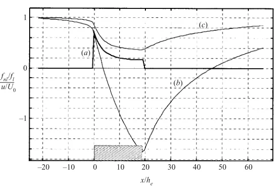
–20 –10 0 10 20 30 40 50 60 –1
0 1
x/he
(a)
(c)
(b)
fnl/fl u/U0
Figure 5. The effect of iterating the force. (a) The ratio of the force after iteration to
before iteration, integrated over the height of the canopy. (b,c) Streamwise velocity at half the canopy height, before and after iteration, normalised on undisturbed wind speed at half the canopy height. The horizontal axis is streamwise distance from leading edge normalised on the canopy height. The position of the canopy is shown as hatched.
force distribution is such that−∞∞ f(x, z) dx= 0, which is not typical.) The singularity is treated by integrating the small-wavenumber range separately by changing the integration variable to lnk. See Jerram (1995,§4.3) for details.
Finally, as explained in §2.1, the force distribution is written for practical applications as f = U2/Lc. In a strictly linear analysis, the forcing then becomes f = U02/Lc with U0(z) the upstream undisturbed velocity profile. With this strictly
linear model, the flow can never adjust to a balance between the stress gradient and the canopy drag, because the canopy drag does not adjust. Hence, such a strictly linear model can only describe the adjustment region described in§3.
The strictly linear model can be improved upon significantly by accounting for the nonlinear drag, yielding a quasi-linear model. The procedure is to iterate numerically the linearized solutions obtained analytically as follows. On the first iteration, f is specified using the undisturbed velocity profile U0(z). The streamwise velocity
perturbations are then calculated. A new force distribution is then constructed using the computed streamwise velocity U0 +u. This force distribution is then used in
the analytical solutions to compute the next iteration for the streamwise velocity perturbation. The process is repeated until the solution changes by less than a specified tolerance. In the examples considered below, the solutions converged in three or four iterations.
5. Comparison of model results with previous studies
The objective of the present study has been to elucidate scalings for adjustment to a canopy and also to develop a quantitative model. Therefore, any parameters of the model are estimated on the basis of physical arguments, the flow that result from the estimated parameter set is then calculated, and the results compared with simulations or experiment.
Each of the comparisons below shows a different aspect of the fluid dynamics:§5.1 shows how the quasilinear model compares with a numerical model with all nonlinear terms;§5.2 shows adjustment to a fine-scale (forest) canopy;§5.3 shows recovery and then impact in a fine-scale canopy; and§5.4 shows adjustment to a canopy of large roughness elements, when we suggest the finite-volume process becomes important.
5.1. Comparison with the numerical model of Svensson & H¨aggkvist
Svensson & H¨aggkvist (1990) performed a numerical simulation of two-dimensional mean flow through a distributed resistance in a rectangular region with he = 2.5 m
andL= 250 m. The distributed resistance was calculated fromf = ¯cda|U|U/2, with
a drag coefficient ¯cd = 0.3, and a ‘plant area density’, a = 2.1 m−1, which yields Lc= (¯cda/2)−1= 3.2 m, so thathe/Lc= 0.8. This is a shallow canopy.
The turbulent stress was modelled by Svensson & H¨aggkvist using a modified form of thek−εclosure model. Small-scale wake turbulence generated by the canopy increases small-scale dissipation (Kaimal & Finnigan 1995, chapter 3), which Svensson & H¨aggkvist represent by introducing new source terms based on ¯cd, a and U into
the equations for turbulent kinetic energy and turbulent dissipation. Svensson & H¨aggkvist adjusted the coefficients multiplying these new source terms to give good agreement with canopy velocity profiles measured in the experiment of Raupachet al.
(1986) far downstream of the adjustment region.
The incident velocity profile used by Svensson & H¨aggkvist was
U(z) = 10
z 110 m
1/7
m s−1. (5.1)
For comparison with the present model, a logarithmic profile was fitted to (5.1) by matching velocities at z=he and z=he/2. This gives z0 = 1.604 mm and u∗ =
0.3248 m s−1. The fitted logarithmic profile then differs from (5.1) by less than 3%
over the height range 0.4 m< z <11 m, which includes the part of the canopy where the distributed force and velocity perturbations are most significant.
The present model, with the simple mixing length, was used to compute the flow through a rectangular canopy. Results in the exit region of the canopy calculated from the present model are compared with Svensson & H¨aggkvist’s results in figure 6. The points are simulation data measured from Svensson & H¨aggkvist’s figure 4a. The curves are from the present model. The agreement is satisfactory, giving confidence that the quasi-linear model developed here is useful in representing the nonlinear adjustment computed by Svensson & H¨aggkvist’s fully-nonlinear model.
5.2. Flow through a model plant canopy
Meroney (1968) measured the turbulent flow in and above a model forest consisting of trees made from ‘plastic simulated-evergreen boughs’. His forest canopy was 0.18 m high and 11 m long with tree density one per 36 cm2. Meroney gives the tree drag
coefficient as ¯cd = 0.72 and his description of the model tree shape gives a frontal
area of 71.5 cm2. Hence, the projected frontal area of the tree crown isa
f = 11.0 m−1.
x (m)
20 40 60 80 100 120 140 160 180
0 2 4 6 8 10 12 14
z (m) U0 + u
Figure 6. Profiles of streamwise velocity in the exit region of a canopy, whose position is
shown as hatched. Points: numerical simulation of Svensson & H¨aggkvist (1990). Curves: current theory with the simple mixing-length model.
and orientation within the crown. The occupied volume fractionβ is half the volume porosity of the tree crown. In the absence of more precise information, we estimate a/(1−β) =af. With this data, and assuming that the drag is uniformly distributed
with height, the canopy-drag length scale is estimated from (2.4) to be Lc = 0.13 m.
Hence,he/Lc= 1.4 and this is a deep canopy, typical of forests. Jerram (1995,§4.7)
also shows calculations with a higher drag in the tree crown than in the trunk space. The results are almost indistinguishable from the results with the uniform drag and are not further discussed here.
Meroney did not specify an incident velocity profile. It is estimated here by fitting a logarithmic profile to his measured profile at x = −1 m. This gives z0 = 1.77 mm
and u∗ = 0.391 m s−1. The present model was also used to compute the flow using
the displaced mixing-length model. The parameters for the displaced mixing-length model are estimated to be lc/ he = 0.2, d/ he = 0.7 and zc/ h= 0.75. The low value
oflc/ he reflects the small horizontal length scale of the model forest elements (which
were less than about 5 cm) in comparison with canopy height. The value ofd/ heis an
estimate following Thom (1971) and Jackson (1981) of the level of mean momentum absorption, and is typical of the ratios observed. These values ofzc andd imply that
the effective roughness length of the canopy is zeff0 = 0.05he≈1 cm.
The comparison between present theory and experiment is shown in figure 7 (simple mixing-length model) and figure 8 (displaced mixing-length model). In general, the agreement is good, and more so for the downstream half of the canopy than for the upstream half. Note also that the deceleration of the flow ahead of the canopy obtained from (4.21) isu/U0 =−0.24, which is about a quarter of the maximum velocity deficit
in the canopy, in agreement with the computations and the measurements.
x = 0
li
–1 0 1 2 3 4 5 6 7 8 9 10 11
x (m) x = L
0 0.5 1.0
z (m)
z = he
Figure 7.Profiles of perturbations to the streamwise velocity through Meroney’s (1968) wind
tunnel model of a forest canopy. Points: values measured by Meroney (1968). Solid lines: current theory using the simple mixing-length model. Dotted line: boundary of the canopy; dot-dash line: sketch of the development of the internal boundary layer that develops over the canopy interior.
–1 0 1 2 3 4 5 6 7 8 9 10 11
x (m) 0
0.5 1.0
z (m)
Figure 8.Comparison of Meroney’s (1968) wind tunnel model of a forest canopy with
the present model using the displaced mixing-length model with lc/ he = 0.2, d/ he = 0.7
and zc/ he = 0.75. Perturbation streamwise velocity is plotted against height at a series of
downstream locations. Points: experimental data. Solid lines: current theory.
5.3. The effect of a clearing in mid-forest
Next the model is applied to a mean wind acceleration in a clearing in mid-forest investigated by Stacey et al. (1994) using model trees in a wind-tunnel experiment. Stacey et al. modelled a spruce forest with average height he = 15 m, with far
–1 0 1 2 3 4 5 6 7 8 9 0
1 2 3
Figure 9. Velocity vectors in a clearing in mid-forest. Coordinates are non-dimensionalized
on the forest canopy heighth= 15 m. Grey scale within the canopy indicates the strength of the local force on the canopy: the largest force acts at the leading edge of the canopy following the clearing.
(1975), namely,
D= 0.4352U2m0.667exp(−0.0009779U2), (5.2) wheremis the tree’s live branch mass in kg andU is the nominal incident wind speed in m s−1. In the conditions being modelled, the live branch mass was m = 49.5 kg
and the nominal wind speed 30 m s−1, hence the drag force on an isolated full-scale
tree was 2193 N. The lateral and streamwise tree spacings were 1.73 m, so the canopy volume per tree was 44.9 m3. Therefore, the canopy adjustment length scale may be
estimated as
1 Lc
= 1 2193 N
2ρ×302m2s−2×44.9 m3
≈0.11 m−1, (5.3)
so thatLc= 9 m and this is again a deep canopy with he/Lc= 1.7.
The flow field shown in figure 9 is calculated using two regions of distributed force. Both are 15 m high and haveLc= 9 m. One extends from x=−500 m tox = 0 and
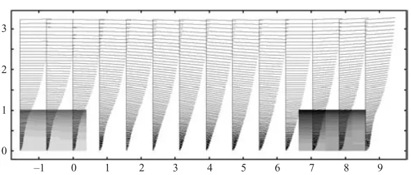
is intended to set up an equilibrium canopy flow. The other extends fromx= 100.5 m tox= 300 m. The clearing lies between the two regions. The experimentally measured flow field is shown in Staceyet al.’s (1994) figure 13. Detailed numerical comparison is not attempted here; there is qualitative agreement between the experimental data presented in Stacey et al. and the present model. The most notable feature is the vertical velocity variation within the clearing. The wind turns downwards to fill out the clearing immediately after its upstream edge and only turns upwards again after the trailing edge when the blocking effect of the downstream resistance has become dominant.
The shaded contours over the canopy regions in figure 9 represent the strength of the local distributed force. The darker contours at the downstream edge of the clearing indicate that the force acting is stronger here than in the equilibrium flow at the left-hand edge of the figure. Hence, a clearing in a forest increases the risk of local wind damage, as observed by Stacey et al.
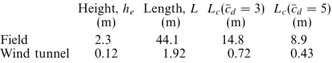
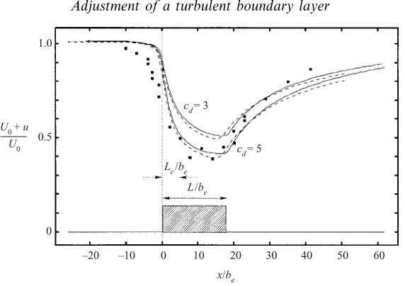
5.4. Deceleration of the mean wind through a building canopy
Davidson et al. (1995a,b) conducted two experiments on a staggered array of obstacles, arranged as shown in figure 10, more typical of an urban canopy with he/Lc < 1. One was a full-scale field experiment with obstacle dimensions (refer to
figure 10) we×be×he= 2.2 m×2.45 m×2.3 m, withL= 44.1 m, the other a