Genetic Analysis of Diallel Tests of Loblolly Pine (Pinus taeda L.)

(1)

BIN XIANG Genetic Analysis of Diallel Tests of Loblolly Pine (Pinus taeda L.)

(Under the direction of Dr. Bailian Li)

A new approach was developed for analyzing diallel tests with SAS PROC MIXED and PROC IML. The new method can estimate variance components, obtain BLUE (best linear unbiased estimators) of fixed effects and BLUP (best linear unbiased predictors) of random genetic effects simultaneously. A new formula based on BLUP was further developed to predict individual tree breeding values. This new analytical method was validated using computer simulation and was compared with other existing programs.

To analyze disconnected diallel mating designs with more than one diallel, simulated data generated with known parameters were analyzed using BLUP to compare three alternative models, which include diallel as fixed effect (Model 1), random effect (Model 2) or no diallel effect (Model 3). Both Model 1 and Model 3 produced unbiased GCA (general combining ability) variance estimates, while Model 2 resulted in downward biased GCA variance estimate. The accuracy of BLUP prediction for three models was very close, with Model 3 slightly better than the other two.

Statistical approaches were also evaluated for combining multiple disconnected diallel test series in a given region. The best GCA sample variance prediction in the class of linear combination of local variance estimates was derived. Simulation study showed that a checklot adjustment was very critical to improve the prediction of genetic values obtained using BLUP analysis. Additional adjustment with improved GCA sample variance prediction could improve the correlation slightly beyond checklot adjustment.

(2)

corresponding heritabilities for height; 3) DBH and volume had higher genetic correlation with 8-year volume than height.

Genetic gain prediction in year-8 volume for selection on height and volume indicated that: 1) selection on volume yielded more gain than selection on height; 2) Coastal population had the greatest correlated response, followed by Piedmont and Northern population; 3) family plus within family selection based on total genetic component can capture the most genetic gain; 4) for all selection methods, additional gain (10-40%) can be achieved by capturing non-additive genetic component.

(3)

(4)

BIOGRAPHY

Bin Xiang was born on December 29, 1970 in Yuyao, Zhejiang Province, China. At the age of seven, he began to receive education at a neighborhood primary school.

The author completed his undergraduate studies at Nanjing University with a Bachelor of Science in Ecology in 1992. At the same year, his graduate studies started at the Institute of Botany, Chinese Academy of Sciences. After three years’ study and research in plant physiological ecology, he graduated with a Master of Science in Botany in 1995.

(5)

ACKNOWLEGEMENTS

The pursuing of PhD degree would not be possible without the guidance, support, coaching and mentoring of my advisor Dr. Bailian Li. He not only guided me through this process but also taught many valuable lessons of the life.

I would like to extend my appreciation to committee members, Dr. Eugene Eisen, Dr. Gary Hodge and Dr. Roger Berger for their time and effort in pursuit of this work. They were always there to offer helping hand throughout the process. I am also grateful to Department of Forestry and the Tree improvement Program at North Carolina State University for funding and supporting this work.

I extend special thanks to my parents Shougen Xiang and Xinhui Wang for their unselfish love and constant emotional support through these years of studies.

(6)

LIST OF TABLES

Table 1-1. Means, standard deviation and percentage bias of estimated variance components for 1000 simulated data sets... 12 Table 1-2. Mean distances of variance component estimated from true variance and from sample variance of simulated effect values for 1000 simulated data sets ... 12 Table 1-3. Mean correlation and standard deviation of true and predicted GCA, SCA and GV (BLUP) for 1000 simulated data sets ... 13 Table 1-4. Comparison of variance components and individual heritability estimated by SAS PROC MIXED, GAREML and DIALL, with different degree of balance. .... 15 Table 1-5. Comparison of GCA estimated by SAS PROC MIXED, GAREML and

DIALL, with different degree of imbalance. ... 16 Table 1-6. Comparison of SCA estimated by SAS PROC MIXED, GAREML and DIALL for the balanced data set. ... 17 Table 1-7. Comparison of SCA estimated by SAS PROC MIXED, GAREML and

DIALL, for the unbalanced data set with 5 missing crosses and 60% survival 18 Table 2.1.1. Parameter structure for generating simulated data sets ... 30 Table 2.1.2. Imbalance levels considered in simulation study ... 31 Table 2.1.3. Summary statistics of σd2 estimate in model 2 from analysis of simulated

data sets (1000 for each parameter structure and imbalance level), including mean, standard deviation (S.D.), Coefficient of Variation (CV), minimum (MIN), maximum (MAX) and 75 percentile ... 34 Table 2.1.4. Percentage bias of σg2 estimate in 3 models from analysis of simulated data sets (1000 for each parameter structure and imbalance level) ... 35 Table 2.1.5. Coefficient of variation (C.V.) of σg2_{estimate and correlation between S}

g2

and σg2_{estimate in 3 models from analysis of simulated data sets (1000 for each}

parameter structure and imbalance level) ... 37 Table 2.1.6. Mean distance of σg2_{estimate in 3 models from analysis of simulated data}

sets (1000 for each parameter structure and imbalance level) ... 38 Table 2.1.7. Mean square error of σg2_{estimate in 3 models from analysis of simulated}

data sets (1000 for each parameter structure and imbalance level) ... 39 Table 2.1.8. Mean distance (MD) and mean square error (MSE) of GCA prediction in 3 models from analysis of simulated data sets (1000 sets for each parameter structure and imbalance level) ... 42 Table 2.1.9. Mean distance (MD) and mean square error (MSE) of GV prediction in 3

(11)

Table 2.1.10. Overall correlation and mean sample correlation between true parental GCA and prediction in 3 models from analysis of simulated data sets (1000 sets for each parameter structure and imbalance level) ... 45 Table 2.1.11. Overall correlation and mean sample correlation between true full-sib

(12)

LIST OF FIGURES

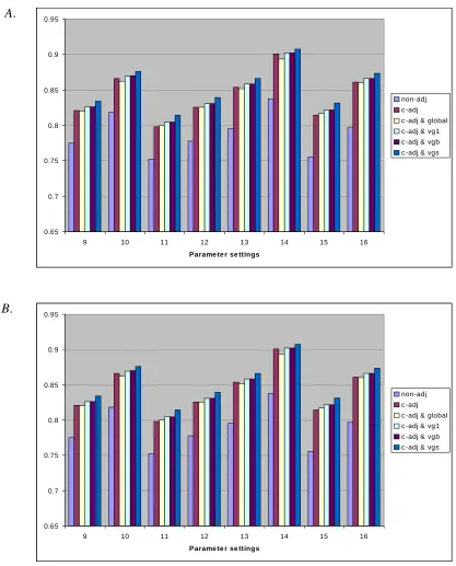
Fig 2.2.1 Different GCA predictions of parent A and B in two test series ... 56 Figure 2.2.2 Two sets of parental GCAs from two test series ... 57 Figure 2.2.3 Mean distance (MSE) of parental GCAs from BLUP analysis of simulated data sets (1000 for each parameter structure) across 4 (A) test series and 8 (B) test series ... 63 Figure 2.2.4 Mean square error (MSE) of parental GCAs from BLUP analysis of

simulated data sets (1000 for each parameter structure) across 4 test series (a) and 8 test series (B) ... 64 Figure 2.2.5 Mean distance (MSE) of full-sib genetic values (GV) from BLUP analysis of simulated data sets (1000 for each parameter structure) across 4 (A) test series and 8 (B) test series ... 66 Figure 2.2.6 Mean square error (MSE) of full-sib genetic values (GV) from BLUP

analysis of simulated data sets (1000 for each parameter structure) across 4 (A) test series and 8 (B) test series ... 67 Figure 3-1. Time trend of additive (σ2

A ) and dominance (σ2D ) variance component

estimates for trait height (HT), diameter at breast height (DBH) and volume (VOL) during early growth period in 3 test regions (Northern, Coastal and Piedmont) ... 84 Figure 3-4. Time trend of narrow sense (h2) and broad sense (H2) individual heritabilities

for trait height (HT), diameter at breast height (DBH) and volume (VOL) during early growth period in 3 test regions (Northern, Coastal and Piedmont) ... 86 Figure 3-5. Time trend of family mean heritabilities for trait height (HT), diameter at

breast height (DBH) and volume (VOL) during early growth period in 3 test regions (Northern, Coastal and Piedmont) ... 87 Figure 3-10 Comparison of age-age correlation of growth traits for 3 test regions: ... 90 Figure 3-11. Comparison of correlation with age 8 volume of growth traits for 3 test

regions ... 92 Figure 4-1. Correlated response of 8-yr volume from various selection methods on height (A) and volume (B) at age 6 in three test regions ... 109 Figure 4-2. Comparison of three test regions in family selection efficiencies of early

height on 8-yr volume base on gain per year criterion (SE1) for three regions ... 112 Figure 4-3. Comparison of different selection methods in selection efficiencies of early

(13)

Figure 4-4. Comparison of three test regions in family selection efficiency of early volume on 8-yr volume base on gain per year criterion (SE1) for three regions ... 116 Figure 4-5. Comparison of different selection methods in selection efficiency of early

volume on 8-yr volume for Coastal population, based on gain per year (SE1) ... 117 Figure 4-6. Comparison of selection efficiency criteria, gain per year (A) vs present value

(B) of early height or volume on 8-yr volume for Northern population 118

Figure 4-7. Selection efficiency of early height on 8-yr volume for Northern population, selection efficiencies of gain per year ... 138 Figure 4-8. Selection efficiency of early height on 8-yr volume for Coastal population,

selection efficiencies of gain per year ... 138 Figure 4-8. Selection efficiency of early height on 8-yr volume for Coastal population,

selection efficiencies of gain per year ... 139 Figure 4-9. Selection efficiency of early height on 8-yr volume for Piedmont population, selection efficiencies of gain per year ... 140 Figure 4-9. Selection efficiency of early height on 8-yr volume for Piedmont population, selection efficiencies of gain per year ... 140 Figure 4-10. Selection efficiency of early volume on 8-yr volume for Northern

population, selection efficiencies of gain per year ... 140 Figure 4-10. Selection efficiency of early volume on 8-yr volume for Northern

population, selection efficiencies of gain per year ... 141 Figure 4-11. Selection efficiency of early volume on 8-yr volume for Coastal population, selection efficiencies of gain per year ... 141 Figure 4-11. Selection efficiency of early volume on 8-yr volume for Coastal population, selection efficiencies of gain per year ... 142 Figure 4-12. Selection efficiency of early volume on 8-yr volume for Piedmont

population, selection efficiencies of gain per year ... 142 Figure 4-12. Selection efficiency of early volume on 8-yr volume for Piedmont

(14)

General Introduction

Loblolly pine is the most important commercial tree crop in the southern United States. It produces over half of the total southern pine wood volume, and it accounts for about 80 percent of all southern pine seedling production in the United States (Lantz et al. 1987). It will become an increasingly important source for softwood fiber for pulp and timber in the future (Mckeand et al. 1997, Li et al 1999).

The North Carolina State University - Industry Cooperative Tree Improvement Program (NCSU-ICTIP) has completed 45 years of loblolly pine tree improvement in the southeastern United States. Through the first two cycles of breeding, testing and selection substantial genetic gains have been achieved. The cooperative’s tree improvement program for loblolly pine is now moving into its third generation (Li et al. 1996,

Mckeand et al. 1997, Li et al 1999). To further implement the third generation and future breeding plans, it is necessary to thoroughly analyze and evaluate current data accumulated from the first and second-generation progeny tests of NCSU-ICTIP.

The analysis of data from the first generation tests indicated time trends in genetic parameters for tree height and suggested that, if a single measurement is used, measurement at age 6 and selection one year later would maximize the gains per year as well as increase the financial returns from seed orchards (McKeand 1988, Balocchi et al.

1993).

(15)

heritability, and provide the progeny population for the next generation of breeding. The expected genetic gain can also be predicted.

With better estimates of parameters, time trends of selection efficiency can be calculated for different selection methods. These selection methods may include mass selection, family selection, within family selection and index selection with combined family and within family information. The optimal ages for different selection methods may be estimated more reliably and may not be the same as those obtain from the first generation tests. More importantly, with new and better information, alternative selection strategies such as volume selection BLUP selection and their optimal selection ages can also be investigated to get maximum genetic gains per unit of time.

Objectives of this thesis research project are to:

1. Evaluate and develop analytical methodologies for genetic parameter estimation and genetic gain prediction based on diallel tests of loblolly pine,

2. Examine time trends of genetic parameters for different traits (height, DBH and volume) to determine selection efficiency and optimal ages for different selection methods, and

(16)

Chapter 1 A New Mixed Analytical Method for

Genetic Analysis of Diallel Data

Abstract

Diallel mating is a popular mating design used for tree breeding programs, but its unique feature of a single observation with two levels of the same main effect, general combining ability (GCA), makes it difficult to analyze with any standard statistical programs. A new approach using the SAS PROC MIXED is developed in this study for analyzing genetic data from diallel mating. By first constructing dummy variables for GCA effects with SAS IML, a new method using PROC MIXED was developed to estimate variance components, obtain BLUE (best linear unbiased estimators) of fixed effects and BLUP (best linear unbiased predictors) of random genetic effects (GCA and SCA effects) simultaneously. A new formula is derived based on BLUP methodology to predict individual tree breeding values. With the results provided by PROC MIXED, precise breeding values can easily be calculated in SAS IML for every individual tree. This new analytical method was validated using computer simulated data with known genetic parameters and was compared with other existing programs.

(17)

Introduction

Diallel mating designs, especially half or partial diallels, are widely used mating designs in crop and tree breeding programs (Yanchuk, 1996; Huber, 1992). The diallel mating design is popular because it can yield information on general combining ability (GCA) of all parents, specific combining ability (SCA) of all crosses, and genetic variance components and heritability. It also provides a pedigreed progeny population for advanced selection and breeding program (Zobel and Talbert 1984).

While several analytical methods including ordinary least squares (OLS), general least squares (GLS), best linear prediction (BLP) and best linear unbiased prediction (BLUP) may be used for analysis of diallel tests (Borralho 1995, White and Hodge 1988), practical problems remain in using these statistical tools. The unique feature of half-diallel design, which hinders analysis with many existing statistical packages, is that a single observation contains two levels of the same main effect. The analysis is not simple even in the case of balanced data, and complications increase when there are missing plots or missing crosses (Dean 1988, Huber 1992). Special packages have been developed for some uses, such as DIALL (Schaffer and Usanis, 1969), DAG (Dean 1994) and GAREML (Huber 1994) etc. Though these packages can be used to analyze the diallel data, they usually have unfriendly user interfaces, limited options, and require special format of input data and limited options. Most of them cannot be used to estimate individual breeding value. Other limitations include the limited data size that the package can handle and less flexibility in defining analytical models and choosing options to estimate the variance components. The Statistical Analysis System (SAS) is a powerful computer program for almost all analyses (SAS institute 1986), but so far, analysts have not been able to use it directly to analyze diallel genetic data. The newly added SAS procedure (PROC MIXED) provides the flexibility for mixed model analysis and BLUP prediction (Littell et al 1996), but it still can not handle GCA as a main effect in diallel analysis.

(18)

variance components, obtain BLUE (best linear unbiased estimators) of fixed effects and BLUP (best linear unbiased predictors) of random genetic effects (GCA and SCA effects) simultaneously.

If the theoretical basis for this approach is correct, SAS PROC MIXED can be widely used and accepted as a standard analytical tool for diallel genetic analysis. To examine the validity of this new method for diallel analysis, a simulation study was carried out in this paper.

Methods

Theoretical consideration

Linear mixed model

The statistical analysis uses individual tree measurements and follows a common scalar linear model for a half diallel mating design with randomized complete block design at multiple location:

ijklm ijkl

ikl il

ik kl

l k ) i ( j i

ijklm T B G G S TG TG TS P E

Y =µ+ + + + + + + + + + (1) where,

Yijklm is the mth observation of the jth block within ith test for the klth cross; µ is the overall mean;

Ti is the fixed effect of ith test, i=1 to 5;

Bj(i) is the jth block within ith test, j=1 to 4;

Gk or Gl is the GCA effect of the kth female or lth male (k,l=1, … , 6; k<l) ~

(19)

Skl is the SCA effect of kth and lth parents ~ NID(0, σ2SCA);

TGik or TGil is the ith test by the kth female or lth male GCA interaction ~ NID(0, σ2

TEST*GCA);

TSikl is the ith test by kth and lth parents SCA interaction ~ NID(0, σ2TEST*SCA);

Pijkl is the random plot effect for the klth cross in the jth block within ith test ~

NID(0, σ2 PLOT);

Eijklm is the within plot error term ~ NID(0, σ2E).

All effects except overall mean and test are considered random and independently distributed. The model is a typical mixed model, which can be written as

Y= Xββββ+ Zγγγγ+εεεε (2)

where Y is the vector of observations, X and Z are the known design matrices, ββββ is the unknown vector of fixed-effects, γγγγ is the unknown vector of random-effects including GCA and SCA effects and εεεε is the unobserved vector of random errors. εεεε and γγγγ are assumed to be normally distributed with

E γγγγ

εεεε

   

  =

  

  0

0 Var

G R

γγγγ εεεε  

 _=_₀ 0_

The variance of Y is therefore ZGZ’ + R (SAS Inst. inc., 1996). In most genetic analyses, we also make additional assumptions for γγγγ and εεεε such that G is a diagonal matrix and R=σ2In.

(20)

variables are used for analysis with the PROC MIXED procedure (see details in Appendix 1).

Prediction of individual tree breeding value

An individual breeding value for each observation in model (Equ.1) can be further divided into:

ijklm l

k

ijklm G G Aw

A = + + (3) For each individual observation, the model is

* ijklm ijklm

l k *

ijklm ijklm

ijklm A E G G Aw E

Y = + = + + + (4)

where, Aijklm is the breeding value of the lth observation of the jth block within ith test for

the klth cross;

Gk or Gl is the GCA effect of the kth female or lth male (the same as in model 1) ~

NID(0, σ2 GCA);

Awijklm is the random additive genetic effect of the lth observation of the jth block

within ith test for the klth cross ~ NID(0, σ2AW).

E*ijklm contains any effects other than additive genetic affects, including

nonadditive genetic affects and random environmental affects etc.

Awijklm can be called the within family breeding value, which is the part of breeding

value contained in random effects other than Gk and Gl. This genetic model can also be

written in matrix form:

(21)

where G is vector of the sum of GCAs from male and female parents, Aw is the vector of

within family breeding values, and E* is the vector of the sum of other effects.

Since Gk, Gl and Awijklm are defined as additive genetic effects, they are assumed to be

independent of each other and independent of E*ijklm. So we have

Cov(G, E*) = 0, Cov(Aw, G) = 0 and Cov(Aw, E*) = 0

The variance of Aijklm is the total additive genetic variance σ2A (in Equ. 4) and σ2

GCA =Cov(HS)=1/4σ2A or σ2A =4σ2GCA

Hence,

σ2

AW =σ2A-2σ2GCA =σ2A-1/2σ2A =1/2σ2A or σ2AW =2σ2GCA

The individual breeding value defined above (Aijklm) can be predicted using BLUP

methodology (written in matrix form):

) ˆ X -(Y V C

Aˆ ₌₌₌₌ ′′′′ -1 _ββββ

(6)

where Aˆ is the vector of predicted individual breeding values,

C is covariance matrix of A and Y;

V is the variance matrix of Y;

Y and X are defined the same as in model (2) and Xββββˆ is BLUE solution of Xββββ. Using (5) we can split C into two components:

C=Cov(A,Y)=Cov(G+Aw,Y)=Cov(G,Y)+Cov(Aw,Y)

Taking a further look at Cov(Aw,Y), we get

(22)

=Cov(Aw, G) +Cov(Aw, Aw)+ Cov(Aw, E*)

=0 + σ2AWI + 0

=2σ2 GCAI

Substitute C back to (6), we get

w w A G X Y V Y A X Y V Y G A ˆ ˆ ) ˆ -( ) , ( Cov ) ˆ -( ) , Cov(

ˆ -1 -1

+ = β ′ + β ′ = (7)

where Gˆ and Aˆ _ware BLUP’s of G and Awrespectively.

Since the BLUP solutions of male and female GCA are available from SAS PROC

MIXED, we only need to calculate Aˆ _wusing the following formula:

) ˆ -( 2 ) ˆ -( ) , ( Cov ˆ 1 -2 GCA -1 β σ = β ′ = X Y V X Y V Y A

A_w _w

(8)

After obtaining σ2

GCA, V-1 and Xββββˆ from SAS PROC MIXED, we can use the above

formula to predict the within family breeding value Awwith SAS PROC IML.

(23)

Validation of the analytical methods

Validation using simulated data

For generating genetic data, three major population genetic parameters are chosen as the following: narrow sense heritability 0.1, dominance to additive variance ratio 0.3 and type B genetic correlation 0.8. The total phenotypic variance is arbitrarily set to 100. A mating design of a half diallel with 6 parents is used. The field design is a randomized complete block design with 4 tests, 4 replications and 5 trees per family per replication. A 75% imbalance is introduced by applying a survival probability of 0.75 to each individual tree. One thousand diallel data sets were generated for both balanced and unbalanced data and were analyzed using the PROC MIXED method. REML option (restricted maximum likelihood) was used for model fitting in PROC MIXED.

The bias was calculated for both balanced and unbalanced data sets by taking the difference between estimate of parameter and its true value and was expressed as the percentage of true value. Standard deviation was calculated as the square root of sample variance of 1000 variance component estimates. Mean distance was defined as the average difference between estimate and true value, which measured how close the estimates spread around the true value. Either a smaller standard deviation or mean distance indicates a better variance estimator. Both standard deviation and mean distance of the variance estimates were calculated to evaluate the variance component estimates.

Correlation between true genetic value and BLUP served as the criterion of accuracy of genetic gain prediction. Correlation was calculated for 6 parental GCAs, 15 full-sib SCAs and BVs for each simulated data set and then was averaged over 1000 simulations.

Comparison with other methods

(24)

mortality and both missing 5 crosses and 40% mortality. The SAS PROC MIXED was used to run the four data sets, and the estimates were compared with the known parameters used to generate the data.

For comparison, the same data sets were run with the other two computer programs DIALL and GAREML. The statistical validation of these two packages has been previously established (Schaffer and Usanis 1969, Huber 1993). Because DIALL does not allow interactions other than location by genetic effects, the plot effect is incorporated into the error term in the model in order for the results to be comparable among the three programs. The results, including estimates of variance components, BLUP prediction of GCA, SCA from the new method (PROC MIXED), were compared with those from DIALL and GAREML.

Results

Accuracy and bias

Bias, standard deviation and mean distance of variance component estimates

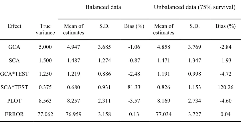
Variance components estimates with SAS PROC MIXED generally agreed with the true values of simulated data. The bias ranged from –4.72% to .13% for all random effects except for SCA by TEST interaction (SCA*TEST, see table 1-1). SCA*TEST has the biggest upward bias (81% for balanced data and 120% for unbalanced data), which may be expected for such a small variance component. The bias increased for all estimates except error variance with imbalance, though this study is not intended to investigate how imbalance would affect accuracy of analysis. For example, bias changed from -1.06% for balanced data sets to -2.84 % at 75% imbalance level for GCA variance, and from -.87% to -1.93% for SCA variance.

(25)

estimate (e.g. for PLOT and ERROR). Data imbalance also increased standard deviation to certain degree.

Table 1-1. Means, standard deviation and percentage bias of estimated variance components for 1000 simulated data sets

Balanced data Unbalanced data (75% survival)

Effect True

variance estimates Mean of S.D. Bias (%) estimates Mean of S.D. Bias (%)

GCA 5.000 4.947 3.685 -1.06 4.858 3.769 -2.84

SCA 1.500 1.487 1.274 -0.87 1.471 1.347 -1.93

GCA*TEST 1.250 1.219 0.886 -2.48 1.191 0.998 -4.72

SCA*TEST 0.375 0.680 0.931 81.33 0.826 1.153 120.26

PLOT 8.563 8.257 2.311 -3.57 8.169 2.734 -4.60

ERROR 77.062 76.959 3.158 0.13 77.034 3.727 0.04

Table 1-2. Mean distances of variance component estimated from true variance and from sample variance of simulated effect values for 1000 simulated data sets

Balanced data Unbalanced data

Effect True variance

components true variance M.D. from sample variance M.D. from M.D. from true variance sample variance M.D. from

GCA 5.000 2.968 1.596 2.976 1.695

SCA 1.500 1.015 0.893 1.083 1.000

GCA*TEST 1.250 0.720 0.672 0.808 0.759

SCA*TEST 0.375 0.680 0.682 0.827 0.826

PLOT 8.563 1.858 1.780 2.229 2.137

ERROR 77.062 2.557 1.160 2.974 2.025

(26)

Similar to standard deviation, mean distances of variance estimates from either true variance or sample variance of true random effects (true sample variance, as defined and discussed in chapter 2) were listed in table 1-2. The size of mean distance varied with true variance and degrees of freedom (Table 1-2). Overall, its range was from .680 to 2.976. For each random effect, a larger mean distance was observed in unbalanced data than in balanced data. Finally, the mean distance from true sample variance was noticeably smaller than that from true variance for GCA and ERROR.

Correlation between true GCA, SCA and BV and their BLUP predictions

The mean correlation of true genetic value and BLUP prediction was high and very close to .9 for both general combining ability (GCA) and breeding value (GV), and lower (around .6) for specific combining ability (SCA) (see table 1-3).

Standard deviation was small for correlation of both GCA and GV, while a bit higher standard deviation was observed for correlation of SCA. Compared with balanced data, mean correlation for both GCA and GV was lower in unbalanced data. Imbalance also increased standard deviation for both SCA and GV.

Table 1-3. Mean correlation and standard deviation of true and predicted GCA, SCA and GV (BLUP) for 1000 simulated data sets

Balanced data Unbalanced data

Effect Mean correlation S.D. Mean correlation S.D.

GCA 0.896 0.115 0.896 0.109

SCA 0.606 0.161 0.587 0.167

GV 0.897 0.086 0.885 0.100

(27)

Comparison with GAREML and DIALL

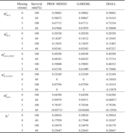
The variance estimates from SAS PROC MIXED, GAREML and DIALL programs were compared (table 1-4). With the balanced data, all three methods produce the exact same estimates of variance components.

Only trivial differences were observed between PROC MIXED and GAREML estimates for three unbalanced data set. Under certain circumstances (e.g. more severe imbalance), slight differences can be observed especially for those estimates close to zero (e.g. SCA, G×E effects), due to the different computing algorithm and iteration criteria of two procedures.

(28)

Table 1-4. Comparison of variance components and individual heritability estimated by SAS PROC MIXED, GAREML and DIALL, with different degree

of balance.

Missing crosses

Survival rate(%)

PROC MIXED GAREML DIALL

(29)

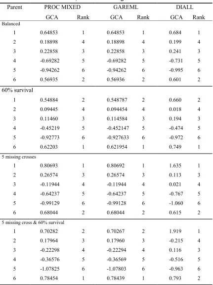
Table 1-5. Comparison of GCA estimated by SAS PROC MIXED, GAREML and DIALL, with different degree of imbalance.

Parent PROC MIXED GAREML DIALL GCA Rank GCA Rank GCA Rank

Balanced

1 0.64853 1 0.64853 1 0.684 1

2 0.18898 4 0.18898 4 0.199 4

3 0.22858 3 0.22858 3 0.241 3

4 -0.69282 5 -0.69282 5 -0.731 5

5 -0.94262 6 -0.94262 6 -0.995 6

6 0.56935 2 0.56936 2 0.601 2

60% survival

1 0.54884 2 0.548787 2 0.660 2

2 0.09445 4 0.094454 4 0.018 4

3 0.11460 3 0.114584 3 0.194 3

4 -0.45219 5 -0.452147 5 -0.474 5

5 -0.92773 6 -0.927633 6 -0.972 6

6 0.62203 1 0.621954 1 0.749 1

5 missing crosses

1 0.80693 1 0.80692 1 1.635 1

2 0.26574 3 0.26574 3 0.113 3

3 -0.11944 4 -0.11944 4 0.021 4

4 -0.64237 5 -0.64237 5 -0.767 5

5 -0.99129 6 -0.99128 6 -1.060 6

6 0.68044 2 0.68044 2 0.615 2

5 missing cross & 60% survival

1 0.70282 2 0.70267 2 1.919 1

2 0.17964 3 0.17960 3 -0.215 4

3 -0.22298 4 -0.22294 4 0.116 3

4 -0.36576 5 -0.36569 5 -0.516 5

5 -1.07825 6 -1.07803 6 -0.963 6

(30)

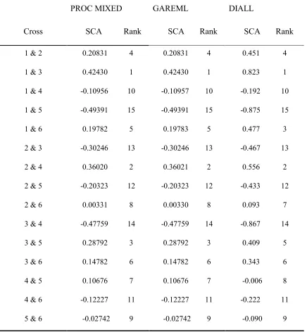
Table 1-6. Comparison of SCA estimated by SAS PROC MIXED, GAREML and DIALL for the balanced data set.

Cross SCA Rank SCA Rank SCA Rank

1 & 2 0.20831 4 0.20831 4 0.451 4

1 & 3 0.42430 1 0.42430 1 0.823 1

1 & 4 -0.10956 10 -0.10957 10 -0.192 10

1 & 5 -0.49391 15 -0.49391 15 -0.875 15

1 & 6 0.19782 5 0.19783 5 0.477 3

2 & 3 -0.30246 13 -0.30246 13 -0.467 13

2 & 4 0.36020 2 0.36021 2 0.556 2

2 & 5 -0.20323 12 -0.20323 12 -0.433 12

2 & 6 0.00331 8 0.00330 8 0.093 7

3 & 4 -0.47759 14 -0.47759 14 -0.867 14

3 & 5 0.28792 3 0.28792 3 0.409 5

3 & 6 0.14782 6 0.14782 6 0.343 6

4 & 5 0.10676 7 0.10676 7 -0.006 8

4 & 6 -0.12227 11 -0.12227 11 -0.222 11

(31)

Table 1-7. Comparison of SCA estimated by SAS PROC MIXED, GAREML and DIALL, for the unbalanced data set with 5 missing crosses and 60% survival

Cross GCA Rank GCA Rank GCA Rank

1 & 2 0.02506 3 0.02508 3 -0.091 7

1 & 3 - - -

1 & 4 - - -

1 & 5 - - -

1 & 6 0.01037 5 0.01038 5 -0.726 10

2 & 3 -0.03848 8 -0.03850 8 -0.047 6

2 & 4 0.06740 2 0.06744 2 1.026 1

2 & 5 -0.04492 9 -0.04495 9 0.051 4

2 & 6 - - -

3 & 4 -0.06740 10 -0.06623 10 -0.525 9

3 & 5 - - -

3 & 6 0.09344 1 0.09349 1 0.493 2

4 & 5 0.01759 4 0.01760 4 0.036 5

4 & 6 -0.03723 7 -0.03725 7 0.140 3

(32)

Discussion

The SAS PROC MIXED procedure can be modified to analyze genetic data from a half-diallel mating design. A dummy variable approach was used to overcome the technical problem presented by the unique feature of diallel designs. The mixed model framework produces all needed genetic parameter estimates and predictions for GCA and SCA.

Through simulation, we have shown that this new procedure can provide accurate variance component estimates for all random variables as compared with the true vales. Since REML does not allow negative estimates of variance components and sets negative estimates to zero, for a small true variance, upward bias is observed and expected. In this simulation study, SCA*TEST only accounts for 0.375% of the total variance and is seriously biased (Table 1-1). Fortunately, for most breeding programs, this effect is only of trivial interest and even eliminated from the model to reduce computational complexity (Lu et al, 1999). For other variance components, REML estimates tend to under estimate the true value due to the upper bias for SCA*TEST, but the biases are small (less than 5% for all). The bias increases with unbalanced data sets. Overall, these results are typical for REML estimates.

Correlations between true genetic values and BLUP estimates are high. Considering the small number of parents of 6, correlation for GCA and BV is high for both balanced and unbalanced data. Small standard deviation for correlation of both GCA and GV indicated that consistently high correlations were achieved in majority of simulated data sets. Lower correlation with larger standard deviation for SCA is expected because of low dominance variance. Although the mating design and field design may not be the best for variance component estimates, the relatively accurate estimates and high correlations with true value for GCA, SCA and GV predictions should be reliable for ranking family and selection.

(33)

estimates (DIALL) becomes distinct. The REML estimator was shown to be superior to the ANOVA based estimator in simulation studies (Swallow and Monahan 1984; Searle et al. 1992; Huber, 1993).

Compared with GAREML and DIALL, one of the advantages offered by the SAS MIXED procedure is that it can be used with model fitting technologies (ML and MIVQUE0) and modified by changing the starting point of iteration, maximum number of iterations and convergence criteria etc. With any degree of imbalance in the data, the SAS PROC MIXED should have better estimates because it uses MIVQUE0 estimators as starting point of iteration and has either stricter default convergence criteria. In fact, when differences do exist, –2 REML log likelihood statistics for GAREML estimates, which can be calculated in PROC MIXED by inputting variance components from GAREML estimates, are slightly larger than those from SAS PROC MIXED. The detailed information about SAS PROC MIXED is described in SAS/STAT system manuals and related publications (SAS Inst. Inc., 1996; Littell et al, 1996).

DIALL calculates general least square solutions (GLS) of genetic effects by treating them as fixed effects and adding sum-to-zero restriction, while PROC MIXED and GAREML provide a consistent treatment of GCA’s and SCA’s as random effects and produce their best linear unbiased predictions (BLUP) (Huber, 1992). The desirable properties of BLUP include maximizing the probability of obtaining correct parental rankings from the data and minimizing the error associated with using the parental values obtained in future applications (Huber, 1993; White and Hodge, 1988). BLUP methodology is particularly more desirable when data are unbalanced and absolute gain assessment is needed.

(34)

estimates. PROC MIXED will also provide other useful information in its outputs. In addition, this practical procedure can be modified to estimate ordinary least square (OLS) or generalized least square (GLS) solutions for GCA and SCA to save computing time. It also provides a friendly interface and many other flexible options compared with other specific packages.

Another useful application is to predict individual tree breeding values using the formula derived in this paper. Usually, within family heritability and within family deviation (i.e.

ijklm

Y -Y_..kl.) are used to calculate within family breeding values. The advantage of formula (8) is that Aˆ _w has desirable properties of BLUP and is particularly more appropriate with unbalanced data. All the information that is needed for calculation can be obtained from PROC MIXED. By first using PROC MIXED to output variance component estimates, inverse of variance matrix and BLUE of fixed effects, we can easily predict individual tree breeding values using IML once again.

(35)

Reference

[1] Borralho, N.M.G. 1995. The impact of individual tree mixed models (BLUP) in tree breeding strategies. In: Eucalypt plantations: improving fibre yield and quality. Proceedings of CRCTHF-IUFRO Conference. Hobart, Australia. p141-145.

[2] Dean, C.A. and Correll, R.L. Analysis of diallel matings with missing values. Silvae Genetica 37(5-6):187-197. 1988.

[3] Huber, D.A. et al, Ordinary least squares estimation of general and specific combining abilities from half-diallel mating designs. Silvae Genetica 41(4-5): 263-273

1992.

[4] Huber, D.A. Optimal mating designs and optimal tehcniques for analysis of quantitative traits in forest genetics. Ph. D. dissertation. University of Florida. 1993

[5] Li, B., McKeand, S.E., Hatcher, A.V., and Weir, R.J. Genetic gains of second generation selections from the NCSU-Industry Cooperative Tree Improvement Program. Pro. 24th South. For. Tree Impr. Conf., p. 234-238. Orlando, Florida, June 9-12, 1997. [1] Li, B., McKeand, S.E., and Weir, R.J. Genetic parameter estimates and selection efficiency for the loblolly pine breeding in the south-eastern US. p. 164-68. In: Tree improvement for sustainable tropical forestry. Proceedings of QFRI-IUFRO Conference. Caloundra, Queensland, Australia. 1996.

[6] Littell, R.C. et al. SAS system for mixed models. SAS Institute Inc. Cary, NC. 1996

[7] Lu, P.X., Huber, D.A., and White, T.L. Potential biases of incomplete linear models in heritability estimation and breeding value prediction. Can. J. For. Res. 29: 724-736. 1999.

[8] SAS Institute Inc. SAS/STAT Software: Changes and enhancements (through release 6.11). Cary, NC. 1996.

[9] Schaffer, H.G. & Usanis, R.A. General least square analysis of diallel experiments. A computer program DIALL. N.C. State Univ., Genet. Dept., Res., Rep. 1. 1969.

(36)

[11]Swallow, W.H. and Monahan, J.F. Monte Carlo comparison of ANOVA, MIVQUE, REML and ML estimators of variance components. Technometrics 26(1): 47-57. 1984.

[12]White T. L. and Hodge, G. R. Best linear prediction of breeding values in a forest tree improvement program. Theor. Appl. Genet. 76:719-727. 1988.

[13]Yanchuk, A. D. General and specific combining ability from disconnected partial diallels of coastal douglas-fir. Silvae Genetica 45(1):37-45 1996.

(37)

Chapter 2 Optimal analytical methodology for

disconnected diallel test

Introduction

(38)

I. Comparison of alternative models in analysis of

disconnected half diallel mating design

Abstract

Simulated data generated with known parameters were analyzed using Best Linear Unbiased Prediction (BLUP) methodology to compare three alternative models, which include diallel as fixed (Model 1), random effect (Model 2) or no diallel effect (Model 3). Both Model 1 and Model 3 produced unbiased GCA variance estimate. Model 2 resulted in downward biased estimate of GCA variance component and occasionally produced unrealistically large diallel variance estimate. Model 3 was slightly better than the other two models in accuracy of GCA variance estimates, while the difference in accuracy between Model 1 and Model 2 was rather trivial. The accuracy of BLUP prediction for three models, measured as the correlation between true genetic value and prediction, was very close, with Model 3 slightly better than the other two. Model 3 is preferred under Randomized Complete Block Design (RCBD) and random selection of parents, while the Model 1 performed well overall in both variance component estimation and BLUP. Model 2 is not recommended in most situations because of its undesirable GCA variance estimate.

(39)

Intoduction

(40)

Theoretical background

Let 12 parents represent a random sample from a base population, assuming general combining ability (GCA) effect of any parent distributed as N(0, σ2

g) and specific

combining ability (SCA) of any mating between two parents distributed as N(0, σ2 s).

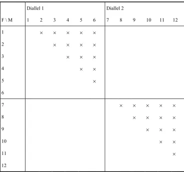
They are randomly assigned into a two 6-parent diallels mating design and are tested under the same environmental condition. Let GCA and SCA be Gi(o) and Sij(o), i, j=1 to 6, o=1,2. From theoretical point of view, there should be no genetic difference other than

random sampling error between the two diallel sets.

If diallel effect Do (o=1,2) is included in the model to assess the random sampling drift of

genetic variance, the assumption of independence of diallel effect and GCA effects Gi(o)

will be violated. In other words, there is no sampling process that leads to a model, which includes an independently identically distributed (iid) nonzero diallel effect and an iid GCA effect. If the genetic diallel effect Do (o=1,2) does exist as NID(0, σ2d), crosses of

the same diallel would have a common genetic effect Do. Then the total genetic value

Do+Gi(o)+Gj(o)+Sij(o) would not be independent within a particular diallel. The covariance

between genetic values of two crosses within the same diallel is σ2

d. On the other hand, if

parents are randomly assigned into 2 diallels, a particular cross will have the same probability of appearing in both diallels. On the population level, the true genetic value of a cross should not change whether it is in diallel 1 or diallel 2. In other words, the diallel or the mating of a set of parents is the result of random sampling, which would not produce any genetic effect.

(41)

On the other hand, if either random selection of parents is violated or some unknown environmental factors are confounded with diallel effect due to flaws in the field experimental design, then elimination of diallel effect will result in an inflated estimate of GCA variance. A complete model with diallel effect may be needed to deal with both situations. However, estimation of an additional parameter (σd2 if treated as random or d if treated as fixed) could potentially affect estimation of other parameters. If diallel is treated as a random effect, it could cause bias in variance estimation using the variance estimation technology REML as in SAS MIXED procedure or GAREML. Since negative variance estimates are not allowed in REML, even if σd2_{=0 the expected value of REML}

estimate of σd2_{is greater than zero. To worsen the situation, two levels of diallel effect}

will give an inaccurate estimate of σd2_{. The variation of this estimate could be fairly}

large.

In this part of the study, we will evaluate the following 3 models using simulation:

1. Complete model with diallel as fixed effect (fixed model or Model 1);

2. Complete model with diallel as random effect (random model or Model 2);

3. Incomplete model with no diallel effect (incomplete model or Model 3).

Simulated data with two and four disconnected diallels will be examimed for all three models.

Method

Linear model

(42)

diallels. Field design is RCBD with 4 tests, 6 blocks and 6 trees per cross per block in each test. The linear model is the following.

Yijoklm = + +µ Ti Bj i( )+Do +Gk o( ) +Gl o( ) +Skl o( ) +TGik o( ) +TGil o( ) +TSikl o( ) +Pijokl+Eijoklm (1)

where,

Yijoklm is the mth observation of the jth block within ith test for the klth cross of the oth

diallel;

µ is the overall mean;

Ti is the fixed effect of ith test, i=1 to 4;

Bj(i) is the fixed effect of jth block within ith test, j=1 to 6;

Do is the oth diallel effect, o=1 to d, random in Model 1, fixed in Model 2, or none in

Model 3;

Gk(o) or Gl(o) is the GCA effect of kth female or lth male of oth diallel (k,l=1, … , 6; k<l) ~

NID(0, σ2 GCA);

Skl(o) is the SCA effect of kth and lth parents of oth diallel ~ NID(0, σ2SCA);

TGik(o) or TGil(o) is the ith test by kth female or lth male GCA of oth diallel interaction ~

NID(0, σ2

TEST*GCA);

TSikl(o) is the ith test by of kth and lth parents SCA of oth diallel interaction ~ NID(0,

σ2

TEST*SCA);

Pijokl is the random effect of plot for the klth cross of oth diallel in the jth block within ith

test ~ NID(0, σ2 PLOT);

Eijoklm is the within plot error term ~ NID(0, σ2E).

Plot means were used in simulation to reduce computational time without affecting results as long as the number of trees per plot are uniform. Plot mean analysis also can deal with imbalance due to missing plots and crosses. Hence the model reduces to the following: ijokl ) o ( ikl ) o ( il ) o ( ik ) o ( kl ) o ( l ) o ( k o ) i ( j i .

ijokl T B D G G S TG TG TS PT

(43)

where, Y_ijokl_.is the plot mean observation of the jth block within ith test for the klth cross of oth diallel;

PTijokl is the random plot mean error for the klth cross of oth diallel in the jth block within

ith test ~ NID(0, σ2

PT), equivalent to Pijokl+ Eijokl.in equation (1) and hence σ2PT=

σ2

PLOT+1/6σ2E;

All other terms are defined the same as in equation (1).

Generation of simulated diallel data sets

Three important parameters are considered in generating diallel data sets: narrow sense heritability, h2; dominance to additive genetic variance ratio, γ; type B genetic correlation, rB. For each parameter, two levels are chosen to represent a higher and lower

value within the normal range of that parameter, resulting in a total of 8 levels of genetic determinations as listed in table 2.1.1.

Without losing generality, the total phenotypic variation is set to be 100. With different parameter combinations, values of σ2

g, σ2s, σ2gt, and σ2st were calculated.σ2p is assumed

to account for 10% of the rest of the variation, thus gives the solutions for σ2

p, σ2e. The

plot mean variance σ2

pt is σ2p+(1/6)σ2e. σ2d is set to zero, as the assumption of random

selection of parents and RCBD field design hold.

Table 2.1.1. Parameter structure for generating simulated data sets

Label h2 γγγγ rB σσσσ2g σσσσ2s σσσσ2gt σσσσ2st σσσσ2p σσσσ2e σσσσ2pt

1 .1 .3 .6 2.500 .750 1.667 .500 9.042 81.374 22.604

2 .1 .3 .8 2.500 .750 .625 .188 9.281 83.531 23.203

3 .1 .7 .6 2.500 1.750 1.667 1.167 8.875 79.874 22.187

4 .1 .7 .8 2.500 1.750 .625 .438 9.156 82.406 22.890

5 .2 .3 .6 5.000 1.500 3.333 1.00 8.083 72.751 20.208

6 .2 .3 .8 5.000 1.500 1.250 .375 8.563 77.062 21.407

7 .2 .7 .6 5.000 3.500 3.333 2.333 7.750 69.751 19.375

(44)

In simulation, test and block effects were generated as random effects, so that each simulated test series has a different set of fixed effects. In the real data, the average test-to -test variation is about 80% of phenotypic variance and block within test variation is 10%. Hence, the variance of test and block are set to be 80 and 10, respectively.

SAS IML procedure was used to produce diallel data sets with the above known parameters. More specifically, by using random number generating function RANOR and multiplying by the square root of variance component we obtained a random vector for each random effect. Random deviations from each vector are then summed up according to the linear model to produce the plot mean vector. The random vector for GCA and SCA effects were also outputted from IML so that the exact genetic values of each parent and cross were known.

For parameter combination 2 and 6, which are the most common genetic structures in practical tree breeding, two types of imbalance at plot level were considered: missing crosses and missing plots. Non-uniform plot survival of different tests and crosses were also taken into account. Altogether four levels of imbalance were generated for these two parameter structures (table 2.1.2).

Table 2.1.2. Imbalance levels considered in simulation study

Label Imbalance description

a 20% missing plot

b 5 missing crosses per diallel

c 20% missing plot plus 5 missing crosses per diallel

d 15% missing plot with 1 low survival test and 5 low survival crosses

PROC MIXED analysis

(45)

MODEL statement. For Model 2, a random diallel effect was included in RANDOM statement. No diallel effect was included in either the MODEL or the RANDOM statement for Model 3.

For each model, best linear unbiased prediction of GCA and SCA effect was obtained for each parent and cross by outputting solution of random effects from PROC MIXED. In the complete model (Model 1 and 2), adjusted GCA was also calculated by adding half of diallel effect (random or fixed) to the parental GCA, assuming both parents of each cross contributed equally to the diallel effect. This adjustment will make parents in two diallels more comparable (Huber et al, 1992).

GCAadj=GCA+0.5*d

Genetic value of each full-sib family was then calculated by adding two parental GCA’s and SCA of the cross.

GV=GCAi+GCAj+SCAij

Thus, three sets of variance component estimates and BLUP of GCA and SCA were obtained for each test series.

Criteria of comparison

Several criteria were used to compare these three linear models.

1. Bias of variance component estimate from true population variance and true sample variance;

2. Mean distance of variance component estimates from true population variance and sample variance;

3. Mean square error of variance component estimates from true parameter and sample variance;

4. Correlation between variance component estimates and true sample variances;

5. Mean distance of GCA and breeding value prediction from true genetic values;

6. Correlation between BLUP’s (of GCA or GV) and true genetic values.

(46)

unknown in practical analysis. But it can be calculated in this simulated study since the true values of random effects are known. For example, 12 true GCA values G1,…,G12 are

generated in each run of simulation, the true sample variance Sg2 is just the sample

variance of these 12 values.

11 ) (

12

1

2 .

2

∑

=

− = i

i

g

g g S

For a given random sample of GCA effect, the goal of any variance component estimation method is to estimate this sample variance Sg2. Hence given Sg2, an unbiased

estimator should have the conditional expectation Sg2, which justified its use as the

unbiasness criteria. Moreover, any estimator cannot be better than Sg2 itself (if Sg2 is

known), because errors always exist in any practical analysis. The advantages of using true sample variance are: 1) In a small simulation study, mean of Sg2 may not converge

closely enough to the true population variance. As a result, sampling error rather than analytical method causes the bias for the most part. The use of Sg2 eliminates the bias due

to sampling error; 2) Correlation of Sg2 and variance estimates can be further calculated

(47)

Results and discussion

Variance components estimation

The variance of diallel effect in the random model

Although there were no true diallel effects in simulated data sets, its estimated variance from the RANDOM model (Model 2) was not negligible in all parameter combinations (Table 2.1.3). The distribution of diallel variance estimate was extremely skewed toward the left. As a result, more than half of the estimates fall to zero. But nonzero estimates frequently occurred regardless of the parameter structure.

Table 2.1.3. Summary statistics of σσσσd2 estimate in Model 2 from analysis of

simulated data sets (1000 for each parameter structure and imbalance level), including mean, standard deviation (S.D.), Coefficient of Variation (CV),

minimum (MIN), maximum (MAX) and 75 percentile

Parameter Structure and imbalance level

Mean S. D. CV(%) MIN MAX 75 percentile

1 1.0534 2.3716 225.1 0 17.122 0.8216

2 1.0855 2.4605 226.7 0 23.383 0.9786

3 1.1693 2.6129 223.5 0 20.584 1.0693

4 0.9688 2.3042 237.8 0 21.796 0.7248

5 1.9212 4.4402 231.1 0 37.816 1.3080

6 1.7921 3.9988 223.1 0 30.479 1.4802

7 1.9459 4.4657 229.5 0 31.761 1.6591

8 1.6936 3.8443 227.0 0 32.535 1.1849

2a 0.9172 2.2891 249.6 0 25.1206 0.6007

2b 0.8902 2.1068 236.7 0 20.477 0.7264

2c 1.0435 2.3364 223.9 0 20.21 0.9468

2d 1.0265 2.371 231.0 0 18.346 0.8591

6a 2.0366 4.807 236.0 0 41.564 1.5866

6b 1.8549 4.7692 257.1 0 54.587 1.2971

6c 2.0549 4.5364 220.8 0 38.091 1.7587

6d 1.7835 4.348 243.8 0 35.639 1.2121

(48)

The mean variance was 1.02, accounting for 41% of σg2 for h2=0.1, and 1.89 or 38% of

σg2_{for h}2_{=0.2. The variation of variance estimates was huge with coefficient of variance}

(C.V.) exceeding 220% in all cases. As also listed in Table 2.1.3, 75 percentiles indicate that 25% of estimates were fairly large, which, on average, was at least 34% of σg2_when

h2=0.1 and 29% of σg2_{when h}2_{=0.2. Moreover, in all parameter structures simulation}

occasionally produced extreme estimates, which were 10 times the magnitude of σg2_.

GCA Variance estimates

Bias

Two measures of bias of GCA variance estimates are listed in Table 2.1.4. All values are expressed as the percentage of true values. As we can see, both Model 1 and 3 provided unbiased estimate of σg2_{. Averaged across 16 simulation runs for data sets, the bias was}

less than 0.5% for both models. But the GCA variance estimate from RANDOM model (Model 2) was biased downward consistently over different simulations. The average bias was –6.03% from population variance and –6.37% from true sample variance.

(49)

Table 2.1.4. Percentage bias of σσσσg2 estimate in 3 models from analysis of simulated

data sets (1000 for each parameter structure and imbalance level)

Percentage Bias

PN* From true population variance From true sample variance

MODEL1 MODEL2 MODEL3 MODEL1 MODEL2 MODEL3

1 2.38 -4.53 2.20 2.76 -4.18 2.57

2 -0.12 -6.50 0.48 -0.55 -6.90 0.05

3 0.96 -7.00 1.09 -1.10 -8.87 -0.98

4 -3.95 -10.08 -3.98 -2.58 -9.52 -2.61

5 3.85 -2.75 3.05 2.14 -4.35 1.35

6 1.63 -4.19 1.32 0.60 -5.16 0.29

7 0.35 -7.07 -0.60 0.71 -6.74 -0.25

8 1.91 -4.95 0.75 1.48 -5.40 0.33

2a -2.10 -7.88 1.58 0.48 -6.65 -0.27

2b 2.38 -4.57 1.44 1.54 -5.36 0.60

2c -0.62 -7.57 0.36 0.71 -6.33 0.97

2d 3.37 -3.48 3.35 0.53 -6.13 0.51

6a 0.13 -6.13 0.33 -0.31 -6.54 -0.11

6b -0.98 -7.01 -1.21 -0.28 -6.35 -0.51

6c -0.14 -6.28 0.37 -1.80 -7.85 -1.30

6d -0.39 -6.55 -0.94 0.58 -5.65 0.02

Mean 0.54 -6.03 0.60 0.31 -6.37 0.04

Note: *  parameter structure and imbalance label, see table 2.1.1, 2.1.2

Variance of σˆ2_g and correlation between Sg2 and σˆ2g

In order for variance of estimates to be comparable for different population variances, C.V. (coefficient of variation) instead of variance was used (Table 2.1.5). The correlation between true sample variance Sg2 and variance estimate σˆg2 is also listed in the Table

2.1.5.

(50)

In terms of correlation between Sg2 and σˆ2_g, the correlation in model 3 was the highest i.e.

.02~.05 higher than that of Model 2, which in turn was about .01~.02 higher than that of Model 1.

The effect of parameter structure on variance estimate can be seen here. High heritability increased correlation between Sg2 and σˆg2 from .7064 for h

2_{=.1 to .7470 for h}2_{=.2 when} γ=.3 and rB=.6. Other changes in parameter structure such as low dominance genetic

control and high type B genetic correlation can also reduce variation of variance estimate and increase correlation b between S2g and σˆ2_g.

Table 2.1.5. Coefficient of variation (C.V.) of σσσσ2

g estimate and correlation between

S2g and σσσσ2g estimate in 3 models from analysis of simulated data sets (1000 for

each parameter structure and imbalance level)

C. V. _Corr(S

g2, σˆ2g)

PN*

Model1 Model2 Model3 Model1 Model2 Model3

1 61.42 61.90 57.90 0.7064 0.7160 0.7484

2 56.76 56.70 52.93 0.7553 0.7700 0.8146

3 67.30 68.67 63.80 0.6718 0.6819 0.7108

4 61.71 62.65 58.79 0.7007 0.7164 0.7610

5 57.78 57.95 55.34 0.7470 0.7591 0.7824

6 52.76 52.95 50.55 0.7966 0.8107 0.8412

7 63.84 64.96 60.77 0.6788 0.6897 0.7125

8 59.16 59.42 55.58 0.7265 0.7381 0.7594

2a 59.78 60.69 56.97 0.7456 0.7572 0.7913

2b 55.94 52.23 52.22 0.7461 0.7584 0.7890

2c 59.30 59.64 55.65 0.6970 0.7070 0.7482

2d 55.21 55.04 51.49 0.7235 0.7387 0.7770

6a 55.95 56.07 53.12 0.7738 0.7884 0.8181

6b 55.41 55.33 52.97 0.8006 0.8119 0.8506

6c 56.61 56.74 53.57 0.7475 0.7624 0.8014

6d 54.40 54.02 51.10 0.7650 0.7833 0.8248

4D6 37.01 35.93 33.99 0.7692 0.7986 0.8493

(51)

Mean distance and mean square error

The mean distance (MD) and mean square error (MSE) provide additional measurements of how estimates are scattered around the target value (as shown in table 2.1.6 and 2.1.7). The less MD or MSE is, the better the estimate is.

Table 2.1.6. Mean distance of σσσσ2

g estimate in 3 models from analysis of simulated

data sets (1000 for each parameter structure and imbalance level)

From σg2 From Sg2

PN* MODEL1 MODEL2 MODEL3 MODEL1 MODEL2 MODEL3

1 1.2236 1.1794 1.1514 0.8709 0.8232 0.7781

2 1.1217 1.0763 1.0518 0.7284 0.6808 0.6060

3 1.3354 1.2912 1.2637 0.9904 0.9446 0.8901

4 1.1859 1.1516 1.1290 0.8211 0.7835 0.7222

2a 1.1750 1.1382 1.1124 0.7681 0.7289 0.6783

2b 1.1174 1.0637 1.0289 0.7571 0.7046 0.6430

2c 1.1583 1.1179 1.1064 0.8235 0.7743 0.7187

2d 1.1167 1.0572 1.0488 0.7835 0.7312 0.6658

5 2.3356 2.3393 2.2295 1.5550 1.4579 1.3954

6 2.0845 2.0222 2.0138 1.2347 1.1613 1.0686

7 2.5424 2.4508 2.4050 1.8614 1.7623 1.6702

8 2.3828 2.2735 2.2129 1.6383 1.5392 1.4448

6a 2.2139 2.1393 2.1275 1.3838 1.2944 1.1899

6b 2.1908 2.1173 2.0926 1.2642 1.1882 1.0834

6c 2.2112 2.1412 2.1197 1.4512 1.3867 1.2627

6d 2.1315 2.0473 2.0184 1.3267 1.2255 1.0811

4D6 1.4616 1.3971 1.3654 0.9126 0.8125 0.7094

Both true population variance σg2 _{and true sample variance S}

g2 were used as target

values. MD and MSE calculated from Sg2 are significantly less than those from σg2,

consistently over all parameter structure and imbalance level. The difference in MD calculated from two criteria (Sg2 and σg2) was about .4 for h2=.1 and .8 for h2=.2, which

(52)

decomposed into the part due to sampling drift and the part due to estimation error. The latter can be measured by MSE from true sample variance. The difference in MSE calculated from two target values (Sg2 and σg2) is significant and accounted for about a

half of total MSE from true population variance σg2. Hence about half of total MSE was caused by sampling drift and was removed from comparing criterion. Because of this reduction in MD or MSE, the differences among three models were more distinguishable for criteria based on true sample variance Sg2.

Model 3 had the smallest MD and MSE from Sg2 and σg2. MD and MSE were larger for

both Model 2 and Model 1. Moreover Model 1 had slightly larger MD and MSE than Model 2. These conclusions hold regardless of parameter structures and data imbalance levels. Therefore, judging only by MD and MSE, Model 3 is the best choice, followed by model 2 and model 1.

Similar effects of parameter structure were shown on estimate. Either low dominance variance or low genetic by environmental effect can improve the accuracy of GCA variance estimation. The effect of heritability or σg2_{is not straightforward here because}

both MD and MSE will change when the magnitude of the true parameter σg2_{or sample}

variance Sg2 changes, as shown in the table. The differences in both MD and MSE were

(53)

Table 2.1.7. Mean square error of σσσσ2

g estimate in 3 models from analysis of

simulated data sets (1000 for each parameter structure and imbalance level)

From σg2 From Sg2

PN* MODEL1 MODEL2 MODEL3 MODEL1 MODEL2 MODEL3

1 2.4726 2.1932 2.1893 1.2428 1.0738 0.9668

2 2.0064 1.814 1.766 0.8622 0.7478 0.5941

3 2.8809 2.5772 2.5957 1.5853 1.4138 1.2892

4 2.2035 2.0227 1.9993 1.122 1.0095 0.8415

2a 2.1945 1.9911 1.965 0.9761 0.8599 0.736

2b 2.0450 1.8139 1.7511 0.9089 0.7846 0.6610

2c 2.1668 1.9335 1.9199 1.1145 0.9767 0.8457

2d 2.0367 1.7675 1.7732 0.9687 0.8318 0.7011

5 9.0209 7.9529 8.1363 3.9871 3.4122 3.1544

6 7.1879 6.4704 6.5558 2.6254 2.2816 1.916

7 10.2509 9.227 9.1131 5.5319 4.8872 4.4873

8 9.0767 8.0291 7.8253 4.3014 3.701 3.315

6a 7.8376 7.0140 7.0924 3.1451 2.7382 2.3459

6b 7.5134 6.7357 6.8368 2.6969 2.3632 1.8907

6c 7.9817 7.1604 7.2199 3.5312 3.1185 2.5928

6d 7.3252 6.4707 6.3942 3.0398 2.5528 2.0433

4D6 3.3446 2.9287 2.8458 1.3658 1.0918 0.7947

GCA and GV prediction

Mean distance and mean square error

(54)

While the mean distance and mean square error of full-sib family genetic value (GV) were larger than those of GCA (as shown in table 2.1.9), similar results were found when different models were compared. Diallel effect adjustment resulted in significant improvement in GCA prediction in both Model 1 and Model 2, though less improvement was observed in Model 2. Regardless of parameter structures and imbalance levels, only trivial difference was found in mean distance and mean square error between two adjusted GVs (in Model 1 and Model 2). Both Model 1 and Model 2 had slightly larger mean distance and mean square error in GV prediction than those in Model 3.

The parameter structures used in this study affected GCA or GV predictions in a similar way to GCA variance estimates. Either low dominance genetic control or high type B genetic correlation could improve the accuracy of prediction. Both MD and MSE increased as the true parameter σg2_{or heritability increases. But this should not lead to}

the conclusion that larger σg2_{reduces the precision of prediction because both criteria}

MD and MSE rely on the magnitude of σg2_{. Unlike variance estimate of}_σg2_{, the}