University of Windsor University of Windsor
Scholarship at UWindsor
Scholarship at UWindsor
Electronic Theses and Dissertations Theses, Dissertations, and Major Papers
1-1-2006
A new energy-based method for evaluating the damping
A new energy-based method for evaluating the damping
properties of cable-damper systems.
properties of cable-damper systems.
Xianshu Jiang
University of Windsor
Follow this and additional works at: https://scholar.uwindsor.ca/etd
Recommended Citation Recommended Citation
Jiang, Xianshu, "A new energy-based method for evaluating the damping properties of cable-damper systems." (2006). Electronic Theses and Dissertations. 7144.
https://scholar.uwindsor.ca/etd/7144
A New Energy-Based Method for
Evaluating the Damping Properties of Cable-Damper Systems
by
Xianshu Jiang
A Thesis
Submitted to the Faculty o f Graduate Studies and Research Through Civil and Environmental Engineering in Partial Fulfillment of the Requirements for the Degree of
Master of Applied Science at the
University of Windsor
Windsor, Ontario, Canada
2006
1*1
Library and Archives Canada Published Heritage Branch3 9 5 W ellingt on S tr e e t Ottaw a ON K 1 A 0 N 4 C a n a d a
Bibliotheque et Archives Canada Direction du
Patrimoine de I'edition
3 9 5 , rue Wellington O ttaw a ON K 1 A 0 N 4 C a n a d a
Your file Votre reference ISBN: 978-0-494-42335-6 Our file Notre reference ISBN: 978-0-494-42335-6
NOTICE:
The author has granted a non exclusive license allowing Library and Archives Canada to reproduce, publish, archive, preserve, conserve, communicate to the public by
telecommunication or on the Internet, loan, distribute and sell theses
worldwide, for commercial or non commercial purposes, in microform, paper, electronic and/or any other formats.
AVIS:
L'auteur a accorde une licence non exclusive permettant a la Bibliotheque et Archives Canada de reproduire, publier, archiver,
sauvegarder, conserver, transmettre au public par telecommunication ou par Nntemet, preter, distribuer et vendre des theses partout dans le monde, a des fins commerciales ou autres, sur support microforme, papier, electronique et/ou autres formats.
The author retains copyright ownership and moral rights in this thesis. Neither the thesis nor substantial extracts from it may be printed or otherwise reproduced without the author's permission.
L'auteur conserve la propriete du droit d'auteur et des droits moraux qui protege cette these. Ni la these ni des extraits substantiels de celle-ci ne doivent etre imprimes ou autrement reproduits sans son autorisation.
In compliance with the Canadian Privacy Act some supporting forms may have been removed from this thesis.
While these forms may be included in the document page count,
their removal does not represent
Conformement a la loi canadienne sur la protection de la vie privee, quelques formulaires secondaires ont ete enleves de cette these.
A bstract
External dampers and cross-ties are commonly used to control vibrations of
stay cables on cable-stayed bridges. While dampers contribute directly to the
structural damping of the attached cables, cross-ties mainly help to increase the
stiffness of the connected cable system. The idea of incorporating cross-ties with
dampers has also been attempted in a few recent applications to benefit from their
combined effect.
A new energy-based method is proposed in the current study to evaluate the
damping properties of a cable-damper system. The proposed method overcomes the
weaknesses and limitations in the previous studies; and its validation is verified
through prior work.
Parametric studies are done to investigate the effect of some parameters on
damping properties of a cable-damper system. Also, studies are conducted to
investigate the combined effect of a damper and cross-ties.
The conversion method which links the effect of the external damper in a
cable-damper system to the equivalent Rayleigh damping of a single cable system is
Acknowledgm ents
I wish to acknowledge my supervisor, Dr. Shaohong Cheng, for her
conscientious supervision for this thesis, Dr. Rupp Carriveau for his tremendous
support and invaluable guidance throughout my research. It was such a wonderful
learning experience and I enjoyed working with them. I also wish to thank my thesis
committee, Dr. Nader Zamani and Dr. Barbara Budkowska for their helpful
comments on my thesis. Finally, I wish to thank my wife, Junru Zhao for her help in
Table o f Contents
Abstract... iii
Acknowledgments...iv
List of Figures...vii
List of Tables... ix
Nomenclature... x
CHAPTER 1 Literature Review...1
1.1 Introduction... 1
1.2 Motivations...9
1.3 Objectives... 13
CHAPTER 2 Energy-Based Evaluation of Damping Properties in Cable-Damper System 16 2.1 Introduction... 16
2.2 Energy-Based Damping Evaluation of a Cable-Damper System...19
2.3 Finite Element Model... 21
2.4 Time-History Analysis Approach...25
2.5 Input of Rayleigh Damping in the Finite Element Analysis... 28
2.6 Equivalent Cable Damping Conversion Method...31
CHAPTER 3 Validation of the Energy-Based Damping Evaluation Method...3 5 3.1 Physical Tests... 35
3.2 Validation of the Proposed Finite Element Model and Time-History Analysis Approach...40
3.3 Validation of the Proposed Energy-Based Damping Evaluation M ethod 43 CHAPTER 4 Parametric Study... 46
4.1 Basic Parameters... 46
4.2 Ranges and Combinations of Parameters...47
4.3 Results... 50
CHAPTER 5 Discussion...5 5 5.1 Effects of Non-dimensional Damping Parameter...55
5.2 Effect of Non-Dimensional Cable Bending Parameter...59
5.3 Effect of Damper Location...60
CHAPTER 6 Conclusions and Recommendations... 70
6.1 General Conclusions...70
6.2 Recommendations for Future Research... 72
REFERENCES...74
List o f Figures
Figure 1-1 The Ponte de Normandie in Le Havre, France...1
Figure 1-2 Different Types of Aerodynamically Treated Cable Surface... 4
Figure 1-3 Cross-Tie Configuration of Cape Girardeau Bridge, Missouri, USA... 5
Figure 1-4 Oil Dampers of the Tsurumi Tsubasa Bridge, Japan...5
Figure 1-5 Combined Application of Cross-ties and Damper on Cable-Stayed Bridges...12
Figure 2-1 Kinetic Energy Decay Curves of Different Cable-Damper Systems...18
Figure 2-2 Configuration of a Cable Damper System... 19
Figure 2-3 Numerical Model of the Cable-Damper System Used in the Current Study... 22
Figure 2-4 PIPE59 Element in ANSYS 10.0...22
Figure 2-5 COMBIN14 Element in ANSYS 10.0... 24
Figure 2-6 Finite Element Model for Damper Assembly...24
Figure 2-7 Relationship between Rayleigh Damping Ratio and Frequency...30
Figure 2-8 Finite Element Models for Equivalent Damping Calculation...32
Figure 2-9 Kinetic Decay Sketches for Equivalent Damping Calculation...33
Figure 2-10 Equivalent Rayleigh Damping Calculation Sketch...34
Figure 3-1 Physical Test Setup in Reference [22]...36
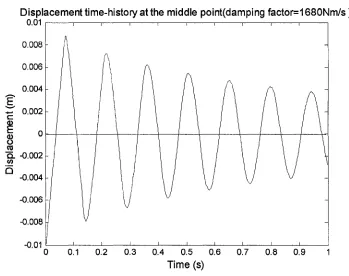
Figure 3-2 Displacement Time-History at the Middle Point(damping factor=1680N ■ m l5)...42
Figure 3-3 Time-History of Kinetic Energy Decay of the Cable-Damper System... 43
Figure 3-4 Finite Element Models used for Validation Analysis...45
Figure 4-1 Time-History of Kinetic Energy Decay Curve (Stiffness^ 14.9 N/m)...54
Figure 5-1 Kinetic Energy Decay Curves (Damper Location Parameter =0.06L)... 56
Figure 5-2 Kinetic Energy Decay Curves (Damper Location Parameter =0.2L)... 56
Figure 5-3 Kinetic Energy Decay Curves (Damper Location Parameter =0.3L)... 57
Figure 5-5 Kinetic Energy Decay Curves (Damper Location Parameter =0.45L)...58
Figure 5-6 Kinetic Energy Decay Curves (Non-Dimensional Cable Bending Stiffness: 100) ...61
Figure 5-7 Kinetic Energy Decay Curves (Non-Dimensional Cable Bending Stiffness: 200) ...62
Figure 5-8 Kinetic Energy Decay Curves (Non-Dimensional Cable Bending Stiffness: 300) ...62
Figure 5-9 Kinetic Energy Decay Curves (Non-Dimensional Cable Bending Stiffness: 400)...63
Figure 5-10 Kinetic Energy Decay Curves (Non-Dimensional Cable Bending Stiffness: 500) ....63
Figure 5-11 Cable Damper Connection... 66
List o f Tables
Table 3 -1 Cable Properties in Reference [22]... ... 36
Table 3 -2 Physical Test Result from Reference [22]... 38
Table 3-4 Comparison of Results...41
Table 3-5 Verification Results...45
Table 4-1 Parameters of the Cable-damper System Used in the Current Study ... 49
Table 4-2 Kinetic Energy Decay Ratio (Damper Location 0.06L)... 51
Table 4-3 Kinetic Energy Decay Ratio (Damper Location 0.2L)... 51
Table 4-4 Kinetic Energy Decay Ratio (Damper Location 0.3L)... 52
Table 4-5 Kinetic Energy Decay Ratio (Damper Location 0.4L)... 52
Table 4-6 Kinetic Energy Decay Ratio (Damper Location 0.45L)... 53
Nom enclature
Sn modal damping for nth mode, [0]
Dn modal dissipated energy per cycle, J, [i7 • Z]
Un modal potential energy, J, \ f • Z]
L total length of the cable, m,
[z]
j kinetic energy decay ration in first vibration second, [0]
maximum kinetic energy of cable-damper system in first vibration period, max
J, [F L\
average kinetic energy of cable-damper system in first one second vibration
period, J, \F L] E ave
x,y,z local coordinate axis in Cartesian system, m,
[z]
F,T damping force or torque, N or Nm, |MZI T 2 j
cv damping coefficient, Nm/s, [mZ2 / Z 3
J
c v i linear damping coefficient in COMBIN14 element, Nm/s, |mZ2/ Z 3]
cv2 second damping coefficient in COMBIN14 element, Nm/s, [ML2 / 7 3 j
T time, s,
[z]
mass matrix
M stiffness matrix
| m| , | m(o| acceleration vector
|« } , |w ( t)| velocity vector
{w }, {//(/)} displacement vector
} external force vector
A diagonal matrix, A = diag(2coi4i)
OJt angular frequency of system, rad/s, [VT\
modal damping ratio, [0]
Q 2 diagonal matrix listing eigenvalues cox ,(o \...(02n , [0]
8 ■ t time step of Newmark integration scheme, s, [7 ]
cc, (5 integration parameters of Newmark integration scheme, [0]
C Rayleigh damping, Nm/s, [ML2 / T 3 j
ct0, ax Rayleigh damping factors, [0]
y/ , Y\ non-dimensional damping parameter, [0]
4 non-dimensional bending stiffness parameter, [0]
EA equivalent axial rigidity of cable, N, [m - L I T 2 J
El equivalent flexural rigidity of cable, Nm2, [m • L3 /7 '2 J
M mass per unit length of cable, Kg, [M]
H axial force acted on cable, N, [/I/ ■ L I T 2\
un cable middle point displacement at nth cycle
un+m cable middle point displacement at (n+m)th cycle
co first undamped angular frequency of cable vibration, rad/s, [l IT]
coD first damped angular frequency of cable vibration, rad/s, [l IT \
Q imaginary part of the eigenvaule
& real part of the eigenvalue
Td damper location parameter, [0]
first mode angular frequency of string equivalent to cable without damper,
® l s
Hz, [lIT]
Ld distance of damper to cable one near end, m, [z]
aQ, a, Rayleigh damping factors, 1/s, [l/7']
c damper coefficient per unit length of cable, N/s, |ML I T 3 j
k' lateral support stiffness per unit length of cable, N/m2, |M !{T2L)\
CH APTER 1 Literature Review
1.1 Introduction
The cable-stayed bridge is a modem type of bridge. It became popular during
the 1950's. Over the last three decades, the cable-stayed bridge has gained increasing
popularity due to its economic advantages and spectacular aesthetic qualities.
Recently, due to advances in materials, design and construction technologies, bridge
spans have become longer and longer. The current longest span cable-stayed bridge is
the Tatara Bridge in Ehime, Japan. It has a main span of 890m. The second longest,
the Ponte de Normandie in Le Havre, France, spans 856m, as shown in Figure 1-1.
The Sutong Bridge in China, which is designed to span 1088m, is currently under
construction. It is expected to be open to the public in 2009.
Figure 1-1 The Ponte de Normandie in Le Havre, France
As a primary structural member of a cable-stayed bridge, the stay cable plays
internal damping and high flexibility, the bridge stay cable is sensitive to dynamic
excitation. Wind is an important source of external excitation which can cause cable
vibration. Wind-induced cable vibration can be classified into several categories
according to its excitation mechanisms: a) Vortex induced vibration (or Aeolian
oscillation); b) Buffeting due to wind gust; c) Classical galloping (typically observed
in iced cables); d) Wake interference (or wake galloping and resonant buffeting);
e)Parametric excitation; f) Reynolds number drag instability; g) Rain-wind induced
vibration; h) High-speed vortex excitation; and i) Dry inclined galloping [1], The
latter three phenomena are specifically related to inclined bridge stay cables. Hikami
& Shiraish [2] first addressed the issue of rain-wind-induced cable vibration on the
Meiko-Nishi Bridge in Japan. The observed vibration, with amplitude up to two times
the cable diameter and frequency between 1-3 Hz, occurred when moderate rain was
accompanied by wind. The excitation mechanisms of high-speed vortex excitation
and dry inclined galloping are not yet clear, while some others such as
rain-wind-induced vibration are now better understood. Countermeasures have been
adopted to various degrees of success in practice.
Frequent and excessive vibration can result in premature cable, connection
failure and/or breakdown of cable corrosion protection system, which reduces the life
vibration is another important issue. In addition, large amplitude vibration of cables
(on the order of l-2m) has been observed when moderate rain and wind exist [4],
Such larger amplitude vibration will certainly raise public concern about the safety of
the bridge [5],
Two different means have been developed to suppress and prevent cable
vibration: a) The aerodynamic countermeasures, i.e. to improve the aerodynamic
properties of the cable; and b) The mechanical countermeasures, i.e. to increase the
damping o f the cable. Various methods have been proposed to improve cable
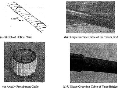
aerodynamic properties. Flamand [6] and Bosdogianni & Olivari [7] proposed to
attach helical wire whirling on the cable surface; Virlogeux [8] suggested adopting
dimpled surface cable; and Saito et al. [9] advised to use axially protuberant cables.
Figure 1-2 shows four types of aerodynamic treatment of the cable surface. Each of
these methods has been proven to be effective and successful to some extent.
Installing cross-ties in the cable plane or attaching an external damper to the cable
near the cable-deck anchorage point are used to increase the damping of the cable
system, which can suppress cable vibration effectively, as shown in Figure 1-3.
Introduction of transverse elements, cross-ties, in the cable plane reduces the free
length o f the crossed cable and thus increases the frequency and stiffness of the cable
vibration [10, 11, and 12]. In general, the behaviour of a cable network is
characterized by an increase of the frequencies with respect to the longest cable.
Installing damping devices on or near the cable-deck anchorage point is also
effective. Figure 1-4 shows an oil damper installed near the deck-anchorage point.
There are three types of external damper available: passive, active and semi-active.
Since cable vibration is often dominated by resonance, very good efficiency can often
be achieved by suitable tuning of a passive damper [13].
0.6 ra
(a) Sketch of Helical Wire (b) Dimple Surface Cable of the Tatara Bridg
M M ili
V . / u k r(c) Axially Protuberant Cable (d) U Shape Grooving Cable of Yuge Bridge
Figure 1-3 Cross-Tie Configuration o f Cape Girardeau Bridge, Missouri, USA
Figure 1 -4 Oil Dampers o f the Tsurumi Tsubasa Bridge, Japan
In the last three decades, much research has been carried out to investigate the
effects of different types of external dampers on suppressing cable vibration through
physical experiments. Using scaled model cables, Xu et al. [14] studied the effects of
an oil damper on cable vibration mitigation. The relationship between the increase of
the cable modal damping ratio and the damper coefficient was investigated through
magnetorheological (MR) damper to cable vibration. Based on the results, the MR
damper was recommended for controlling both free and forced vibration. Gu and Du
[16] successfully reproduced rain-wind-induced cable vibration in a wind tunnel.
They examined the effect of cable inclination angle, cable frequency and cable
damping on cable response.
Generally speaking, experimental tests are expensive. Such tests are
commonly used to verify analytical theories and methods. Analytical methods are
sometimes more useful to help people understand the vibration mechanisms, and
more researchers have devoted their efforts to analytical methods. For example, by
using an analytical/numerical hybrid method, Y.L. Xu et al. [17] explored forced
vibration of sagged cables with discrete oil dampers under harmonic excitation.
Kyu-Sik Park et al. [18] studied the effect of a hybrid control system (lead rubber
bearing and hydraulic actuator or magnetorheological fluid damper) on reducing the
structural response by numerical simulation. Kovacs et al. [19] studied the effect of
viscous-friction dampers and found that they were also effective in increasing system
damping. Further, the installation of a Tuned Mass Damper (TMD) on the vertical
hanger of an arch bridge was also proven to be effective [20], It is very difficult to
cost on different types of dampers. Some representative analytical methods are
reviewed below:
For the vibration of a taut cable with a concentrated viscous damper, S. Krenk
[21] derived a partial differential equation to describe linear oscillations of a cable
under the assumption of a virtually unchanged cable force. The solution was
expressed in terms of damped complex-valued modes. This leads to a transcendental
equation of complex eigenfrequencies. A simple iterative solution to the frequency
equation for all complex eigenfrequencies was proposed. A damping ratio of the
vibration modes, determined from the argument of the complex eigenfrequency, was
derived with high accuracy in two iterations. An accurate asymptotic approximation
of the damping ratio of the low mode was given. Depending on its damping
parameter, the formula allowed for explicit determination of the optimal location of
the viscous damper. In S. Krenk’s work, the cable was considered as a string, thus its
bending stiffness was ignored.
However, the work by Tabatabai & Mehrabi [22] showed that the cable
bending stiffness is an important parameter and should not be neglected. They
proposed a governing differential equation for the vibration of cables with a
parameter of cable flexural stiffness. The equation was then converted to a complex
equation can be solved using many commercial software packages, such as MATLAB
and MathCAD. The estimated values using the method presented were verified by the
results from laboratory testing on a scaled cable model. A parametric study was
conducted for a wide range of non-dimensional parameters. Among the parameters
associated with most stay cables, the influence of cable sag is relatively small,
whereas the cable flexural stiffness can have a significant impact on the resulting
cable damping ratio. In both S. Krenk and Tabatabai & Mehrabi’s research, the
damper has to be located near the cable-deck anchorage point. The distance between
the anchorage point and the external damper location is restricted to be within 6% of
cable length. This is due to the analytical assumption made in simplifying the
governing differential equation.
In the study by J.A. Main and N.P. Jones [23], the damper can be placed at
any location along the cable. The free vibration of a taut cable with an attached linear
viscous damper was explored using an analytical formulation of a complex
eigenvaule problem. They derived an expression for the eigenvalues, which was
independent of the damper coefficient. With the expression, for a given damper, the
modal damping ratio and the corresponding oscillation frequency of each mode can
Some researchers have attempted to explore the damping problem with an
energy-based method. According to the energy-based definition o f the damping ratio
[24], the modal damping, Sn, for the nth mode can be evaluated as the ratio between
the modal dissipated energy per cycle, Dn, and the modal potential energy, Un, i.e.
6m=DJ 4 n Un
(1-1)
Yamaguchi et al. [25] studied modal damping o f structural cables with and
without damping treatment. Modal damping, based on the energy definition, was
derived in the form o f the product of the modal strain energy ratio and the loss factor.
The loss factor is one of the damping parameters and is defined as the ratio of the
dynamically dissipated energy to the strain energy stored per cycle [26], Using the
finite element method, the ratio of modal strain energy to the total potential energy
associated with modal vibration is calculated for both axial and bending
deformations. It has been found that a very large contribution of initial cable stress to
the total potential energy causes a very small strain energy ratio and lower modal
damping in the structural cables.
1.2 Motivations
Some researchers have tried to solve problems related to the cable-damper
differential equation first, then made some simplifications based on the assumption
that the vibration shape of the cable can be represented by its first mode shape, i.e. a
half sine wave. This assumption is reasonable and valid when the damper is located
very close to the cable-deck anchorage, typically less than 6% of the cable length.
The magnitude of the first modal damping of the cable-damper system can be solved
from the simplified governing differential equation.
Another way to calculate the first modal damping of a cable-damper system is
by the logarithmic decrement method. Since the first mode shape of a cable can be
assumed to be a half sine wave when the damper location relative to the cable end is
less than 6% of cable length, the cable-damper system can be considered as a single
degree o f freedom system with the displacement at cable midpoint as the general
coordinate. Thus once a perturbation is introduced, either force or displacement, at
the cable middle point, then the cable is suddenly released, the cable will start to
vibrate freely. The displacement time-history of the cable middle point can be
recorded. This process can be done by physical tests or numerical simulations. Based
on the displacement time-history of the cable middle point, the first modal damping
o f the cable-damper system can be obtained by using the logarithmic decrement
method. However, this approach has a similar limitation like the analytical method in
of the cable vibration shape being a half sine is valid. However, in a cable-damper
system, the shape o f cable vibration will be a combination of several mode shapes
when the damper location to the cable end is beyond 6% of cable length. Moreover,
even when the damper is installed within 6% of cable length to the cable end, its
effect on reducing the amplitude of cable vibration at the damper location will be
significant if the damping coefficient of the damper is relatively large. Consider an
extreme case, of which an external damper is installed at 4% of cable length from the
cable end, with the cable being fixed at both ends and has a total length of L. If the
damping coefficient of the external damper is infinitively large, vibration o f the cable
in the cable-damper plane will not be allowed at the damper location. This is
equivalent to adding an additional rigid constraint to the cable at this location, and the
original cable is broken down into two parts, with lengths being 0.04L and 0.96L,
respectively. Thus, the vibration shape of such a system cannot be represented by a
pure half sine wave.
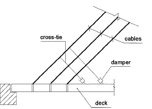
Moreover, a new idea of incorporating cross-ties with dampers has also been
attempted in a few recent applications, as illustrated in Figure 1-5. The cross-ties can
increase the stiffness of the cable network, while the damper can contribute to the
system damping. However, there is no method available to study the combined effect
cross-tie cables
damper
deck
Figure 1-5 Combined Application o f Cross-ties and Damper on Cable-Stayed Bridges
In summary, when considering the combined effect of cross-ties and damper,
or the location of the damper is not very close to the cable-deck anchorage, typically,
beyond 6% of cable length, or its damping coefficient is relatively large, which has
been encountered in practical application, either the analytical method or the
logarithmic decrement method will no longer be valid. So, it is necessary to develop a
new method which is more general, and is capable of handling more practical
scenarios. To eliminate the difficulties that exist in the conventional methods, the new
approach should not be based on the assumption that the vibration shape o f a
cable-damper system can be simply represented by a half sine wave. One possible
way to circumvent these challenges is through the use of the energy method, which
Yamaguchi et al. [25] studied the damping property of a single cable by the
energy method, with the focus on the internal damping of the cable itself Very
limited research has been done to study the damping property o f a cable-damper
system using the energy method. In this study, a new energy-based approach will be
proposed to study the damping of a cable-damper system. The relation between the
kinetic energy decay ratio of the system and its damping property will be
investigated. In the proposed method, there are no restrictions in terms of the location
and the damping coefficient of the external damper. Further, by considering damper
stiffness in the formulation, it is possible to consider the combined effect of cross-ties
and external dampers. A parametric study will be carried out for the following
non-dimensional parameters to examine their impact on the damping property o f the
whole system: a) external damper position; b) non-dimensional cable bending
stiffness parameter; and c) non-dimensional damping parameter. Finally, a method to
convert the kinetic energy decay ratio in a cable-damper system to the equivalent
Rayleigh damping of a single cable will be proposed, which should be of significant
interest to bridge design engineers.
1.3 Objectives
1) To derive an energy-based method for the determination o f damping of a
cable-damper system. For a given cable-damper system, the magnitude of
damping would affect decay rate of cable vibration. In other words, it would
influence how fast the kinetic energy in the system is dissipated. Therefore, the
damping property o f a cable-damper system can be related to the decay rate of
system kinetic energy.
2) To derive a finite element based numerical model for a cable-damper system. The
finite element model will be developed using the commercial software ANSYS.
3) To verify the proposed energy-based method and numerical model. The simulated
cable response will be compared with the results obtained from an earlier physical
experiment.
4) To carry out a parametric study. A verified time-history analysis will be used to
calculate the cable-damper system kinetic energy decay ratio with a combination
of different parameters, i.e. external damper position, non-dimensional cable
bending stiffness parameter, and non-dimensional damping parameter.
5) To derive a method which can convert the decay ratio of kinetic energy in a
cable-damper system to the equivalent Rayleigh damping of a single cable. By
doing so, it will be possible to link the damping effect provided by an external
6) To perform case studies to explore the effect of damper stiffness on cable
vibration. When the damper is installed along cross-ties, the effect of cross-ties
CH APTER 2 Energy-Based Evaluation o f D am ping Properties in Cable-Dam per System
2.1 Introduction
System vibration will only decay in the presence of damping, and the decay of
system kinetic energy is also dependent on damping. How fast the system kinetic
energy will decay depends on how much damping exists in the system. In other
words, the decay rate of system kinetic energy can be interpreted as the system
damping. In this study, the decay rate of kinetic energy o f a cable-damper system is
defined by Eq. (2-1) as follows:
max
where E mrm is the maximum kinetic energy of the cable-damper system, and E ave
is the average kinetic energy of the system within a certain time period, i.e.
where AT is the selected time duration for calculating E ave.
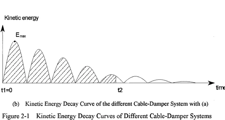
Figures 2-1 (a) and (b) show the kinetic energy decay curves for two different
cable-damper systems. The maximum kinetic energy, Emsx, which occurs in the first
vibration cycle is assumed to be same for these two cable-damper systems. The
time duration of ( t 2 - t x). A FORTRAN program [30] to calculate the total kinetic
energy o f the system within certain time period is written based on Newton-Cotes
formula [35],
Referring to the definition of given by Eq. (2-2), it can be seen that for
the same cable-damper system, the longer the selected time duration {t2 - t x) is, the
less the magnitude of the average kinetic energy E ave will be. It can be inferred that if
the selected time duration approaches to infinity, the average kinetic energy o f the
system will approach to zero and consequently the variation of d in Eq.(2-1) will
close to 1.0 for any cable-damper systems. Thus, the kinetic energy decay ratio
cannot be used as an index o f damping properties of the cable-damper system.
Kinetic energy
t1=0
Kinetic energy
time
t1=0 t2
(b) Kinetic Energy Decay Curve o f the different Cable-Damper System with (a)
Figure 2-1 Kinetic Energy Decay Curves o f Different Cable-Damper Systems
In Figures 2-1 (a) and (b), it can also be seen that if two cable-damper systems
have different damping properties, they will have different kinetic energy decay ratios
within the same time duration. The larger the damping property o f the cable-damper
system has, the faster the kinetic energy will decay. This relationship is valid for any
selected time duration.
Theoretically, any time period can be selected to study the kinetic energy
decay ratio of a cable-damper system. However, if the selected time period is too
short, it may introduce large numerical error; whereas if it is too long, the system
kinetic energy decay ratio d will approach one for any cable-damper system, as
explained in the previous sections. A reasonable choice o f the time duration to
calculate E me and d should be related to the dynamic properties o f the system, in
In the current study, the time period is chosen as one second, which can cover
at least six free vibration cycles of the cable-damper system.
2.2 Energy-Based Damping Evaluation of a Cable-Damper System
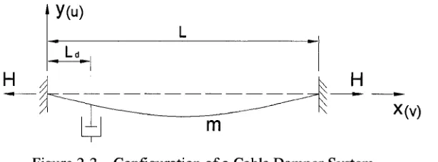
For a typical cable damper system, as shown in Figure 2-2, one possible way
to determine the system kinetic energy is to use an analytical method, i.e. to derive
the governing differential equation, impose the appropriate boundary condition, and
solve it.
H
X(v)
Figure 2-2 Configuration of a Cable Damper System
The governing differential equation of a cable-damper system derived by
Armin B. Mehrabi and Habib Tababain [31] is:
dx2 E l
8 u tt8 2u , d 2y , du d 2u n
- H —- ~ h— t- + k u + c — + m— — = 0
dx dx dt 8t2
(2-3)
where: u is the transverse displacement due to vibration; x is the coordinate along
cable chord; y is the coordinate perpendicular to cable chord; H is the cable force
k' is the lateral spring constant per unit length of the cable; c is the viscous
damping coefficient per unit cable length.; and m is the weight per unit cable length.
Since in the current study, it is assumed that the cable has no lateral support
and sag, so Eq. (2-3) can be simplified as:
d r d 2u ,du d 2u
E l d u
d 2Xj - H — - + cdx dt v m — — — 0dt (2-4) dx
where c = c / L is the damper coefficient per unit length of cable
The boundary conditions for Eq. (2-4) are:
i)A t x = 0: u = 0, — = 0;
dx
* *. . _ du
11) At x = L : u = 0, — = 0;
dx
The solution to Eq. (2-4), can be found analytically, however it requires
tremendous effort.
In the present study, a numerical approach will be used to solve this equation.
A finite element model is developed which contains both cable and damper elements.
Time-history analysis is carried out to simulate the free vibration process of a
cable-damper system. A perturbation (displacement) is introduced at the mid-span of
the cable finite element model and then released suddenly. The responses of the
cable-damper system in terms of nodal displacement, nodal velocity and total kinetic
cable-damper system can be obtained at each time step tx, t2, t3, and so on. The
maximum kinetic energy of the cable-damper system can be easily obtained. The total
kinetic energy within first second divided by one is the average kinetic energy o f the
system free vibration within the first second. Newton-Cotes formula [35] is used to
calculate the total kinetic energy o f the system in first one second and a FORTRAN
program is written for this purpose [30], As a result, the kinetic energy decay rate of a
cable-damper system can be determined. Similar analyses can be carried out for
different parameter combinations. Moreover, a method to convert the kinetic energy
decay ratio of a cable-damper system to the equivalent Rayleigh damping of a single
cable will be proposed, which will be more useful in practical design.
2.3 Finite Element Model
The actual physical cable, as illustrated in Figure 2-2, is fixed at both ends. An
external damper is installed in the transverse direction of the cable. A finite element
model o f the cable-damper system is developed by ANSYS10.0, as shown in Figure
\
dam per
L/2
Perturbation (D isplacem ent)
L
Figure 2-3 Numerical Model of the Cable-Damper System Used in the Current Study
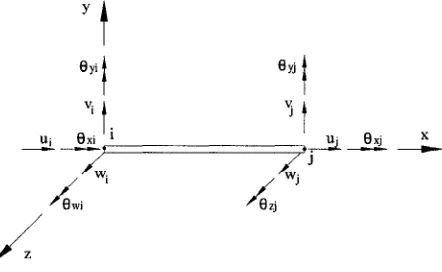
The cable is simulated with the PIPE59 element, which is a uniaxial element
with tension-compression, torsion, and bending capabilities [28], As shown in Figure
2-4, the element has six degrees-of-freedom at each end, i.e., translation in the x, y,
and z direction and rotation about the x, y, and z axis. PIPE59 is similar to general 3D
beam element. In addition, it is capable of simulating stress stiffening effect and large
deflection behaviours. The initial strain in the axial direction can be easily used to
simulate the cable axial force. Other elements, such as BEAM4 in ANSYS, have the
same capabilities as PIPE59. The reason why PIPE59 element is selected in the
current study is due to its simplicity in data input.
0yi
V: V.
The damper is simulated with the C0MBIN14 element. C0MBIN14 can
model longitudinal or torsional deformation in ID, 2D, and 3D applications. The
longitudinal spring-damper option is a uniaxial tension-compression element with up
to three degrees-of-freedom at each end, i.e., translation in the x, y, and z direction.
The longitudinal spring constant should have a unit of “Force/Length”. The unit of
damping coefficient is “Force*Time/Length”. The damping force F or torque T is
computed as:
where cv is the damping coefficient given bycv = cvi +cv2 — ; — is the velocity
dt dt
determined in the previous substep of time-history analysis; cvX is a constant of
linear damping coefficient; and the second damping coefficient cv2 is available to
simulate the non-linear damping effect that needs to be considered in some fluid
environments.
In the present study, the damper is simulated as a ID COMBIN14 element, as
shown in Figure 2-5. The spring or damper property of the element may be removed
from the element. Thus, COMBIN14 element can also be used to simulate a single
C v
-CE-Uj A A A A A A A A A
k
>
U;
Figure 2-5 C0MBIN14 Element in ANSYS 10.0
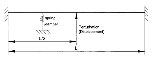
The finite element model presented in Figure 2-3 is used for most analysis
(modal analysis and time-history analysis) in the current study. In order to evaluate
the combined effect of cross-ties and external damper on suppressing cable
vibrations, a more complicated finite element model associated with an external
damper attached to a cable, as shown in Figure 2-6, is used. In this model, two
COMBIN14 elements are used in series. One is used to simulate the behaviour of an
external damper and the other is used to simulate that of the cross-ties. The effect of
cross-tie stiffness in a damper cross-ties assembly can thus be examined.
4 ■
§ spring I
[Xj damper
\ \ \ \ \
L /2
Perturbation (Displacement)
2.4 Time-History Analysis Approach
The equation of equilibrium governing the dynamic response of a structural
system is [27]:
[m |
4+[c]{
4+ m » } = h
1 J 1 J (2-6)
where |M \ is the mass matrix;
[c]
is the damping matrix; [ f ] is the stiffnessmatrix; jw j is the acceleration vector; jw j is the velocity vector; {u} is the
displacement vector, and } is the external force vector.
There are two methods in the ANSYS software, which can be employed for
the linear solution to Eq. (2-6), i.e. the forward difference time integration method
and the Newmark time integration method. The forward difference method is used for
explicit transient analysis and the Newmark method is used for implicit transient
analysis. The Newmark method will be used in the current study. Eq. (2-6) can be
converted to the following form by multiplying the mass orthonormalized
eigenvectors shape (free vibration mode shapes):
j w ( m + a | i # ( 0 j + Q 2 { u{ t ) } = { f * }
where A is a diagonal matrix, A = diag(2a>l^1), <x>l is the i th angular frequency
of system, is the ith modal damping ratio, and Q 2 is a diagonal matrix listing
eigenvalues co2, co\ co2n for the free vibration equation [M ]|w | + W V )= { o }.
A typical row in Eq. (2-7) can be written as:
d 2u ^ du 2 — - + 2 t(o— + a> u = f
d t2 dt J (2-8)
In the Newmark integration scheme, the equilibrium of Eq. (2-8) is considered
at time instant t + d t, i.e.
d 2u
v d t2 j + 2
f d u ^
t+St v dt j t+st
+ co ut+St J t+St
(2-9)
At time instant t + S t, we have
' d u ' \ ' du \
(]I - a)f d 2u '
f ,2 \ d u
+ + a
\ d t ,h+a \ d t ,I V dt 2 y t+a < d*2 yt+St _
a
ut+a ~ ut +l
r d u '
dtJt +
1 Y d lu
V2 ~ PI d ? j
r d 2u^ + f i 2 t V dt Jt+a
a2
(2-10)
(2-11)
where a and j5 are parameters to be chosen to optimize the stability and accuracy
of the solution.
The default values in ANSYS 10.0 for a and are 0.5050 and 0.2525,
respectively, and this will introduce a certain level of numerical damping. If no other
undesirable as high frequencies of the structure can produce unacceptable levels of
numerical noise [29], Newmark proposed the constant average acceleration method as
an unconditional stable scheme, in which case a = 0.5 and ft = 0.25 [27], St is
the increment of the time step, which can be controlled by the input parameter in the
ANSYS software.
Generally, analysis starts from t - 0 , and it is assumed that the initial
conditions of displacement, velocity, and acceleration are known. By combing Eqs.
(2-9)-(2-ll), the displacement, velocity, and acceleration of each node at the next
time step t + St can be obtained. At this point the system kinetic energy can be
calculated. Following the same procedure, the response of the cable-damper system
and system kinetic energy at any subsequent time point can be determined. The
kinetic energy at each time point will be used to calculate the average kinetic energy
of the cable-damper system in the first second. To accelerate the rate of convergence
during time-history analysis, automatic time step technique is used. However, the
maximum time step is kept less than 1/120 of the first vibration period of the
2.5 Input of Rayleigh Damping in the Finite Element Analysis
There are several forms of damping available in the ANSYS software,
including the Rayleigh damping, the material-dependent damping, the constant
material damping coefficient, the constant damping ratio, the modal damping, and the
element damping. The Rayleigh damping and element damping (COMBIN14
element) are used in the current study. The method to input Rayleigh damping
parameters is discussed in the following sections.
It is assumed that the Rayleigh damping is proportional to a combination of
the mass and stiffness matrices, which is given by the sum o f the two alternative
expressions shown in Eq. (2-12).
c = a 0^VT] + a,[A]
(2- 12)
where a0 and a, are constants, they are called Rayleigh damping factors and have
units o f sec-1 and sec, respectively.
Once determined, the parameters a0 and a , , can be input to the ANSYS
software. It is apparent that Rayleigh damping can be converted to the following
relation between the damping ratio and the modal frequency, as shown in Eq. (2-13)
_ a0 | axcon
The two Rayleigh damping factors, a0 and a , , can be evaluated by the
associated with two specific frequencies com and con are known. Writing Eq. (2-13)
for each of these cases and expressing the two equations in the matrix form yields:
When the Rayleigh damping factors are obtained, the proportional damping matrix
that will give the required values of damping ratio at specified frequencies will be
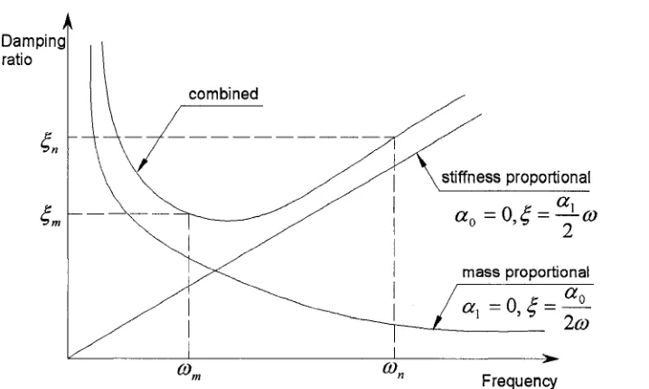
given by the Rayleigh damping according to Eq. (2-12). A simpler method to
formulate the proportional damping is to make it proportional to either mass or the
stiffness matrix, as shown in Figure 2-7. In the figure, the horizontal axis “ co ” is the
circular frequency o f the structure, whereas the vertical axis “ £ ” is the damping ratio. solution of a pair of simultaneous equations if the damping ratios and
(2-14)
The magnitude of Rayleigh damping factors can be expressed as:
Damping ratio
combined
stiffness proportional
m a s s proportional
Frequency
Figure 2-7 Relationship between Rayleigh Damping Ratio and Frequency
In practice, when applying this proportional damping matrix derivation
procedure, it is recommended that com be taken as the fundamental frequency o f the
multiple degree-of-freedom system and con be set among the frequencies of the
higher modes which contribute significantly to the dynamic response. So if (on can
be decided, and then the Rayleigh damping factors can be found.
The higher frequency is decided by the modal coefficient, which is an index of
modal contribution to the dynamic response. Depending on the type of excitation, the
modal coefficient can be computed in five different ways [28], Modal coefficient is
computed for velocity excitation in this study since the energy dissipation depends on
the velocity of cable vibration. The definition of the modal coefficient is given as Eq.
where S V1 is the velocity spectrum of the i th mode, coi is the natural circular
frequency of the i th mode, and y i is the participation factor of the ith mode.
The modal coefficient is a linear function of the velocity spectrum, and the
energy spectrum is a quadratic function of the velocity spectrum. Therefore, the
square of modal coefficient can be used to indicate the modal energy distribution.
When the square of the modal coefficient of a particular mode is less than 4% of the
maximum modal coefficient of the system, the circular frequency of the mode will be
considered as con for determining the Rayleigh damping.
2.6 Equivalent Cable Damping Conversion Method
The present work focuses on studying the variation of d with respect to
different parameter combinations, using the proposed energy-based method. Since
bridge designers are more interested to know the effect of external damper in terms of
equivalent cable damping, a detailed method is proposed in this section to convert the
kinetic energy decay ratio of a cable-damper system to the equivalent Rayleigh
damping of a single cable. To link the effect of an external damper to the equivalent
cable damping, two finite element models are develop, as shown in Figure 2-8. The
damping in this system. Another model is used to simulate the behaviour of a single
cable with Rayleigh damping. The cable bending stiffness parameters are identical in
both models.
Is \
X /
fc
„ Ld
-j d a r t p e r
L L
(a) Cable-damper model (b) Cable alone model
Figure 2-8 Finite Element Models for Equivalent Damping Calculation
As indicated in Figure 2-8(a), for a given damper location, if the
non-dimensional damping parameter has been specified, the kinetic energy decay
ratio of the system can be obtained by the proposed energy-based method. By varying
the magnitude of the non-dimensional damping parameter, its relation with the system
kinetic energy decay ratio at this damper location can be established, as illustrated in
Figure 2-9(a). The curve in Figure 2-9(a) is not the exact curve profile, but is used to
illustrate the conversion method. For a single cable shown in Figure 2-8(b), the
kinetic energy decay ratio could also be obtained through the proposed energy-based
method. If the damping within the cable could be represented by a specific Rayleigh
cable damping property in terms of Rayleigh damping can be established, as shown in
Figure 2-9(b).
damping parameter large
Kinetic energy decay ratio II
s m a
large small
Kinetic energy decay ratio large
Rayleigh damping small
large small
(a) kinetic decay curve of model A (b) kinetic decay curve of model B
Figure 2-9 Kinetic Decay Sketches for Equivalent Damping Calculation
The relation between the damping effect provided by an external damper and
its equivalent Rayleigh damping can be easily developed by integrating information
provided in Figure 2-9.
Here is an example to show the procedure of obtaining equivalent Rayleigh
damping of an external damper with non-dimensional damping parameter y/-, :
Step 1: Draw a horizontal line corresponding to the non-dimensional damping
parameter^, in Figure 2-9 (a), as shown in Figure 2-10 (a).
Step 2: Draw a vertical line in Figure 2-10 (a) from the intersection of the horizontal
kinetic energy decay ratio c>, corresponding to the non-dimensional
damping param eter^,.
Step 3: Draw a horizontal line corresponding to the kinetic energy decay ratio 5X
obtained at step 2 in Figure 2-9 (b), as shown in Figure 2-10(b).
Step 4: Draw a vertical line in Figure 2-10 (b), from the intersection of the
horizontal line obtained at step 3 and the kinetic energy decay curve. Then
find the Rayleigh damping of the cable.
The Rayleigh damping obtained in step 4 has the same capacity to
suppress cable vibration as the external damper with a non-dimensional damping
parameter. Therefore, it is considered to have the equivalent damping to that of the
external damper. Similarly, equivalent Rayleigh damping for external dampers with
other damping properties could be obtained following the same procedure.
damping parameter
large
Kinetic energy d ecay ratio small
large small
Kinetic energy decay ratio large
Rayleigh damping small
large 1
small
(a) (b)
CH A PTER 3 Validation o f the Energy-Based D am ping Evaluation
M ethod
A preliminary analysis is carried out to examine the validity o f the proposed
energy-based method. The validation focused on two aspects: a) verification of the
validity of the proposed finite element model and time-history analysis procedure,
and b) verification o f the concept of the proposed energy-based damping evaluation
method, i.e. an external damper has the same effect to suppress vibration of a
cable-damper system as its equivalent Rayleigh damping does in a single cable.
The validation is based on the experimental work by Tabatabai and Mehrabi
[22], Tabatabai and Mehrabi did physical tests using a representative cable. This
selected “representative” cable is based on the statistical evaluation from a database
of bridge stay cables. And the database was created by Tabatabai et al [33] based on
over 1,400 stay cables from 16 cable-stayed bridges.
3.1 Physical Tests
The setup of the physical test done by Tabatabai and Mehrabi is shown in
Figure 3-1. A representative cable was selected based on statistical information from
a bridge stay cable database. This cable was scaled down by a factor of 6.76, and the
model cable was assembled with the scaled properties calculated on the basis of
diameter strands encased in a polyvinyl chloride pipe. Cement grout was injected in
the encasing pipe based on the common practice in the U.S.A. A tensile force (H) of
122. lkN was applied on the cable. Table 3-1 lists the cable parameters:
Table 3-1 Cable Properties in Reference [22]
Cable length L=13.695m
Equivalent axial rigidity EA=49138 kN (including grout and cover pipe) Equivalent flexural rigidity EI=2.28 kN • m 2 (including grout and cover pipe) Bending stiffness parameter II o o
Mass per unit length m = 3.6kg/m
A viscous damper is attached to the cable at a location of 6% cable length to
one of the cable end. The damper consists of a cylindrical container and a closely fit
moving disk. Oils o f various viscosities were filled in the cylinder to adjust the
damper coefficient.
and the
damper
H
Figure 3-1 Physical Test Setup in Reference [22]
x (v)
Three tests have been carried out on the model, one without damper
coefficient in each case was measured in the laboratory and the response of the
dampers (variation o f force with respect to velocity) was assumed to be linear. For the
two tests conducted with dampers, the damper coefficients were taken as
1680N - s / m and 15130N - s / m , respectively.
In each test, the mid-point of the cable was moved transversely from its
equilibrium position by applying a certain weight, and then released suddenly. The
free vibration response of the first mode at cable mid-point was recorded using an
accelerometer attached to that point. The damping ratio was obtained from the
displacement time-history curve by logarithmic decrement method (free-vibration
decay method) according to the following equation:
In Un = 2n - m S
U n+m (3-1)
where un is the displacement at cable middle point in the n th cycle; un+m is the
displacement at cable middle point displacement in the (n + m)th cycle; co is the
first undamped angular frequency o f cable vibration; coD is the first damped angular
frequency of cable vibration; and 8 is the damping ratio of the cable-damper system.
The experimentally measured and theoretically calculated damping ratios by
Table 3-2 Physical Test Result from Reference [22]
Case number
Damping factor
N ■m i s
Damping parameter ¥ Bending stiffness parameter First frequency (Hz)
Damping ratio associated with damper S (%)
Calculated damping ratios Direct measurement Associated with damper
1 0 0 100 7.028 0.3 0 N/A
2 1680 2.5 100 7.028 2.7 2.4 2.0
3 15130 22.8 100 7.320 1.5 1.2 1.5
The damping ratios obtained from the physical experiment are presented in
two forms. One is the directly measured total damping ratio of the system and the
other is the damping associated with the damper alone. The latter is obtained by
subtracting the damping ratio of the cable without damper from the directly measured
value. In the derivation, it is assumed that the intrinsic damping of the cable (for the
cable without damping) remain constant with the addition of the external damper.
A discrepancy between the experimental and the analytical results can be seen
in Table 3-2. For Case 2, the damping ratio from analysis is lower than that from
experiment. The analytical result is 2.0 whereas the experimental result is 2.4. For
Case 3, the damping ratio from analysis is higher than that from the experiment,
experimental error. Generally speaking, it is possible to determine an appropriate
viscous damping property by experiments. The commonly used experimental
methods for this propose include: the logarithmic decrement method (free-vibration
decay method) [32], the resonant amplification method, the half-power (band-width)
method [34], and the resonance energy loss per cycle method. Among them, the
logarithmic decrement method is the simplest and the most often used one. Tabatabai
and Mehrabi used this method to determine the damping ratio of the system in their
study [22], The main advantage of the logarithmic decrement method is that the
requirement of equipment and instrumentation is minimal. The vibration can be
initiated by any convenient method and only the relative displacement amplitude
needs to be measured. However, the damping ratio obtained by this method is
amplitude dependent. For example, “m” consecutive cycles in the earlier portion of
the high-amplitude free vibration response will yield a different damping ratio than
“m” consecutive cycles in the later stage of a much lower response. It is usually found
that in such a case, the damping ratio decreases with decreasing amplitude of free
vibration response. For the complexity of damping problem, sometimes it is difficult
to obtain an accurate solution of the problem even with very complex and advanced
equipment. Therefore, the logarithmic decrement method is still widely used to make
3.2 Validation of the Proposed Finite Element Model and Time-History
Analysis Approach
Both the modal and time-history analysis are carried out by simulating the
behaviour of the cable model used in the physical tests described in Section 3.1. The
period of the first free vibration of the cable-damper system obtained from the modal
analysis is compared with the physical test results given in reference [22], The
time-history of cable nodal displacement is used to calculate the Rayleigh damping of
the cable-damper system, which is then compared with the previous study results[22].
The same finite element model is used for both the modal and the time-history
analysis. The cable is simulated by the PIPE59 element and the damper is simulated
by one COMB INI 4 element. The input parameters of cable properties and cable
pretension in the finite element model are computed based on the given physical
Table 3-3 Input Parameters Used in the Finite Element Model
Cable property
Elastic modulus (N/m2) 8.489E10
Radius (m) 1.360E-2
Cross sectional area (m2) 5.810E-4
Weight density (kg/m3) 6196.740
Initial strain in the axial direction 2.476E-3
Damper property
Damping coefficient (Nm/s) 1680,15130
Damper stiffness (N/m) 0
Damper location 0.06L
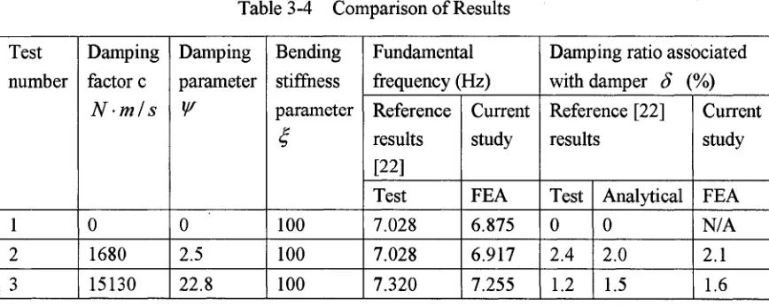
Using the data provided in Table 3-3, both the modal analysis and
time-history analysis are carried out. The modal analysis results are shown in Table
3-4. The analysis results match the experimental results very well and the maximum
error is about 2%.
Two separate time-history analyses are carried out for a damper coefficient of
1680N*m/s and 15130 N*m/s, respectively. The results of damping ratio of the
cable-damper system are given in Table 3-4.
Table 3-4 Comparison of Results
Test number
Damping factor c
N - m l s
Damping parameter ¥ Bending stiffness parameter Fundamental frequency (Hz)
Damping ratio associated with damper S (%) Reference results [22] Current study Reference [22] results Current study
Test FEA Test Analytical FEA
1 0 0 100 7.028 6.875 0 0 N/A
2 1680 2.5 100 7.028 6.917 2.4 2.0 2.1
The displacement time-history o f the cable middle point is illustrated in
Figure 3-2, based on which the system damping can be determined by the logarithmic
decrement method. Figure 3-3 shows the time-history of the kinetic energy decay rate
of the cable-damper system. The system kinetic energy ratio as defined by Eq. (2-1)
can therefore be computed.
Displacem ent time-history at the middle point(damping fac to r= 16 80 N m /s)
0.01
0.008
0.006
0.004
~ 0.002
Q. -0.002
-0.004
-0.006
-0.008
-0.01
0.2 0.3 0.4 0.5 0.6 0.7 0.8 0.9
Tim e (s)
Tim e-history of kinetic energy d ec ay of the c a b le -d a m p e r system
^ 30
0.2 0.3 0.4 0.5 0.6 0.7 0.8
T im e (s)
Figure 3-3 Time-History of Kinetic Energy Decay of the Cable-Damper System
The results in Table 3-4 revealed that the fundamental frequency and the
damping ratio of the cable-damper system simulated by the proposed finite element
model and analyzed by the proposed time-history analysis approach agree reasonably
well with that by Tabatabai et al [22],
3.3 Validation of the Proposed Energy-Based Damping Evaluation Method
In Section 3.2 the validity of the proposed finite element model and the
time-history analysis procedure have been verified. Another series of finite element
energy-based method. The proposed method assumes that the damping provided by
the external damper in a cable-damper system has the same damping effect to
dissipate kinetic energy and suppress cable vibration as the equivalent Rayleigh
damping in a single cable.
Tabatabai and Mehrabi [22] obtained the equivalent Rayleigh damping of a
cable-damper system through physical experiments and numerical simulation. The
cable properties and damper parameters are given in Table 3-1 and Table 3-2,
respectively. These parameters are used in the current study to verify the validity of
the proposed energy-based method. Two finite element models as shown in Figure
3-4 are developed in this study. Model A is a cable-damper system with no Rayleigh
damping in the cable, whereas model B is a single cable with the Rayleigh damping
obtained in the physical tests by Tabatabai and Mehrabi [22], The input of Rayleigh
damping to the finite element model is according to the method discussed in Chapter
2. The properties of the cables in these two models are identical. A transverse
displacement is introduced at the cable middle point and then released suddenly. This
process is simulated numerically by the finite element method. Time-history analysis
is carried out for each model. The kinetic energy decay ratios of the two models are
obtained, which are presented in Table 3-5. Results show that the kinetic energy
kinetic energy decay ratio due to the equivalent Rayleigh damping in Model B. Thus,
the idea of using energy-based method to evaluate the damping property of a
cable-damper system is proved to be valid.
u darrper
Model A: Cable-damper system without B: Single cable with Rayleigh damping Rayleigh damping
Figure 3-4 Finite Element Models used for Validation Analysis
Table 3-5 Verification Results
Kinetic energy decay ratio
Model A Model B
Experiment damping Numerical damping Case I (damper coefficient
1680Nm/s) 0.76 0.80 0.78
Case II (damper coefficient