Material parameter estimation and hypothesis testing on a 1D viscoelastic stenosis model: Methodology

(1)

Material parameter estimation and hypothesis testing on a

1D viscoelastic stenosis model: Methodology

H.T. Banks, Shuhua Hu, and Z.R. Kenz

Center for Research in Scientific Computation Center for Quantitative Sciences in Biomedicine North Carolina State University, Raleigh, NC 27695-8212

Carola Kruse, Simon Shaw, and J.R. Whiteman

BICOM, Brunel University, Uxbridge, UB8 3PH, England

M.P. Brewin and S.E. Greenwald

Blizard Institute, Barts and the London School of Medicine and Dentistry, Queen Mary, University of London, England

M.J. Birch

Clinical Physics, Barts and the London National Health Service Trust, England

April 9, 2012

Abstract

Non-invasive detection, location and characterization of an arterial stenosis (a blockage or partial blockage in the artery) continues to be an important problem in medicine. Partial blockage stenoses are known to generate disturbances in blood flow which generate shear waves in the chest cavity. We examine a one-dimensional viscoelastic model that incorporates Kelvin-Voigt damping and internal variables, and develop a proof-of-concept methodology using simulated data. We first develop an estimation procedure for the material parameters. We use that procedure to determine confidence intervals for the parameters found, which indicates the efficacy of finding parameter estimates in practice. Confidence intervals are computed using asymptotic error theory as well as bootstrapping. We then develop a model comparison test to be used in determining if a particular data set came from a low input amplitude or a high input amplitude, which we anticipate will aid in determining when stenosis is present. These two thrusts together will serve as the methodological basis for our future analysis using experimental data currently being collected.

Mathematics Subject Classification: 62F12; 62F40; 65M32; 74D05.

(2)

1 Introduction

Current methods to detect and locate arterial stenoses (blocked arteries) include somewhat invasive angiography and expensive CT scans. Neither procedure is particularly easy to administer, while the CT scan can localize hard plaques but not soft plaques [Luke]. Accordingly, there is interest in examining other methods to determine the existence and location of stenosed vessels. Previous work [Luke, Sam, BaSam, BaPint, BaMedPint, BaLu, BBETW] focused on developing a sensor device to be used with a physical model of a chest cavity, and then developing a mathematical model to describe the medium in which a stenosis-generated acoustic signal is propagated to the chest surface. After an interregnum of roughly five years between that earlier work and our current efforts, we have returned to the early ideas and have reformulated the problem to some extent. This is motivated by companion experiments being conducted with novel acoustic phantoms built at Queen Mary, University of London (QMUL) and Barts & London NHS Trust (BLT) in England. Our viscoelastic model will be quite general, incorporating Kelvin-Voigt damping and internal variables in a hysteresis formulation, so as to provide maximum flexibility in these early stages of model development and analysis.

In this work, we continue to use mathematical modeling techniques in order to non-invasively determine the existence and location of any arterial stenoses, ideally through sensors placed only on the surface of the chest. To this end, we have developed novel experiments to produce one-dimensional pressure wave data that can be fit using the viscoelastic model developed here. While this work will be informed partly by test experimental devices which have been built, it is important to note that all the data employed in this initial mathematical formulation will be simulated data. Broadly, then, the work here is intended to serve as a proof-of-concept of our mathematical and statistical inverse problem methodology, using simulated data very similar to the experimental data we will subsequently use with these methods along with incorporation of standard viscoelastic models (see, e.g., [BaHuKe]).

(3)

1.1 Problem formulation

X=L

X=0 One-dimensional domain

!"#$%&'(%)*&$"+,-./01&applied

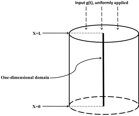
Figure 1: Setup of agar phantom, with sample one-dimensional domain denoted

In this work, we will examine a simplified one-dimensional model for an agar phantom, as pictured in Figure 1. This configuration is an approximation (under certain assumptions) to the novel experimental devices we are using at QMUL to gather experimental data. Development of general viscoelastic equations can be found throughout the literature; in particular, one may refer to [BaHuKe] as a source of the model components discussed in this current work. As in the example in [BaHuKe], we make simplifying assumptions that will result in a one-dimensional wave equation. If we assume a uniform force applied along the top of the phantom and radial symmetry within the phantom (in part to closely match the symmetrically constructed phantoms used at QMUL), then we can simplify the cylindrical physical domain to a one-dimensional domain and to finding the functionu(x, t) which represents the material response to, in this case, an applied stenosis-generated like force.

(4)

we obtain the system for the displacement u

ρutt−σx= 0

u(0, t) = 0, σ(L, t) =−g(t),

u(x,0) = 0, ut(x,0) = 0.

(1)

A constitutive relationship for stress σ(x, t) in terms of strain must be developed. To this end, we assume that the stress is described by a combined model with Kelvin-Voigt damping and Maxwell-Zener internal variables (also known as the generalized standard linear solid model). We begin with the equation

σ =E1uxt+E0

P(0)ux−

Z t

0

Ps(t−s)ux(s)ds

(2)

The Kelvin-Voigt damping is represented by the term involvingE1. The form of the stress relaxation

function P(t) is assumed to be a Prony series

P(t) = p0+

Np

X

j=1

pje−t/τj,

where we assume all the pj are nonnegative numbers and the τj values are positive, and with Np being a positive integer. This series makes the assumption that relaxation in a material can be represented by a discrete number of relaxation times τj. Without loss of generality, we will also

enforce P(0) = 1. A result of this constraint is that

Np

X

j=0

pj = 1. If we replace Ps(t−s) in (2) with

the s-derivative of the Prony series at t−s, we obtain

σ =E1uxt+E0 ux−

Np

X

j=1

Z t

0

pj

τj

e−(t−s)/τj_u

x(s)ds

!

.

We can reformulate the integrals related to each internal variable as differential equations which we can solve simultaneously with the main system PDE. To this end, we define

ǫj ₌

Z t

0

pj

τj

e−(t−s)/τj_u

x(s)ds.

Then the time derivative ofǫj is given by

ǫjt =

pj

τj

ux(t)− 1

τj

Z t

0

pj

τj

e−(t−s)/τj_u

x(s)ds.

Relatingǫj and ǫj_t allows us to model the internal variables dynamically as

τjǫjt+ǫj =pjux,

(5)

for j = 1,2, . . . , Np. Then we can write the overall stress-strain relationship as

σ = E1uxt+E0 ux−

Np

X

j=1

ǫj

!

. (4)

Note that even thoughp0 is an element in the Prony series forP(t), once the series is substituted in

the model the constantp0no longer appears. However,p0is still present in the sum-to-one constraint

on all pi values, but we can easily work with the alternate constraint that the remaining pj terms

follow

Np

X

j=1

pj ≤1. Then, E0 andE1 along with the relaxation times represent the parameters which

affect the response of a particular material to stresses. We incorporate Kelvin-Voigt damping via theE1uxtterm in (4). Development of these models is described in [BaHuKe], as well as in standard viscoelastic theory [FiLaOn, Lak, GoGr, Fer, CoNo, FaMo]. The damping and internal variables provide us the future flexibility to match the model to data from the experimental device, and also present an interesting question of identifiability of the damping and internal variable parameters which we will later discuss in depth. Note also that the authors in [BBETW, Luke, Sam] give computational results (using essentially an equivalent model from a slightly different conceptual formulation involving a distribution of relaxation mechanisms-see [BaPint]) showing that discrete relaxation times can model well the viscoelastic material responses of the type we consider in this work (namely, attempting to mimic the response of biological soft tissue). In fact, in previous work no more than two discrete relaxation times were used, which has informed our decision to allow a maximum of two relaxation times.

Since the ultimate goal of the wider research project will be examining the traction into the chest cavity that results from a healthy artery experiencing a heartbeat as compared with an artery containing a stenosis, our nonzero boundary inputg(t) will here be represented by an approximation to a pulse traction. In order to ensure a smooth, compactly supported input, we implement the input function as a Van Bladel function. This smoothness is useful in order to get the maximum benefit from using high order numerics.

The function used is

g(t) =







A·exp

|ab|

t(t+a−b)

if t∈(0, b−a),

0 otherwise.

(5)

Altogether, this description (1), (3) and (4) along with (5) encompasses the one-dimensional model for the displacement u(x, t) that will be studied in both major sections of this work.

(6)

1.2 Parameter values

We pick values for the system parameters which simulate low-amplitude (on the order of 0.1mm) oscillatory motion, motivated by the experimental data to which we intend to apply this method-ology. For data generation, we will use two internal variables (Np = 2). The weights pi for our two relaxation time model will be as shown below. The baseline material parameter values chosen for this work are as follows:

E0 = 2.2×105 Pa, E1 = 40 Pa·s, ρ= 1010 kg/m3, L= 0.053 m

τ1 = 0.05 s, τ2 = 10 s, p1 = 0.3, p2 = 0.55. (6)

Note that the densityρ= 1010 kg/m3 is the true density of the agar gel that is used in the medium for our experiments at QMUL, and L = 0.053 m is the true height of the phantom. These are parameter values which are directly taken to approximate the experimental device. The values for

E0 and E1 and for the relaxation times are physically reasonable parameters based on a perusal of

the viscoelastic materials research literature and are also informed by our early experiments with the agar gels.

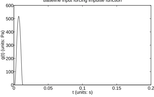
In the Van Bladel function, the values of a and b have an effect on pulse width as well as the amplitude. We takea= 6×10−3 _and_b_{= 20}_×₁₀−3 _{for an effective pulse application time of 14}_ms_.

We then use A to scale the amplitude, in this case taking A = 6×103. The Van Bladel function with these parameter values, which we will use as our “true” input function, is depicted in Figure 2.

0 0.05 0.1 0.15 0.2

0 100 200 300 400 500 600

t (units: s)

g(t) (units: Pa)

Baseline input forcing impulse function

Figure 2: Van Bladel function (5) with A= 6×103, a= 6×10−3_{, and} _b_{= 20}_×₁₀−3_.

In reality, one will obtain a set of experimental data and then one needs to determine how many (if any) relaxation times are required to represent well the data. Thus, we will want to compare the performance of three models. In each model, we will always estimate E0 and E1 (assuming given

(7)

1. For a model with no relaxation times, we do not include any τi or corresponding pi in the model. Thus, we estimate only E0 and E1.

2. In the case with one relaxation time, we incorporate a single internal variable (i.e., Np = 1), corresponding with relaxation time τ1, and use the material weights

p1 = 0.3. (7)

3. For the case of two relaxation times, we will use the material weights in (6), given by

p1 = 0.3, p2 = 0.55. (8)

Considering this set of models will allow us to follow what one would consider in practice, examining the results of adding/subtracting model features. It is worth noting here that for this particular set of models, the one-relaxation-time model (the second case) is not a special case of the two-relaxation-time model (the third case) as the material weighting p2 in the two-relaxation-time model is fixed,

and that the no-time-relaxation-time model (the first case) is not a special case of the one-time-relaxation model as the material weighting p1 in the one-relaxation-time model is fixed. However, if

we allow the corresponding material weights to be free (i.e., to be estimated along with relaxation times), then the no-relaxation-time model is indeed a special case of the one-relaxation-time model, and the one-relaxation-time model is a special case of the two-relaxation-time model. We will use the sensitivity equations and parameter estimation results as well as model selection criteria to suggest the number of relaxation times to use in practice.

1.3 “True” model

Using the baseline parameters, we present a graph of the noiseless model response, what we will henceforth call the “true” system motion in Figure 3. This is the simulated device motion from which we will generate our data, and also demonstrates motion under the true parameter values which we will use with our inverse problem methodology to attempt to recover from noisy data. Note that the motion is on the 1/10 millimeter scale, which was again motivated by the likely scale of results from the experimental device.

2 Estimation of material parameters

(8)

0 0.05 0.1 0.15 0.2 0.25 −2

−1.5 −1 −0.5 0 0.5 1 1.5x 10

−4

t (units: s)

u(L,t) (units: m)

Model solution at true parameters

Figure 3: Solution of model (1), (3) and (4) using the “true” parameters (6) and forcing function with parameters a= 6×10−3_,_b _{= 20}_×₁₀−3_{, and}_A _{= 6}_×₁₀3_.

2.1 Study of effects of changing material parameters

Before discussing simulated data and actually solving the inverse problem, we wish to complete some analysis on the model around the “true” material parameter values (6). It is clear that changing the amplitude factorA for the Van Bladel input will change the resulting amplitude of the system. Hence, we consider here changes in the material parameters E0, E1, and τj values.

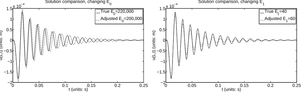
We first consider changes in the stiffness E0 and damping factor E1. As an example of typical

effects of changing parameters, we show the effects of reducing stiffness toE0 = 200,000 in the left

pane of Figure 4 and in the right pane the effects of increasing the damping to E1 = 60. Changes

0 0.05 0.1 0.15 0.2 0.25 −2

−1.5 −1 −0.5 0 0.5 1 1.5x 10

−4

t (units: s)

u(L,t) (units: m)

Solution comparison, changing E

0

True E₀=220,000 Adjusted E

0=200,000

0 0.05 0.1 0.15 0.2 0.25 −2

−1.5 −1 −0.5 0 0.5 1 1.5x 10

−4

t (units: s)

u(L,t) (units: m)

Solution comparison, changing E

1

True E₁=40 Adjusted E

1=60

Figure 4: Solution of model (1), (3) and (4) using the “true” parameters (6) and forcing function with parametersa= 6×10−3_, _b_{= 20}_×₁₀−3_{, and}_A _{= 6}_×₁₀3 _{(depicted by the solid line), alongside}

solutions usingE0 = 2×105 (left pane) andE1 = 60 (right pane) which are represented with dashed

lines in their respective graphs.

(9)

on peak heights. This is known – a more stiff material will propagate waves more quickly and will dissipate energy less slowly. Increases in damping, E1, lead to the expected effects that the

energy dissipates faster in the material, so the oscillation peak heights become smaller and the material experiences fewer small oscillations at later simulation times. As one might expect, these two parameters seem to govern the major properties of how the material responds to an impulse response traction.

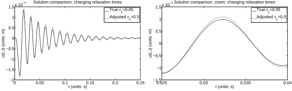
Relaxation times can allow the model flexibility in matching the periodic local “peaks” and “troughs” in the oscillating solution. For example, if we change from the baseline τ1 = 0.05 to

τ1 = 0.5, the system experiences the changes shown in Figure 5. This response to changing relaxation

0 0.05 0.1 0.15 0.2 0.25 −2

−1.5 −1 −0.5 0 0.5 1 1.5x 10

−4

t (units: s)

u(L,t) (units: m)

Solution comparison, changing relaxation times True τ

1=0.05

Adjusted τ

1=0.5

0.025 0.03 0.035 0.04 −1.5

−1 −0.5 0 0.5 1 1.5x 10

−4

t (units: s)

u(L,t) (units: m)

Solution comparison, zoom, changing relaxation times True τ

1=0.05

Adjusted τ

1=0.5

Figure 5: Solution of model (1), (3) and (4) using the “true” parameters (6) and forcing function with parameters a = 6 × 10−3_, _b _{= 20} _×₁₀−3_{, and} _A _{= 6} _×₁₀3 _{(depicted by the solid line),}

alongside the dashed line using τ1 = 0.5 with the remaining parameters the same. The right pane

demonstrates the solution zoomed in fort ∈[0.025,0.04].

times represents a typical example of changing eitherτ1orτ2. However, note the scale of the changes:

the maximum difference between the solutions shown in Figure 5 is 1.0996×10−5_{. As we will see}

later when adding noise, the noise itself is on the scale of 10−5

. This foreshadows the difficulties in properly estimating relaxation times that we will see going forward. This will be evident also both in a discussion on using different optimization routines and in a discussion of model sensitivity with respect to parameters.

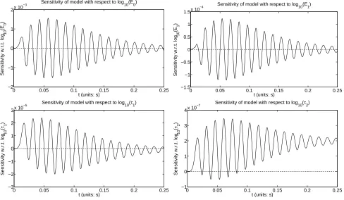
2.2 Sensitivity of model output with respect to material parameters

In order to further quantify the model response to changes in parameters around the baseline values of (6), we will examine the sensitivity of the model output with respect to material parameters. Note that since the values of parameters are on such a varying scale, we will actually work with the log-scaled versions of the material parameters we are attempting to estimate. In other words, if ¯θ = (E0, E1, τ1, τ2)T is the vector of parameters to be estimated, we define θ = log10(¯θ).

(10)

To compute the sensitivity of the model output to each parameter, one needs to find sensitivity equations which describe the time evolution of the partial derivatives of the model state with respect to each parameter. Sensitivity equations in terms of the non-log-scaled parameters ¯θ are derived in Appendix A. Since we are only using observations at the x=L position, we will actually consider only the sensitivities with respect to each parameter at this position.

We can use the sensitivity of model output to the non-log-scaled parameters to find the sensitivity of model output with respect to the log-scaled parameters, which will be of interest here. Using the chain rule, we find that

∂u(L, t; 10θ₎

∂θi

= ¯θiln(10)

∂u(L, t; ¯θ)

∂θ¯i

,

where θi and ¯θi are theith element of θ and ¯θ, respectively.

The sensitivities of model output with respect to parameters (log₁₀(E0),log10(E1),log10(τ1),

log10(τ2)) are shown in Figure 6. From this figure we see that model output is most sensitive to

0 0.05 0.1 0.15 0.2 0.25 −2

−1 0 1 2x 10

−3

t (units: s)

Sensitivity w.r.t. log

10

(E

0

)

Sensitivity of model with respect to log

10(E0)

0 0.05 0.1 0.15 0.2 0.25 −1.5 −1 −0.5 0 0.5 1 1.5x 10

−4

t (units: s)

10

(E

1

)

10(E1)

0 0.05 0.1 0.15 0.2 0.25 −3 −2 −1 0 1 2 3x 10

−5

t (units: s)

10

(

τ1

)

10(τ1)

0 0.05 0.1 0.15 0.2 0.25 −1

0 1 2 3 4x 10

−7

t (units: s)

10

(

τ2

)

10(τ2)

Figure 6: (upper left pane) Sensitivity of model output with respect to log₁₀(E0); (upper right

pane) Sensitivity of model output with respect to log₁₀(E1); (bottom left pane) Sensitivity of model

output with respect to log10(τ1); and (bottom right pane) Sensitivity of model output with respect

to log₁₀(τ2). All sensitivities are around the baseline parameters (6) and forcing function with

parameters a= 6×10−3_, _b_{= 20}_×₁₀−3_{, and}_A _{= 6}_×₁₀3_.

log10(E0), sensitive to log10(E1), less sensitive to log10(τ1), and least sensitive to log10(τ2). The most

(11)

relaxation time is roughly two orders of magnitude smaller on the order of 10−7_{. We will later see}

that, while we have difficulty estimating both relaxation times due to the small changes they induce in the model solution (as previously discussed), we especially have difficulty obtaining a reasonable estimate forτ2 because the model is so much less sensitive to the second relaxation time than to the

first. In addition, we observe from Figure 6 that at later times the model output is not particularly sensitive to all the material parameters except the second relaxation time. This further indicates that we may have trouble in estimating the second relaxation time with high additive noisy data (which will be discussed later).

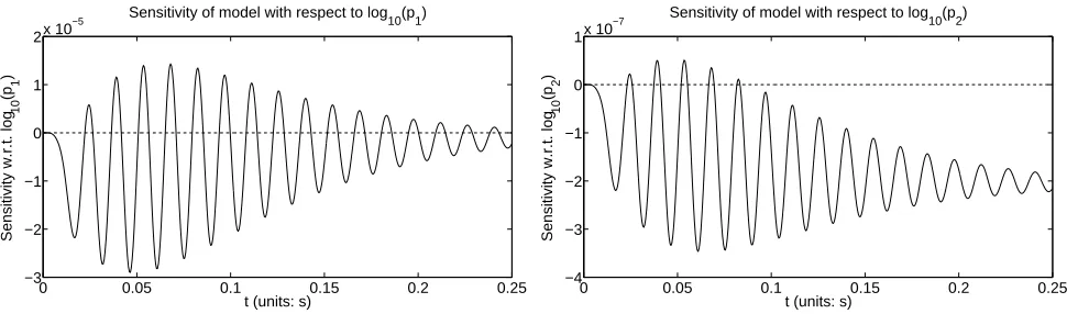
Figure 7 demonstrates the sensitivities of model output with respect to material weights log₁₀(p1)

and log₁₀(p2). From this figure we see that the model is less sensitive to the second weighting than to

0 0.05 0.1 0.15 0.2 0.25 −3

−2 −1 0 1 2x 10

−5

t (units: s)

10

(p 1

)

10(p1)

0 0.05 0.1 0.15 0.2 0.25 −4

−3 −2 −1 0 1x 10

−7

t (units: s)

10

(p2

)

10(p2)

Figure 7: (left pane) Sensitivity of model output with respect to log10(p1); and (right pane)

Sen-sitivity of model output with respect to log₁₀(p2). Again, both sensitivities around the baseline

parameters (6) and forcing function with parametersa= 6×10−3_, _b_{= 20}_×₁₀−3_{, and}_A_{= 6}_×₁₀3_.

the first one. In future work when we turn to consider estimating the weights (instead of specifying them as we do in this work), we can predict that accurately estimating the second material weighting will be much more difficult than estimating the first one.

Armed with our knowledge of sensitivities of model output with respect to the material param-eters around the true parameter values (6), and our knowledge of effects on the model solution of changing the parameters, we can describe the generation of our simulated data and discuss solution of the inverse problem itself.

2.3 Statistical model and inverse problem

We will work with simulated data for various noise levels generated at position x = L, namely data uj corresponding with model solution u(L, tj) at measurement time points tj = 0.001j,

j = 0,1, . . . ,250. Thus, there are a total of n = 251 data points. For the current proof of con-cept discussion, we will assume the measurement errors Ej are independent, identically, normally distributed with mean zero (E(Ej) = 0) and constant variance var(Ej) =σ02. We thus are

(12)

assumptions correspond with the error process

Uj =u(L, tj; 10θ) +Ej, j = 0,1, . . . , n−1, (9)

where u(L, tj; 10θ) is the solution to (1), (3) and (4) along with (5) at x = L with a given set of material parameters θ. For realizations ǫj of Ej, corresponding realizations of Uj are given by

uj =u(L, tj; 10θ) +ǫj, j = 0,1, . . . , n−1. (10)

Under the error assumption framework (9), we now define the estimator ˆΘ to be

ˆ

Θ = arg min

θ∈Q

n−1

X

j=0

Uj−u(L, tj; 10θ)

2

, (11)

where Q ⊂ Rκ is some viable admissible parameter set, assumed compact in Rκ with κ being the number of parameters requiring estimation. Note that under different error assumptions, one would need to modify the cost function in (11) (a topic discussed in [BaTr]) for an appropriate asymptotic parameter distribution theory to be valid. Since ˆΘ is a random variable (inherited from the fact that the errorsEj are random variables), we can define its corresponding realizations by (using data realizations (10), either simulated or from an experiment)

ˆ

θ= arg min

θ∈Q

n−1

X

j=0

uj −u(L, tj; 10θ)

2

. (12)

Estimating material parameters ˆθ from given sets of data with different noise levels, as well as quantifying uncertainty in our estimate, will be the key focus of our work in this section. For these purposes, we will assume that the material density and the weights pi for each relaxation time are known and given in either (7) or (8) (depending on the number of relaxation times to be estimated). Though in reality one would certainly need to estimate the weights pi, we take the liberty here of assuming them to be known so we can focus on the general methodology and in particular the identifiability of the relaxation times. We also use the values for E0, E1, τ1, and τ2 in (6) in their

log scaled form as the baseline values θ0 used in simulating data. That is,

θ0 = (5.3424,1.6021,−1.3010,1)T = (log10(2.2×105),log1040,log10.05,log1010)T

(13)

2.3.1 Data generation

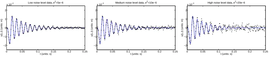
As noted previously, we will simulate data using two relaxation times (and a question of interest later will be how many of those relaxation times we can recover). With the values of parameters given in (6), noiseless data has maximum amplitude on the order of 10−4 _{(shown in Figure 3). This}

level informs the magnitude we choose for the additive noise. We represent a “low” noise level with σ₀2 = 5×10−6_{, a “medium” noise level by} _σ2

0 = 10×10

−6_{, and a “high” noise level by taking}

σ2

0 = 20×10

−6_{. In Figure 8, we show plots corresponding to the three levels of noisy simulated}

0 0.05 0.1 0.15 0.2 0.25

−2 −1 0 1 2

x 10−4

t (units: s)

u(L,t) (units: m)

Low noise level data, σ2

=5e−6

0 0.05 0.1 0.15 0.2 0.25

−2 −1 0 1 2

x 10−4

t (units: s)

u(L,t) (units: m)

Medium noise level data, σ2

=10e−6

0 0.05 0.1 0.15 0.2 0.25

−2 −1 0 1 2

x 10−4

t (units: s)

u(L,t) (units: m)

High noise level data, σ2

=20e−6

Figure 8: Simulated noisy data around the true parameter values. (left pane) Low noise level,

σ₀2 = 5× 10−6_{. (middle pane) Medium noise,} _σ2

0 = 10 ×10

−6_{. (right pane) High noise level,}

σ₀2 = 20×10−6_.

data against the system dynamics corresponding to the true parameters. Noise is assumed absolute for our initial investigations (though we may ultimately need to explore relative noise once an error model is developed for our experimental data), and is added according to the error model (10). Low noise results in data mostly along the trajectory of the true model. Medium noise begins to obfuscate the later-time oscillations which have lost much of their earlier energy. High noise significantly affects the level of peaks and troughs fromt= 0.05 forward. We thus obtain a series of increasingly difficult problems in obtaining material parameter estimates, though entirely expected since higher noise tends to significantly affect data features and presents a more difficult parameter estimation problem.

2.3.2 Inverse problem, different optimization routines

In this section, we discuss different options for the optimization routine used to solve (12), and begin to gain a sense of the robustness of parameter estimation with respect to the optimization routine. Note that we expect to have some difficulty in relaxation time estimation, based on our earlier discussion on the model response to changes in relaxation times as well as model sensitivities. We do expect to obtain more accurate estimates for E1, and very good estimates for E0. To begin

this discussion, we will examine parameter estimates for a model which incorporates two relaxation times.

The optimization routines we compare are all built-in Matlab routines. We use fmincon with

(14)

option. Note that the Levenburg-Marquardt algorithm does not allow bound constraints; we tried the routine out of curiosity, to see if it would produce unrealistic estimates of any parameters (it does at high noise levels).

Results from optimizing for θ are shown in Tables 1-3. All optimization runs used the initial guess

θinit= (log10(1.8×105),log10(60),log10(0.5),log10(20))T = (5.2553,1.7782,−0.3010,1.3010)T.

All these tables include the parameter estimates for ˆθ, computation time for that particular opti-mization run, and the residual sum of squares (RSS) defined as

RSS =

n−1

X

j=0

h

uj −u(L, tj; 10

ˆ

θ₎i2_.

Overall, the routines do a good job (Tables 1-3) of estimating E0, as we expected. Thelsqnonlin

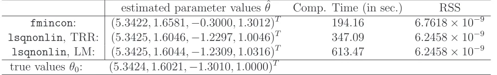
Table 1: Estimation of material parameters in the case of low noise σ02 = 5×10

−6_{: Comparison}

between optimization routines (TRR=trust-region-reflective, LM=Levenburg-Marquardt). estimated parameter values ˆθ Comp. Time (in sec.) RSS

fmincon: (5.3422,1.6581,−0.3000,1.3012)T 194.16 6.7618×10−9

lsqnonlin, TRR: (5.3425,1.6046,−1.2297,1.0046)T 347.09 6.2458×10−9

lsqnonlin, LM: (5.3425,1.6044,−1.2309,1.0316)T 613.47 6.2458×10−9

true values θ0: (5.3424,1.6021,−1.3010,1.0000)T

Table 2: Estimation of material parameters with medium noiseσ₀2 = 10×10−6

: Comparison between optimization routines (TRR=trust-region-reflective, LM=Levenburg-Marquardt).

estimated parameter values ˆθ Comp. Time (in sec.) RSS

fmincon: (5.3430,1.6583,−0.2998,1.3012)T 203.75 2.4435×10−8

lsqnonlin, TRR: (5.3433,1.5889,−1.3269,2.0000)T 241.51 2.3647×10−8

lsqnonlin, LM: (5.3433,1.5893,−1.3252,5.9303)T 608.27 2.3646×10−8

true values θ0: (5.3424,1.6021,−1.3010,1.0000)T

Table 3: Estimation of material parameters in the case of high noise σ₀2 = 20×10−6

: Comparison between optimization routines (TRR=trust-region-reflective, LM=Levenburg-Marquardt).

estimated parameter values ˆθ Comp.Time(s.) RSS

fmincon: (5.3433,1.6380,−0.2995,1.3012)T 238.58 1.03291×10−7 lsqnonlin, TRR: (5.3433,1.6361,−1.990,0.2496)T 606.36 1.03257×10−7

lsqnonlin, LM: (5.3433,1.6351,−0.02324,3.6112×10−4₎T _1110.83 ₁_.₀₃₂₄₈_×₁₀−7

(15)

routines tend to better estimate E1. As for relaxation times, we begin to see a major flaw in the

fmincon routine. It does not seem particularly sensitive to the relaxation times, and the resulting estimates of the relaxation times stay near the initial guess. Thefmincon routine produced similar

non-responsive results for different initial guesses. Thelsqnonlin routines estimate the relaxation times well in the presence of low noise (Table 1). At medium noise (Table 2), the routines estimateτ1

well but notτ2. At high noise (Table 3), relaxation time estimation is poor. This will be quantified

further in the following sections on error analysis.

Even though there might be some spurious computation times on desktop machines (due to other background programs), we still include them here to demonstrate typical optimization rou-tine performance. Consistently, fmincon was the fastest routine. This is in part due to the fact that this routine alone of the three supports parallel computation, so on our multi-core desktop machines we were able to see a speed-up. However, the computation times for the trust-region-reflective lsqnonlin algorithm are reasonable. Using Levenburg-Marquardt consistently is the slowest method, and the results are not better than those using trust-region-reflective lsqnonlin

algorithm.

As a result, we recommend using the trust-region-reflectivelsqnonlinalgorithm when trying to estimate relaxation times. If the model does not contain relaxation times (i.e., only estimating E0

andE1), the speedup afforded by usingfmincon may make that algorithm the one of choice. Figure

9 illustrates model fits to the data at different noise levels, where the model solution is calculated with the values of model parameters obtained throughlsqnonlinTRR routine. We see in all cases that the model solution provides reasonable fits to the data.

2.3.3 Asymptotic error analysis

Most asymptotic error theory [BaTr, BaHoRo] is described in the context of an ODE model example ˙

z(t) = g(z(t;θ);θ). However, we can use the PDE sensitivities of the model state with respect to

each parameter in θ, namely ∂u(x, t; 10

θ₎

∂θi

, in a similar manner to the ODE sensitivities in the

asymptotic theory. The steps of the asymptotic theory error analysis are as follows (the theory for the following steps is described in [BaTr, BaHoRo]).

1. Determine ˆθ by computing (12).

2. Compute the sensitivity equations to obtain ∂u(x, t; 10

ˆ

θ₎

∂θi

(as discussed in Section 2.2) for

i = 1, . . . , κ where κ is the number of parameters being estimated. Since data is only taken at position x=L, only the values at x=L will be used to form the sensitivity matrix χ(ˆθ). This matrix then has entries

χj,i(ˆθ) =

∂u(L, tj; 10

ˆ

θ₎

∂θi

, j = 0,1, . . . , n−1, and i= 1, . . . , κ.

Note that χ(ˆθ) is then an n ×κ matrix. We can also obtain an estimate for the constant variance σ₀2 as

ˆ

σ2 = 1

n−κ

n−1

X

j=0

uj −u(L, tj; 10

ˆ

(16)

0 0.05 0.1 0.15 0.2 0.25 −2

−1 0 1 2

x 10−4

t (units: s)

u(L,t) (units: m)

Solution at lsqnonlin parameter estimate, low noise data

0 0.05 0.1 0.15 0.2 0.25 −2

−1 0 1 2

x 10−4

t (units: s)

u(L,t) (units: m)

Solution at lsqnonlin parameter estimate, med noise data

0 0.05 0.1 0.15 0.2 0.25 −2

−1 0 1 2

x 10−4

t (units: s)

u(L,t) (units: m)

Solution at lsqnonlin parameter estimate, high noise data

Figure 9: Data and two-relaxation-time model solutions at parameter estimates obtained using

lsqnonlin, trust-region-reflective method, at different noise levels (see Tables 1-3). (upper pane)

(17)

3. Asymptotic theory yields that the estimator ˆΘ is asymptotically (as sample size n → ∞) normal with mean approximated by ˆθ and the covariance matrix approximated by

Cov( ˆΘ)≈Σ = ˆˆ σ2[χT(ˆθ)χ(ˆθ)]−1 .

4. The standard errors for each element in the parameter estimator ˆΘ can be approximated by

SE( ˆΘi) =

q

ˆ

Σii, i= 1,2, . . . , κ,

where ˆΘi is the ith element of ˆΘ, and ˆΣii is the (i, i)th entry of the matrix ˆΣ. Hence, the endpoints of the confidence intervals for ˆΘi are given by

ˆ

θi±t1−α/2SE( ˆΘi)

for i = 1,2, . . . , κ. Here t1−α/2 is a distribution value that is determined from a statistical

table for Student’s t-distribution based on the level of significance α (i.e., α =.05 for a 95% confidence interval).

We will present results below in Tables 4-9 on the low, medium, and high noise data sets using zero, one, and two relaxation times, and using the routines fmincon and lsqnonlin

(trust-region-reflective only, as we cannot enforce the bound constraints with the Levenburg-Marquardt algorithm). We see throughout the tables that the problem of estimating the second relaxation time is fraught with difficulty (the standard error is significantly higher than its estimated value), even though we know the simulated data came from a model incorporating two relaxation times. This was foreshadowed in our earlier examination of the sensitivities with respect to the second relaxation time, as well as the results for relaxation times seen when using different optimization routines. In addition, when estimating two relaxation times using lsqnonlin on high noise data (shown in Table 9(c)) we see that the estimates for τ1 and τ2 are not close to the true parameter

values; also, the standard error forτ1 is much larger than in any other case. Thus, instead of merely

having difficulty estimating a second relaxation time, in this estimation we now additionally have a less confidence on the estimate of τ1.

From Tables 4-6 we see that standard errors for E0 and E1 for the model with no relaxation

times are comparable with those for the model with one relaxation time when using fmincon, but the standard error for τ1 is fairly large (around 7, as compared with the estimated parameter value

log₁₀( ˆτ1) ≈ −0.3). When using lsqnonlin (see Tables 7-9), the standard errors for E0 and E1

increase significantly at all noise levels when moving from the no relaxation time model to the one relaxation time model, but the standard error for τ1 is closer to 2 rather than the 7 for fmincon.

This may not seem significant, but if we recall that these are log-scaled parameter values, then the difference between standard errors of 2 and 7 is significant and an indication that lsqnonlin may be the better procedure.

We also found that at all noise levels the difference for the residual sum of squares is small among the no-relaxation-time, one-relaxation-time, and two-relaxation-time models using either fmincon

(18)

Table 4: Low noise,fmincon: Parameter estimates, asymptotic standard errors (SE) and confidence

intervals

(a) No relaxation times

True Value Estimate SE 95% Confidence Interval

log₁₀(E0) 5.3424 5.3422 0.01373 (5.3223, 5.3622)

log₁₀(E1) 1.6021 1.6651 0.1052 (1.4579, 1.8723)

(b) One relaxation time

log₁₀(E0) 5.3424 5.3422 0.01012 (5.3223, 5.3622)

log10(E1) 1.6021 1.584 0.1436 (1.3757, 1.9412)

log₁₀(τ1) -1.3010 -0.3002 6.9746 (-1.4037, 1.3437)

(c) Two relaxation times

log₁₀(E0) 5.3424 5.3422 0.1014 (5.3223, 5.3622)

log₁₀(E1) 1.6021 1.6581 0.1463 (1.3700, 1.9463)

log10(τ1) -1.3010 -0.3000 8.2619 (-16.5727, 15.9828)

log₁₀(τ2) 1 1.3012 51.0143 (-99.1775, 101.7798)

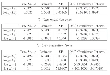
Table 5: Medium noise, fmincon: Parameter estimates, asymptotic standard errors (SE) and con-fidence intervals

log10(E0) 5.3424 5.3264 0.01409 (5.3087, 5.3542)

log10(E1) 1.6021 1.7641 0.01165 (1.5346, 1.9936)

log10(E0) 5.3424 5.3430 0.01032 (5.3226, 5.3633)

log₁₀(E1) 1.6021 1.6586 0.1462 (1.3706, 1.9467)

log₁₀(τ1) -1.3010 -0.3001 7.1076 (-1.4299, 1.3699)

log₁₀(E0) 5.3424 5.3430 0.01034 (5.3226, 5.3633)

log10(E1) 1.6021 1.6583 0.1490 (1.3648, 1.9519)

log₁₀(τ1) -1.3010 -0.2998 8.4206 (-16.8851, 16.2855)

(19)

Table 6: High noise,fmincon: Parameter estimates, asymptotic standard errors (SE) and confidence

intervals

log₁₀(E0) 5.3424 5.3433 0.01046 (5.3227, 5.3639)

log₁₀(E1) 1.6021 1.6452 0.1136 (1.4214, 1.8691)

log₁₀(E0) 5.3424 5.3433 0.01045 (5.3227, 5.3639)

log10(E1) 1.6021 1.6382 0.1600 (1.3232, 1.9534)

log₁₀(τ1) -1.3010 -0.2995 7.7134 (-15.4916, 14.8927)

log₁₀(E0) 5.3424 5.3433 0.01047 (5.3227, 5.3639)

log₁₀(E1) 1.6021 1.6380 0.1633 (1.3164, 1.9596)

log10(τ1) -1.3010 -0.2995 9.1380 (-18.2979, 17.6989)

log₁₀(τ2) 1 1.3012 56.4222 (-109.8289, 112.4314)

Table 7: Low noise, TRR lsqnonlin: Parameter estimates, asymptotic standard errors (SE) and confidence intervals

log10(E0) 5.3424 5.3422 4.9498×10−4 (5.3413, 5.3432)

log10(E1) 1.6021 1.6651 0.005434 (1.6544, 1.6758)

log10(E0) 5.3424 5.3425 0.01011 (5.3226, 5.3624)

log₁₀(E1) 1.6021 1.6050 0.3167 (0.9811, 2.2288)

log₁₀(τ1) -1.3010 -1.2317 2.2200 (-5.6041, 3.1407)

log₁₀(E0) 5.3424 5.3425 0.0101 (5.3225, 5.3624)

log10(E1) 1.6021 1.6046 0.3202 (0.9738, 2.2353)

log₁₀(τ1) -1.3010 -1.2297 2.2369 (-5.635, 3.1761)

(20)

Table 8: Medium noise, TRR lsqnonlin: Parameter estimates, asymptotic standard errors (SE)

and confidence intervals

log₁₀(E0) 5.3424 5.3429 9.2836×10−4 (5.3411, 5.3448)

log₁₀(E1) 1.6021 1.6653 0.0102 (1.6452, 1.6854)

log₁₀(E0) 5.3424 5.3433 0.01042 (5.3228, 5.3638)

log10(E1) 1.6021 1.6050 0.3167 (0.9811, 2.2288)

log₁₀(τ1) -1.3010 -1.2317 2.2200 (-5.6041, 3.1407)

log₁₀(E0) 5.3424 5.3433 0.01045 (5.3227, 5.3639)

log₁₀(E1) 1.6021 1.5889 0.3717 (0.8567, 2.3211)

log10(τ1) -1.3010 -1.3269 2.0383 (-5.3415, 2.6878)

log₁₀(τ2) 1 2.0000 156.5630 (-306.369, 310.369)

Table 9: High noise, TRR lsqnonlin: Parameter estimates, asymptotic standard errors (SE) and confidence intervals

log10(E0) 5.3424 5.3433 1.7767×10−3 (5.3398, 5.3468)

log10(E1) 1.6021 1.6452 0.0204 (1.6050, 1.6855)

log10(E0) 5.3424 5.3433 0.01046 (5.3227, 5.3639)

log₁₀(E1) 1.6021 1.6397 0.1526 (1.3391, 1.9403)

log₁₀(τ1) -1.3010 -1.3253 2.0328 (-5.3291, 2.6785)

log₁₀(E0) 5.3424 5.3433 0.01046 (5.3227, 5.3639)

log10(E1) 1.6021 1.6361 0.1591 (1.3227, 1.9496)

log₁₀(τ1) -1.3010 -0.1990 15.8821 (-31.4806, 31.0827)

(21)

Model selection criteria There are numerous model selection criteria in the literature that can be used to select a best approximating model from a prior set of candidate models. These criteria are based either on hypothesis testing or mean squared error or Bayes factors or information theory, and they all are based to some extent on the principle of parsimony (see [BuAn]). It should be noted that some of these criteria can only be used for nested models (e.g., two models are said to be nested if one model is a special case of the other), but others can be used for both nested models and non-nested models. Here we employ one of the most widely used model selection criteria – the Akaike information criterion (AIC). The AIC was developed by Akaike (in 1973) who formulated a relationship between the Kullback-Leibler information (used to measure the information lost when a model is used to approximate the full reality) and the maximum value of the log likelihood function of the approximating model. As might be expected we find that the AIC value depends on the data set used. Thus, when we try to select a best model from a set of candidate models, we must use the same data set to calculate AIC values for each of the models. One of the advantages of the AIC is that it can be used to compare non-nested models (which is our case here). For the least squares case, it can be found (e.g., see [BuAn, Section 2.2]) that if the observation errors are i.i.d normally distributed, then the AIC is given by

AIC =nlog

RSS

n

+ 2(κ+ 1). (13)

Here κ + 1 is the total number of estimated parameters including θ and the observation error variance. Given a prior set of candidate models, we can calculate the AIC value for each model, and the best approximating model is the one with minimum AIC value. It should be noted that the AIC may perform poorly if the sample size n is small relative to the total number of estimated parameters (it is suggested in [BuAn] that the sample size n should be at least 40 times the total number of estimated parameters (κ+ 1); note this is true for our investigations).

In practice, the absolute size of the AIC value may have limited use in supporting the chosen best approximating model, and one may often employ other related values such as Akaike differences and Akaike weights to further compare models. The Akaike difference is defined by

∆i =AICi−AICmin, i= 1,2, . . . R, (14)

whereAICi is the AIC value of theith model in the set, AICmindenotes theAIC value for the best

model in the set, and R is the total number of models in the set. The larger ∆i, the less plausible it is that theith model is a good approximating model for given the data set. The Akaike weights are defined by

wi=

exp(−1 2∆i)

PR

r=1exp(−12∆r)

, i= 1,2, . . . R. (15)

These Akaike weights wi can then be interpreted as the probability that ith model is the best approximating model (see [BuAn]).

(22)

Table 10: fmincon: Residual sum of squares (RSS), AIC values, AIC differences (∆) and AIC

weights for zero-relaxation-time model (model 0), one-relaxation-time model (model 1) and two-times-relaxation model (model 2) obtained at low, medium and high noise levels.

noise level model RSS AIC ∆ AIC weights

low noise

0 7.0368×10−9 _-6.0927_×₁₀3 _7.5867 _1.5257_×₁₀−2

1 6.7731×10−9

-6.1003×103 0 6.7748×10−1

2 6.7618×10−9 _-6.0987_×₁₀3 _1.5814 _3.0726_×₁₀−1

medium noise

0 3.6421×10−8

-5.6800×103 98.1093 3.5908×10−22

1 2.4442×10−8 _-5.7782_×₁₀3 ₀ _7.2334_×₁₀−1

2 2.4435×10−8 _-5.7762_×₁₀3 _1.9222 _2.7666_×₁₀−1

high noise

0 1.0337×10−7 _-5.4182_×₁₀3 ₀ _6.4532_×₁₀−1

1 1.0330×10−7 _-5.4164_×₁₀3 _1.8267 _2.5889_×₁₀−1

2 1.0329×10−7

-5.4144×103 3.8151 9.5794×10−2

Table 11: lsqnonlin: Residual sum of squares (RSS), AIC values, AIC differences (∆) and AIC weights for zero-relaxation-time model (model 0), one-relaxation-time model (model 1) and two-times-relaxation model (model 2) obtained at low, medium and high noise levels.

noise level model RSS AIC ∆ AIC weights

low noise

0 7.0368×10−9 _-6.0927_×₁₀3 _{27.8791 6.4125}_×₁₀−7

1 6.2470×10−9 _-6.1206_×₁₀3 ₀ _7.2595_×₁₀−1

2 6.2458×10−9

-6.1186×103 1.9483 2.7405×10−1

medium noise

0 2.4674×10−8 _-5.7778_×₁₀3 _8.6863 _9.4255_×₁₀−3

1 2.3646×10−8 _-5.7865_×₁₀3 ₀ _7.2527_×₁₀−1

2 2.3647×10−8 _-5.7845_×₁₀3 _2.0113 _2.6531_×₁₀−1

high noise

0 1.0337×10−7

-5.4182×103 0 6.4303×10−1

1 1.0330×10−7 _-5.4164_×₁₀3 _1.8299 _2.5756_×₁₀−1

2 1.0326×10−7 _-5.4145_×₁₀3 _3.7340 _9.9406_×₁₀−2

one-relaxation-time model is the best with the probability to be chosen as the best model being more than 0.6 (see the Akaike weights in the last column of these two tables), and the no-relaxation time model has almost no chance of being selected as the best. For the high noise data set, the no-relaxation-time model is the best, with the probability of being chosen as the best being more than 0.6, while the two-relaxation-time model has little chance of being selected as the best model.

(23)

2.3.4 Bootstrapping error analysis

For ease of presentation, we reiterate here the algorithm described in [BaHoRo], in the context of the current viscoelastic model under study.

1. Determine ˆθ0 by computing (12).

2. Define the standardized residuals (recalln is the number of data points, andκ is the number of parameters under consideration) to be

¯

rj =

r

n n−κ

uj−u(L, tj; 10

ˆ

θ0

)

for j = 0,1, . . . , n−1. Setm = 0.

3. Create a sample of size n by randomly sampling, with replacement, from the standardized residuals ¯rj to form a bootstrap sample {rm0 , . . . rnm−1}.

4. Create bootstrap sample points um_j =u(L, tj; 10

ˆ

θ0

) +r_jm for j = 0,1, . . . , n−1.

5. Solve the OLS minimization problem (12) with the bootstrap-generated data {um_j } to obtain a new estimate ˆθm+1 which we store.

6. Increase the index m by 1 and repeat steps 3-5. This iterative process should be carried out forM times whereM is large (we used M = 1000, as suggested in [BaHoRo]). This will give

M estimates {θˆm}M_m₌₁.

Upon completing allM simulation runs, the following will give the mean, covariance, and standard errors for the bootstrap estimator ˆΘboot:

ˆ

θboot = 1

M

X

m=1

ˆ

θm,

ˆ

Σboot = 1

M −1 M

X

m=1

(ˆθm−θˆboot)(ˆθm−θˆboot)T,

(SEboot)i =

r

ˆ Σboot

ii, i= 1,2, . . . , κ,

(16)

whereΣˆboot

iiis the (i, i)th entry of covariance matrix ˆΣboot. Hence, the endpoints of the confidence intervals for ( ˆΘboot)i (the ith element of ˆΘboot) are given by

(ˆθboot)i±t1−α/2(SEboot)i

for i= 1,2, . . . , κ.

(24)

the model multiple times). Due to long computational times (e.g., one week for bootstrapping versus minutes for the asymptotic theory), we report here results only for a case using fminconto estimate

E0 and E1 in a zero-relaxation-time model and a case using lsqnonlin, the trust-region-reflective

method, to estimate E0, E1, and τ1 in a one-relaxation-time model. It is worth noting that even

though the bootstrapping algorithm can be implemented in parallel, this requires a considerable amount of computing resources (unavailable to most investigators) to achieve computational times comparable to that attained in using the asymptotic theory. For our purposes, the bootstrap results we provide are sufficient to indicate that the less conservative asymptotic error analysis yields a reasonable uncertainty measure in the inverse problem we investigate.

For the model with no relaxation times, we see from Table 12 that the confidence intervals for

E0 and E1 at all noise levels are more conservative (as expected-see [BaHoRo]) than those obtained

using the asymptotic theory (shown in Tables 4(a), 5(a) and 6(a)), especially for the cases of medium and high noise level. However, this table still indicates that reasonable parameter estimates are obtained.

Table 12: Bootstrapping results, no relaxation times, using fmincon: Parameter estimates, boot-strap standard errors (SE) and confidence intervals

(a) Low noise level

True Value θˆboot SE 95% Confidence Interval log10(E0) 5.3424 5.3422 0.01557 (5.3115, 5.3729)

log₁₀(E1) 1.6021 1.6649 0.1716 (1.3270, 2.0029)

(b) Medium noise level

log10(E1) 1.6021 1.6653 0.3155 (1.0438, 2.2867)

(c) High noise level

log₁₀(E1) 1.6021 1.6451 0.6603 (0.3446, 2.9456)

In Figure 10, we depict the bootstrap estimates obtained for E0 and E1 for this no relaxation

time model. Note that each empirical distribution (a representation for the estimator distribution) tends to have the shape of a normal distribution, which we would expect if bootstrapping is working properly.

We also present bootstrapping results for a model incorporating one relaxation time. The inverse problem solved during the bootstrap procedure was computing using lsqnonlin, the

(25)

5.34050 5.341 5.3415 5.342 5.3425 5.343 5.3435 5.344 20 40 60 80 100 Values Count

Boostrap values for (log−scaled) E₀, model with no relaxation times

1.6450 1.65 1.655 1.66 1.665 1.67 1.675 1.68 1.685 1.69

20 40 60 80 100 Values Count

Boostrap values for (log−scaled) E₁, model with no relaxation times

5.340 5.341 5.342 5.343 5.344 5.345 5.346 5.347

20 40 60 80 100 120 Values Count

Boostrap values for (log−scaled) E

0, model with no relaxation times

1.620 1.64 1.66 1.68 1.7 1.72 1.74

20 40 60 80 100 120 Values Count

1, model with no relaxation times

5.336 5.3380 5.34 5.342 5.344 5.346 5.348 5.35 5.352 5.354

20 40 60 80 100 120 Values Count

Boostrap values for (log−scaled) E₀, model with no relaxation times

1.560 1.58 1.6 1.62 1.64 1.66 1.68 1.7 1.72

20 40 60 80 100 120 Values Count

Boostrap values for (log−scaled) E₁, model with no relaxation times

Figure 10: Histograms of bootstrap estimates ˆθm for a model with no relaxation times in the case of low noise data set (upper row), medium noise data set (middle row) and high noise data set (bottom row). (left column) Estimates for log₁₀(E0); (right column) Estimates for log10(E1).

magnitude than the relaxation time value itself. This is even more prominent at higher noise levels – the results in the table indicate that on medium and high noise data sets, the estimation of τ1 is

not very robust. Note also that the estimation of E1 begins to suffer as well, resulting in a higher

standard error than its own value on the high noise data set. This is a further indication that we may have problems in the future estimating even the single relaxation time.

We depict histograms of the estimates in Figure 11. We see on a low noise data set that each parameter estimator appears to be mostly normally distributed. This begins to break down for the case of middle noise level data set (shown in the middle row of Figure 11), where we begin to see some outliers at the log₁₀(ˆτ1) = 2 level (which means the estimates were converging to our upper

bound on that parameter) and also some more pronounced skewness in the count levels. Finally, on the high noise level (shown in bottom row of Figure 11) we have the distribution for the E1

(26)

Table 13: Bootstrapping results, one relaxation time, using lsqnonlin: Parameter estimates, boot-strap standard errors (SE) and confidence intervals

(a) Low noise level

True Value θboot SE 95% Confidence Interval

log10(E0) 5.3424 5.3425 0.01547 (5.3120, 5.3730)

log₁₀(E1) 1.6021 1.6025 0.5937 (0.4332, 2.7719)

log10(τ1) -1.3010 -1.2294 3.8697 (-8.8510, 6.3923)

(b) Medium noise level

log₁₀(E0) 5.3424 5.3434 0.03136 (5.2816, 5.4052)

log10(E1) 1.6021 1.5852 1.4590 (-1.2884, 4.4589)

log10(τ1) -1.3010 -1.2079 16.9971 (-34.6849, 32.2692)

(c) High noise level

log10(E0) 5.3424 5.3434 0.061762 (5.2218, 5.4651)

log₁₀(E1) 1.6021 1.6029 2.4545 (-3.2314, 6.4372)

(27)

5.34050 5.341 5.3415 5.342 5.3425 5.343 5.3435 5.344 5.3445 20 40 60 80 100 120 Values Count

Boostrap values for (log−scaled) E₀, model with one relaxation time

1.520 1.54 1.56 1.58 1.6 1.62 1.64 1.66 1.68

20 40 60 80 100 120 Values Count

Boostrap values for (log−scaled) E₁, model with one relaxation time

−1.60 −1.4 −1.2 −1 −0.8 −0.6

20 40 60 80 100 120 Values Count

Boostrap values for (log−scaled) τ1, model with one relaxation time

5.3380 5.34 5.342 5.344 5.346 5.348 5.35

20 40 60 80 100 120 Values Count

0, model with one relaxation time

1.40 1.45 1.5 1.55 1.6 1.65 1.7 1.75 1.8 1.85

20 40 60 80 100 120 Values Count

1, model with one relaxation time

−20 −1.5 −1 −0.5 0 0.5 1 1.5 2 2.5

50 100 150 200 250 300 Values Count

5.336 5.3380 5.34 5.342 5.344 5.346 5.348 5.35 5.352 5.354

20 40 60 80 100 120 140 Values Count

Boostrap values for (log−scaled) E₀, model with one relaxation time

0.90 1 1.1 1.2 1.3 1.4 1.5 1.6 1.7 1.8

50 100 150 200 250 300 350 Values Count

Boostrap values for (log−scaled) E₁, model with one relaxation time

−30 −2 −1 0 1 2 3

50 100 150 200 250 Values Count

Figure 11: Histograms of bootstrap estimates ˆθm for a model with one relaxation time in the case of low noise data set (upper row), medium noise data set (middle row) and high noise data set (bottom row). (left column) Estimates for log₁₀(E0); (middle column) Estimates for log10(τ1); (right column)

(28)

3 Model comparison and hypothesis testing on amplitude

In this section, we develop a methodology for determining whether or not data came from a low-amplitude input traction. This corresponds with determining if the data came from a vessel expe-riencing a normal heartbeat or not. We will ultimately run the inverse problem without amplitude restrictions and use a scoring function to compare results with the score of the model solved at a low amplitude. A model comparison test will be implemented to determine if there is a statistical significance in the differences between the model solved with the unrestricted estimate and the model solved using the restricted amplitude value.

3.1 Setup

We first examine the sensitivity of the model with respect to the Van Bladel input amplitude parameter A, to be sure that an estimation procedure is reasonable (if the model were insensitive toA then the results from the optimization routine would be suspect). The form of the sensitivity equation is nearly identical to that of the actual model, just with a lower amplitude. This is seen in Figure 12, which has a form similar to that of the model solution (Figure 3). In both the low and high amplitude cases, the sensitivity with respect to amplitude is most marked during early times and less so at later times; this makes perfect sense, as the amplitude is greater early on before being damped out. In the problem below, we will take data throughout the full time frame t ∈ [0,0.25] so with our sensitivity results we can be assured that the early data will drive estimation of the amplitude parameter.

0 0.05 0.1 0.15 0.2 0.25 −6

−4 −2 0 2 4x 10

−4

t (units: s)

10

(A)

High amplitude; sensitivity of model with respect to log

10(A)

0 0.05 0.1 0.15 0.2 0.25 −6

−4 −2 0 2 4x 10

−5

t (units: s)

10

(A)

Low amplitude; sensitivity of model with respect to log

10(A)

Figure 12: Sensitivity of model with respect to Van Bladel input parameter A around the baseline parameters (6). (left pane) High forcing function amplitude A= 6×103. (right pane) Low forcing function amplitude A= 6×102.

3.2 Data generation

(29)

data set will be generated with variance σ2 = 5×10−7_{, medium noise with} _σ2 _{= 10}_×₁₀−7_{, and}

high noise with σ2 = 20×10−7_{. The low amplitude input data set then is supposed to represent a}

normal heartbeat and the high amplitude data set then is meant to represent the input shear for a heartbeat in the presence of a stenosis in the vessel. Note that we are not yet exactly certain regarding the difference between these effects in an actual patient, so the data sets here are truly for a proof-of-concept investigation. The low amplitude data sets are depicted in Figure 13.

0 0.05 0.1 0.15 0.2 0.25

−2 −1.5 −1 −0.5 0 0.5 1 1.5

x 10−5

t (units: s)

u(L,t) (units: m)

Low amplitude; low noise level data, σ2_=5e−7

0 0.05 0.1 0.15 0.2 0.25

−2 −1.5 −1 −0.5 0 0.5 1 1.5

x 10−5

t (units: s)

u(L,t) (units: m)

Low amplitude; medium noise level data, σ2_=10e−7

0 0.05 0.1 0.15 0.2 0.25

−2 −1.5 −1 −0.5 0 0.5 1 1.5

x 10−5

t (units: s)

u(L,t) (units: m)

Low amplitude; high noise level data, σ2_=20e−7

Figure 13: Simulated low amplitude noisy data around the true parameter values. (left pane) Low noise level, σ2

0 = 5×10

−7_{. (middle pane) Medium noise,} _σ2

0 = 10×10

−7_{. (right pane) High noise}

level, σ2₀ = 20×10−7_.

3.3 Hypothesis testing methodology

We can now begin to discuss the approach to model comparison and hypothesis testing that we will use by defining a model comparison test statistic. The work here follows the development in [BaTr]. Our performance criterion for hypothesis testing will be

J(U , θ~ ) =

n−1

X

j=0

[Uj−u(L, tj;θ)]2.

For the purposes of this paper, we postulate that a normal (non-stenosed) vessel corresponds with a low amplitude input parameterA≤6×102. Then, a stenosed vessel would have a high input amplitude parameter withA >6×102_{. The hypothesis test we use requires a set benchmark value}

for A, so we choose that benchmark to be A0 = 6×102. Then, we define the restricted parameter

set

AH ={A∈A|A=A0 = 6×102},

where A= [A0,∞) is the larger set of unrestricted admissible amplitudes.

Our null hypothesisH0 is that the amplitude is a low amplitude, represented byA∈AH ={A0}. The unrestricted amplitude model would then represent the amplitude parameter as A = A0 + ˜A

where ˜A ∈ [0,∞). This framework will allow us to develop a test statistic to determine the confidence level of accepting or rejecting H0 for a given data set. In other words, we will develop

a test to determine if the data is statistically better represented by the benchmark A0 than the

unrestricted amplitude.

(30)

needed to compute these values). We then run an optimization routine to determine an unrestricted input amplitude parameter estimate ˆθ, which we then use to computeJ(~u,θˆ). The value for ˆθcomes from solving the unrestricted optimization problem (12). As discussed in [BaTr, BaFi], the model comparison statistic is defined as

ˆ

V =nJ(U ,~ ΘˆH)−J(U ,~ Θ)ˆ J(U ,~ Θ)ˆ

with realization

ˆ

v =nJ(~u,θˆH)−J(~u,θˆ)

J(~u,θˆ) . (17)

If our null hypothesisH0 were true, the model comparison statistic ˆV converges in distribution to V

asn → ∞where V ∼χ2(r) is a chi-square distribution with r degrees of freedom (r is the number of constraints in AH). For our problem, r = 1. Given the significance level α, we can obtain a threshold value ν such that the probability that V will take on a value greater than ν is α. In other words, Prob(V > ν) =α. In our context, if the test statistic ˆv > ν we reject H0 as false with

confidence level (1−α)100%. Otherwise we do not reject H0 as false, at the specified confidence

level. In Table 14 we include sample values from theχ2_{(1) distribution for reference (table repeated}

from [BaTr]).

Table 14: Sample χ2(1) values.

α ν confidence

0.25 1.32 75%

0.1 2.71 90%

0.05 3.84 95%

0.01 6.63 99%

0.001 10.83 99.9%

We summarize in Table 15 the results of computing the OLS performance criterion for the low amplitude and high amplitude data each with the restricted/unrestricted parameters. Based on

Table 15: Model comparison test results using (17) on low, medium, and high noise data sets generated with both high and low input amplitude parameter A values.

J(~u,θˆ) J(~u,θˆH) vˆ

Low A, low noise 6.3846e-11 6.3887e-11 0.1609

Low A, medium noise 2.6872e-10 2.6896e-10 0.2258

Low A, high noise 9.8836e-10 9.9658e-10 2.0878

HighA, low noise 6.6812×10−9 _3.5229_×₁₀−7 _1.2984e+04

HighA, medium noise 3.1016×10−8

3.4730×10−7

2.5596e+03 High A, high noise 9.9737×10−8 _4.6015_×₁₀−7 _907.0283

(31)

lowA value that we do not reject H0 with high degrees of confidence. However, the case with high

noise is somewhat less certain, though we would still likely not reject H0 with a fairly high degree

of confidence. The results are more stark in the cases where the data was generated from a high amplitude. Given that the magnitude of ˆv is greater than 900 at all noise levels, we would reject

H0 as false on these data sets with confidence level more than 99.9%. Altogether, these results

suggest robustness in our methodology for determining whether the data came from a normal vessel experiencing a heartbeat (low input amplitude) or not.

4 Conclusion

In this work we have carried out proof-of-concept investigations for estimating material parame-ters and created a model comparison test as a basis for distinguishing between data that comes from a normal or from a stenosed blood vessel. We found that the model was less sensitive to a second viscoelastic relaxation time than to the other parameters, and this was manifested as a difficulty in recovering two relaxation times. On the other hand, models with zero or one relaxation time allowed for more confidence in the estimation procedure (i.e., smaller standard errors). We compared asymptotic error theory with bootstrapping error theory, and found (as expected) that bootstrapping gives more conservative confidence intervals but not so much so that the asymptotic theory cannot be profitably used for uncertainty quantification in models with large computational costs rendering bootstrapping less desirable. In terms of the model comparison on the input ampli-tude parameter A, we were able to develop a successful methodology for statistically determining whether or not data came from a low amplitude input force. This will form the basis of a model comparison test we can use on experimental data sets.

In future efforts, as already mentioned we will need to develop a procedure for estimating the material weightspi. This may involve iterating optimization routines to take advantage of features of

fmincon for estimating the weights, while using the routine lsqnonlin for the remaining material

parameters. We also plan to examine the possibility of relative error instead of absolute error, which will necessitate a generalized least squares (GLS) cost function in our inverse problems due to changes in the error process. This will be coupled with a study of a statistical model for the measurement processes being used in the experiments at QMUL. The changes needed are discussed in [BaTr]. If we require a GLS framework, we will need to derive a proper model comparison framework for GLS problems. The most important immediate efforts will be to apply the methods presented in this paper to the data from the QMUL experiments.

5 Acknowledgements

(32)

References

[BBETW] H.T. Banks, J.H. Barnes, A. Eberhardt, H. Tran, and S. Wynne, Modeling and compu-tation of propagating waves from coronary stenoses, Computation and Applied Mathematics,

21 (2002), 767–788.

[BaFi] H.T. Banks and B.G. Fitzpatrick, Inverse problems for distributed systems: statistical tests and ANOVA, LCDS/CCS Rep. 88-16, July, 1988, Brown University; Proc. International Sym-posium on Math. Approaches to Envir. and Ecol. Problems, Springer Lecture Notes in Biomath.,

81 (1989), 262–273.

[BaHoRo] H.T. Banks, K. Holm and D. Robbins, Standard error computations for uncertainty quan-tication in inverse problems: Asymptotic theory vs. Bootstrapping, CRSC-TR09-13, North Carolina State University, June 2009; Revised May 2010; Mathematical and Computer Mod-elling, 52 (2010), 1610–1625.

[BaHuKe] H.T. Banks, S. Hu, Z.R. Kenz, A brief review of elasticity and viscoelasticity for solids, Advances in Applied Mathematics and Mechanics,3 (2011), 1–51.

[BaLu] H.T. Banks and N. Luke, Modeling of propagating shear waves in biotissue employing an internal variable approach to dissipation, Communication in Computational Physics,3(2008), 603–640.

[BaMedPint] H.T. Banks, N. Medhin, and G. Pinter, Multiscale considerations in modeling of nonlinear elastomers,International Journal for Computational Methods in Engineering Science and Mechanics,8 (2007), 53–62.

[BaPint] H.T. Banks and G.A. Pinter, A probabilisitic multiscale approach to hysteresis in shear wave propagation in biotissue, Multiscale Modeling and Simulation,3 (2005), 395–412.

[BaSam] H.T. Banks and J.R. Samuels, Jr., Detection of cardiac occlusions using viscoelastic wave propagation,Advances in Applied Mathematics and Mechanics, 1 (2009), 1–28.

[BaTr] H.T. Banks and H.T. Tran, Mathematical and Experimental Modeling of Physical and Bio-logical Processes, CRC Press, Boca Raton, FL, 2009.

[BuAn] K.P. Burnham and D.R. Anderson,Model Selection and Inference: A Practical Information-Theoretical Approach, Springer-Verlag, New York, 1998.

[CoNo] B.D. Coleman and W. Noll, Foundations of linear viscoelasticity, Reviews of Modern Physics, 33 (1961), 239–249.

[FaMo] M. Fabrizio and A. Morro, Mathematical Problems in Linear Viscoelasticity, Studies in Applied Mathematics, Vol. 12, SIAM, Philadelphia, 1992.