Gurson Damage Analysis with an Arbitrary Lagrangian-Eulerian Formulation

Gurson Damage Analysis with an Arbitrary Lagrangian-Eulerian Formulation

Luiz A. B. da Cunda1) and Guillermo J. Creus2)

1) Fundação Universidade Federal do Rio Grande, FURG, Rio Grande, Brazil 2) Universidade Federal do Rio Grande do Sul, UFRGS, Porto Alegre, Brazil

ABSTRACT

Gurson model[1,2] considers that the loss of strength and stiffness under high plastic straining is due to micro voids that nucleate and grow inside the metallic matrix. The model involves two major components: a yield surface and a law for the evolution of porosity, both dependent on stress, strain and micro voids level. Thus, the results obtained applying the damage model are only as good as the displacements, stresses and strains used as input data. Modeling the problem with finite elements, the results obtained are in strong dependence on the mesh employed, that distorts in the presence of finite strains. One possible way of minimize the distortion of mesh is to employ the Arbitrary Lagrangian-Eulerian (ALE) formulation, in which the mesh is redefined at arbitrary steps, in an automatic way. A procedure used to apply the ALE formulation to structural problems with large strains and ductile damage is described. The Finite Element code is verified by comparison with Updated Lagrangian solutions, showing some advantages.

INTRODUCTION

One of the models more employed to represent the loss of stiffness and strength in ductile materials submitted to severe deformations is the Gurson damage model[1,2], that considers that this behavior is due to micro voids that nucleate and grow inside the metallic matrix. The damage variable employed is a scalar, the volumetric void fraction, defined as the relation between the volume of voids and the reference volume. This model involves two major components: a yield surface that depends on stresses state, virgin yield stress and porosity level, and a law for the evolution of porosity, also dependent on stresses and strains. Thus, the results obtained applying the damage model are only as so good as the displacements, stresses and strains used as input data.

Modeling the problem with finite elements, the results obtained are in strong dependence on the quality of the mesh employed. In the presence of the finite strains allowed by ductile behavior, errors due to high mesh distortion can be expected. In order to improve the quality of the results some action must be taken. One possibility is to employ remeshing, that is a good option, but usually expensive, because it needs continuous error monitoring to define the exact moment to remesh, a good mesh generator and an experimented user to control the process. Another way of minimize the distortion of the mesh is to employ an Arbitrary Lagrangian-Eulerian (ALE) formulation, in which the mesh is redefined at arbitrary steps, in an automatic way. Both methods may be combined.

Another problem related to the finite elements mesh is strain localization, that occurs in materials with strain-softening. In the presence of strain localization, different meshes lead to different results for the same problem. This happens because an element or groups of elements act as a weak link where the strain concentrates; nonlocal analysis procedures may be used in such situations[3].

The application of ALE to damage analysis is the object of this paper. As a support for the study, the code MetaFor, developed at University of Liège by Michel Hogge[4] is employed. The software was developed to simulate metal forming using finite elements, considering large deformations and various constitutive laws. Contact procedures and 3D ALE formulation for elastoplastic analysis were also introduced[5,6].

In the next sections, the Gurson damage model and the ALE procedure are reviewed. Results obtained combining ALE and Updated Lagrangian (UL) formulations are presented and analyzed.

GURSON DAMAGE MODEL

The Gurson damage model was developed to describe the mechanical effect of high plastic deformations in ductile metals. The loss of resistance is governed by the porosity level. The (isotropic) damage variable employed is the volumetric void fraction, represented by f = Vv / V, where Vv is the volume of voids in a representative small volume V, corrected for effects as stress concentration, etc.; f is defined at each point of the continuum. The presence of voids alters the elastoplastic constitutive relations. The equations usually employed in computational damage analyses, the Gurson-Tvergaard model[1,2], considers a yield surface defined by

0

2

3 − =

=

Φ sijsij ωσy (1)

where

( )

[

]

3 2

3

1 cosh

2

1 f f

y

p _α

α

ω= − ασ + (2)

ij ij ij

ij

ij p p

s =σ − δ =13σ δ (3)

2 1 3 2

1 1 1.5 α 1.0 α α

α = f_U = = = (4)

and σij are the Cauchy stresses, σy the yield stress in simple tension and αi are material parameters. The parameter fU = 1/α1 is

the maximum volumetric void fraction admissible before rupture in the absence of pressure.

The elastic domain depends on the hydrostatic pressure. When the volumetric void fraction f decreases, decreases the effect of pressure. For f = 0, the von Mises model, independent of pressure, is regained. It should be noted here that in the absence of hydrostatic pressure, the coefficient ω reduces to

U f

f f = − −

=1 α₁ 1

ω (5)

The plastic strain rate tensor is given by

ij p ij D σ λ ∂ Φ ∂

= & ₍₆₎

and the equivalent plastic strain rate is defined by

p ij p ij

p _{D D}

3 2

=

ε& (7)

The basic mechanisms of damage evolution are nucleation, growth and coalescence of voids. Nucleation occurs mainly due to material defects, in the presence of extension. Growth occurs when the voids (preexistent or nucleated) change their size according to the volume change in the continuum. Coalescence is related to the fast rupture process that occurs when the volumetric void fraction reaches a limit, indicated by fC. Coalescence is the union of neighbor voids due to the rupture of a ligament.

The equations that govern damage evolution are modeled in a simplified form as follows. First, it is assumed that total void rate is given by

⎩ ⎨ ⎧ > ≤ + = C c C g n f f f f f f f f & & & & ₍₈₎

where f&_n is the void nucleation rate, f&_g is the void growth rate andf&_c is the void coalescence rate. Thus, as long as f is

smaller than a characteristic value fC, only nucleation and growth develop. Above fC, only coalescence takes place. The nucleation rate is proportional to the rate of equivalent plastic strain

p p

n A

f& = (ε )ε& (9)

For_A(εp) _{is usually adopted[7] the statistical distribution}

⎥ ⎥ ⎦ ⎤ ⎢ ⎢ ⎣ ⎡ ⎟⎟ ⎠ ⎞ ⎜⎜ ⎝ ⎛ − − = 2 2 1 exp 2 ) ( N N p N N p s s f

A ε ε

π

ε (10)

where fN, is the nucleation void volumetric fraction, εN is the plastic strain value for nucleation and sN is the standard deviation for the distribution. Sometimes it is considered that nucleation takes place only in tension[8,9], what implies that with negative pressure (p < 0) Eq. (10) must vanish,

0 ) ( p =

Aε (11)

Growth rate of voids is controlled by mass conservation through the expression

p ii

g f D

f& =(1− ) (12)

Voids increase or decrease their volume according to the volume variation in the continuum. Coalescence is governed[10] by the relation

p C U c f f f ε ε & & Δ − = (13)

where Δε is a material parameter. To consider the influence of porosity on elastic constants, Mori-Tanaka relations are adopted, where the index 0 refers to the virgin material, without porosity.

f K G f G K K 0 0 0 0 3 4 ) 1 ( 4 + − =

ARBITRARY LAGRANGIAN-EULERIAN FORMULATION

Arbritrary Lagrangian-Eulerian formulation (ALE) is a strategy to ensure the quality of a mesh in processes that occurs with large deformations. The main characteristic of ALE formulation is the relative movement between finite element mesh and material points. Considering this characteristic, Eulerian and Lagrangian formulations can be understood as particular cases of ALE formulation.

If the mesh is fixed, an Eulerianformulation is obtained. This formulation is frequently used to describe the behavior of fluids. The great advantage of this approach is that the elements do not change its initial shape. On the other hand, to represent the boundary conditions adequate to solid mechanics problems is difficult. Figure 1a shows a body in two subsequent stages considering an Eulerian formulation. If mesh points are attached to the material points, a Lagrangian formulation, normally used to describe deformation of solids, is obtained. Sometimes it is applied in an incremental form, taking as reference the last equilibrated configuration; in this case it is known as Updated Lagrangian (UL) formulation. In regions where the material experiences high strains, the finite element mesh is distorted, introducing errors. Figure 1b shows a body in two subsequent stages considering a Lagrangian formulation.

(a) (b)

Fig. 1 a) Eulerian formulation; b) Lagrangian formulation

To combine the advantages of both formulations, the ALE formulation[11] was developed. In ALE formulation, the mesh points are not fixed, neither in the space nor to the material points, and the mesh is continuously redefined. The new positions of the nodes are set in order to reduce mesh distortion, as shown in Fig. 2.

As mesh and material displace independently, a value relating material velocity v_iand mesh velocity vˆ , the convective _i

velocity c_i, can be established

i i i v v

c = −ˆ (15)

Fig. 2 Arbitrary Lagrangian-Eulerian formulation

A material derivate of a function f_i is defined as

j i j i i f c f

f ,

+ =

• o

(16)

In Eq. (16), the first term on the second member represents the local variation of f_i and the second term represents the convective effects. Introducing this last relation in the balance of energy and momentum equations, an integral form is obtained[12].

In a Finite Element implementation, two different strategies can be adopted: to define a system considering as degrees of freedom of a node the displacements of both mesh and material, or to solve the problem in a staggered manner. The second alternative, adopted here, considers two stages at each increment. First, the Lagrangian stage, with fixed mesh, that ends after equilibrium is obtained. Afterwards, in the Eulerian stage, the new mesh position is defined and the relevant information is transferred from the old to the new mesh.

APPLICATIONS

Simple Tension Test of a Prismatic Bar

The prismatic bar studied has an height of 8 mm and a transversal section with 2 x 2 mm. Due to the symmetry, it is modeled only one eighth of the bar. The material properties employed are: E = 210 GPa, υ = 0.3, ( o)(1 e p)

y y o y y

ε δ

σ σ σ

σ = + ∞− − _,

with σy0 = 500 MPa, σ∞y= 700 MPa and δ = 16.93. The damage constants employed are: α1= 1.5; α2= 1; fN = 0.05; εN = 0.3; sN = 0.1; fC = 0.15 and Δε = 0.3. In this study three meshes are employed: mesh 1, with 60 elements and 396 degrees of

freedom; mesh 2, with 400 elements and 1890 degrees of freedom and mesh 3, with 3200 elements and 12177 degrees of freedom. Figure 3 shows the original meshes. Figure 4a shows the last equilibrated configuration obtained with UL and ALE formulations employing mesh 2, and the same is showed in Fig. 4b to mesh 3.

(a) (b)

Fig. 4 Last equilibrated configuration (UL and ALE formulations): a) mesh 2; b) mesh 3

Figures 4a and 4b show that with ALE formulation the elements in necking zone maintain a better shape than with UL formulation. Figure 5 shows load-displacement curves obtained considering the three meshes with UL and ALE formulations. Considering the descendent branch, it can be seen that the curves obtained for the three meshes with ALE formulation are closer among them than when UL formulation is employed. It can also be seen that, for the same mesh, the difference between UL and ALE results is greater with the coarser mesh (mesh 1). The difference diminishes with the size of elements.

0.0 0.4 0.8 1.2

Prescribed Displacement (mm)

0 500 1000 1500 2000 2500

Load

(N)

Mesh 1 - UL

Mesh 1 - ALE

Mesh 2 - UL

Mesh 2 - ALE

Mesh 3 - UL

Mesh 3 - ALE

Fig. 5 Load-displacement curves

Figure 6a presents the final distribution of porosity obtained for mesh 3. It can be seen that maximum porosity values in the instant just before rupture do not change with formulation employed. On the other hand, the size of damaged zone is larger when the UL formulation is employed. However, it must be emphasized that the meshes in Fig. 6a and Fig. 6b are linked to a little different instant of analysis, as can be seen in Fig 5. Figure 6b shows the porosity in the necking section, that is distributed in a larger region in the necking section when UL formulation is employed. This explains the lower rupture load in the UL analysis, notably in meshes 2 and 3.

(a) (b)

Fig. 6 Porosity distribution at the last equilibrated configuration for mesh 3 (UL and ALE formulations)

Shear Bands in Plane Strain

In this section a plate submitted to traction loading in plane strain is studied[14]. The total height of the plate is 4 and the total width is 1. On the left side there is a height reduction to 3.995, to give rise to shear bands. The top horizontal edge has unrestrained X and Y displacements. The bottom horizontal edge has null Y displacements and unrestrained X displacements. Vertical edges have Y displacements unrestrained. X displacements are null on the left edge and prescribed to 0.7 on the right edge. Three meshes were employed in the analysis: mesh 1, with 400 finite elements; mesh 2, with 900 elements and mesh 3, with 1600 elements. The finite elements employed are 4-node linear isoparametric, with volumetric reduced integration. The elastoplastic properties are: E = 3000, υ = 0.3,

σ

σ

ε

0 _{= 10 and h = 0.1. The damage constants are:}

dα1= 1.538; α2= 0.5; fN = 0.05; εN = 0.3 and sN = 0.05.

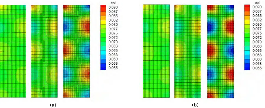
Figure 7 shows the equivalent plastic strain for the three meshes, when the applied displacement is 0.07, that is 10% of final imposed displacement. Even at this low load level, there is some plastic strain concentration, that grows when the size of finite elements diminishes. The concentration of plastic strain is larger when the ALE formulation is used, specially for mesh 3, as can be seen in Fig. 7a.

(a) (b)

Fig. 7 Equivalent plastic strain at 10% of final displacement applied to meshes 1, 2, 3, a) UL formulation;

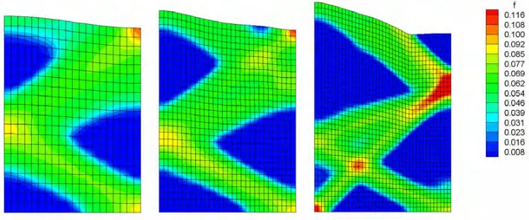
Figure 8 shows the porosity fields obtained for meshes 1, 2 and 3 using UL formulation. The results corresponding to the ALE formulation are shown in Fig. 9. It can be seen that the results for meshes 1 and 2 are very close when ALE formulation is employed. Considering mesh 3, the porosity field is highly distorted. This is probably due to the small size of the elements, that introduces the well known lack of objectivity phenomenon. For this problem, other numerical techniques, as the nonlocal approach[3] must be considered.

Fig. 8 Porosity obtained with meshes 1, 2 and 3 and UL formulation

Fig. 9 Porosity obtained with meshes 1, 2 and 3 and ALE formulation

SUMMARY AND CONCLUSIONS

The use of an ALE formulation to analyze damage problems has some advantages over the UL formulation. Considering the two cases analyzed, it can be seen that the elements in the highly damaged zone are much less distorted and, as a consequence, the change in behavior due to mesh refinement is less intense.

For the example of traction of a prismatic bar, the differences between UL and ALE results diminish together with the elements size; the same cannot be said in the case of plane strain shear bands.

ACKNOWLEDGEMENTS

We thank CAPES (project CAPES/GRICES 127/05), CNPq and PROPESQ-UFRGS for the continuous support of this research project.

REFERENCES

1. Gurson, A.L., “Continuum Theory of Ductile Rupture by Void Nucleation and Growth: Part I-Yield Criteria and Flow Rules for Porous Ductile Media,” Trans. of ASME, Journal of Engineering Materials and Technology, Vol.99, 1977, pp. 2-15.

2. Tvergaard, V., “Influence of Voids on Shear Band Instabilities Under Plane Strain Conditions,” International Journal of Fracture, Vol.17, 1981, pp.389-407.

3. César de Sá, J.M.A., Areias, P.M.A., Zheng, C., “Damage Modeling in Metal Forming Problems Using an Implicit Nonlocal Gradient Model,” Computer Methods in Applied Mechanics and Engineering, Vol.195, 2006, pp.6646-6660. 4. Hogge, M., Ponthot, J.P., and Quoirin, D., “METAFOR: Logiciel Eulérien-Lagrangien Pour l’Analyse de la Mise à Forme

et des Grandes Deformations de Matériaux,” New Advances in Computational Structural Mechanics, pp. 657-664, P. Lavadezes et al. (eds.), Giens, 1991.

5. Bittencourt, E. and Creus, G.J., “Finite Element Analysis of Three Dimensional Contact And Impact In Large Deformation Problems,” Computers and Structures, Vol.69, 1998, pp.219-234.

6. Aymone, J.L.F., Bittencourt, E. and Creus, G.J., “Simulation of 3D Metal-Forming Using an Arbitrary Lagrangian-Eulerian Finite Element Method,” Trans. of ASME, Journal of Materials Processing Technology, Vol.110, 2001, pp.218-232.

7. Chu, C.C. and Needleman, A., “Void Nucleation Effects in Biaxially Stretched Sheets,” Trans. of ASME, Journal of Engineering Materials and Technology, Vol.102, 1980, pp.249-256.

8. ABAQUS, Theory Manual v. 5.2, Hibbit, Karlsson & Sorensen, Inc., Providence, USA, 1992.

9. Cunda, L.A.B. and Creus, G.J., “A Note on Damage Analyses in Processes With Nonmonotonic Loading,” Computer Modeling and Simulation in Engineering, Vol.4, 1999, pp.300-303.

10. Tvergaard, V., “Material Failure by Void Coalescence in Localized Shear Bands,” International Journal of Solids and Structures, Vol.18, 1982, pp.659-672.

12. Belytschko, T., Liu, W.K., and Moran, B., Nonlinear Finite Elements for Continua and Structures, Wiley, 2000.

13. Cunda, L.A.B., “Gurson Model for Ductile Damage: Computational Approach and Applications” (in portuguese), Ph.D. Thesis, Universidade Federal do Rio Grande do Sul, Brazil, 2006.

14. Stainier, L., “Modélisation numérique du comportement irréversible des métaux ductiles soumis à grandes déformations avec endommagement,” (in French), Ph.D. Thesis, Université de Liège, 1996.