CHRISTOFFERSEN, CARLOS ENRIQUE. Global Modeling of Nonlinear Microwave Circuits (Under the direction of Michael B. Steer.)
by
CARLOS ENRIQUE CHRISTOFFERSEN
A dissertation submitted to the Graduate Faculty of North Carolina State University
in partial fulfillment of the requirements for the Degree of
Doctor of Philosophy
ELECTRICAL ENGINEERING
Raleigh
2000
APPROVED BY:
List of Figures vii
List of Tables xi
List of Symbols xii
List of Abbreviations xv
1 Introduction 1
1.1 Motivations and Objectives of This Study . . . 1
1.2 Review of Circuit Simulation Technology . . . 2
1.2.1 Object-Oriented Circuit Simulators . . . 5
1.3 Original Contributions . . . 6
1.4 The Global Modeling Concept . . . 8
1.5 Thesis Overview . . . 9
1.6 Publications . . . 10
1.6.1 Journals . . . 10
1.6.2 Conferences . . . 10
2 Literature Review 12 2.1 Transient Analysis of Microwave Circuits . . . 12
2.1.1 Impulse Response and Convolution . . . 13
2.1.2 Numerical Inversion of Laplace Transform Technique . 13 2.1.3 Approximations using Pole-Zero Models . . . 14
2.2 Multiresolution Analysis of Circuits . . . 16
2.2.1 Adaptive Circuit Simulation Methods . . . 16
2.2.2 Wavelets Applied to Solve Differential Equations . . . . 17
2.2.3 Spline Pseudo-Wavelet Collocation Method . . . 18
2.3.2 Trapezoidal Rule . . . 29
2.4 Parameterized Nonlinear Models . . . 29
2.5 Multitone Frequency-Domain Simulation of Nonlinear Circuits 30 2.6 Summary . . . 32
3 Generalized State Variable Reduction 33 3.1 Generalized Reduced Nonlinear Error Function Formulation . 33 3.1.1 Linear Network . . . 34
3.1.2 Nonlinear Network . . . 35
3.1.3 Error Function Formulation . . . 35
3.2 Discussion . . . 36
4 Convolution Transient Analysis 38 4.1 Introduction . . . 38
4.2 Harmonic Balance Analysis . . . 39
4.3 Formulation of the Convolution Transient . . . 40
4.3.1 Initial Operating Point . . . 41
4.4 Error Reduction Techniques . . . 42
4.4.1 Impulse Response Determination . . . 42
4.4.2 Correction of the DC Error . . . 44
4.4.3 Convolution . . . 45
4.5 Software Implementation . . . 46
4.6 Nonlinear Transmission Line . . . 47
4.7 Simulation Results and Discussion . . . 48
5 Wavelet Transient Analysis 53 5.1 Introduction . . . 53
5.2 Reduced Error Function Formulation . . . 54
5.2.1 System Expansion . . . 54
5.2.2 Initial Conditions in the State Variables . . . 58
5.2.3 Solution of the Nonlinear System Considerations . . . . 58
5.2.4 Other Transformation Types . . . 59
5.2.5 Resolution Limits . . . 59
5.3 Implementation . . . 60
5.4 Simulation Results and Discussion . . . 63
6.2 Reduced Error Function Formulation . . . 67
6.3 Implementation . . . 68
6.4 Simulation Results and Discussion . . . 70
7 Object Oriented Circuit Simulator 72 7.1 Introduction . . . 72
7.2 The Network Package . . . 74
7.3 The Analysis Classes . . . 79
7.4 Nonlinear Elements . . . 81
7.5 Example: Use of Polymorphism . . . 84
7.6 Support Libraries . . . 86
7.6.1 Solution of Sparse Linear Systems . . . 86
7.6.2 Vectors and matrices . . . 86
7.6.3 Solution of nonlinear systems . . . 87
7.6.4 Fourier transform . . . 88
7.6.5 Automatic differentiation . . . 88
7.7 Summary . . . 90
8 Modeling of Quasi-Optical Systems 92 8.1 Introduction . . . 92
8.2 Implementation of Local Reference Nodes . . . 93
8.2.1 Background . . . 93
8.2.2 Handling of Local Reference Nodes . . . 94
8.2.3 Implementation in Transim . . . 97
8.3 Integration of Electromagnetic Structures . . . 100
8.3.1 Frequency Domain and Time Domain Using Convolution100 8.3.2 Time Domain using Pole-Zero Approximations . . . 101
8.3.3 CPW Folded-Slot Active Antenna Array . . . 104
8.3.4 2x2 Grid Amplifier . . . 111
8.4 Electro-Thermal Modeling . . . 120
8.4.1 Thermal Impedance Matrix . . . 120
8.4.2 Implementation of Thermal Circuits and Elements in Transim . . . 121
8.4.3 Electrothermal Modeling of a Quasi-Optical System . . 122
9.2 Future Research . . . 131
9.2.1 The Sliding Window Scheme . . . 132
A Transim’s Graphical User Interface 134 A.1 Introduction . . . 134
A.2 The Netlist Editor . . . 134
A.3 The Analysis Window . . . 135
A.4 The Output Viewer Window . . . 135
B Object Oriented Programming Basics 138 B.1 UML diagrams . . . 140
1.1 Relation between v and i in a diode. . . 4
1.2 Relation between x and i in a diode. . . 4
1.3 Relation between x and v in a diode. . . 5
1.4 Partition of a system into spatially distributed and lumped linear circuit, nonlinear network, and thermal parts. . . 9
2.1 The scaling functionϕ(t). . . 19
2.2 The boundary scaling functionϕb(t). . . 19
2.3 The wavelet functionψ(t). . . 20
2.4 The boundary wavelet functionψb(t). . . 21
2.5 Boundary spline: η1(t). . . 23
2.6 Boundary spline: η2(t). . . 23
2.7 Boundary wavelet function: ψb0. . . 24
2.8 Boundary wavelet function: ψb1. . . 25
2.9 Partition representation of the time-invariant harmonic bal-ance method . . . 30
3.1 Network with nonlinear elements. . . 34
3.2 A quasi-optical grid. . . 37
4.1 Augmentation and compensation network . . . 43
4.2 Flow diagram of the analysis code . . . 46
4.3 Model of the nonlinear transmission line. . . 47
4.4 Complete transient response for the soliton line. . . 48
4.5 Comparison between experimental data and simulations. . . . 49
4.6 Magnitude of the harmonics of the output power. . . 50
4.7 Magnitude of the harmonics of the output power along the line. Blue is low and red is high power. . . 51
5.1 Scaling functions for L= 6. . . 54
5.2 Wavelet functions in W0 forL= 6. . . 55
5.3 Representation of the nonzero elements of the transformation matrices for L= 10 and J = 2: (a)W and (b)W0. . . 56
5.4 Linear system construction. . . 56
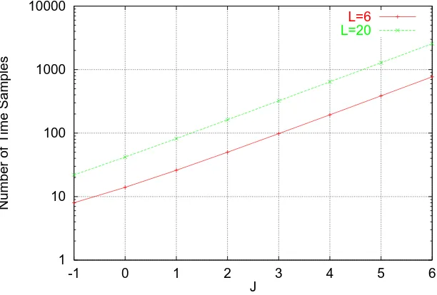
5.5 Number of time samples in the interval as a function of J for a small circuit. . . 60
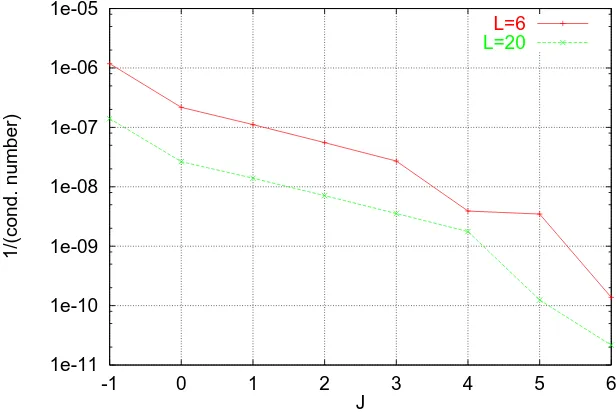
5.6 Reciprocal of the condition number ofMJ in the interval as a function of J for a small circuit. . . 61
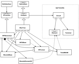
5.7 Class diagram for the wavelet-transient-based analysis in Tran-sim. . . 62
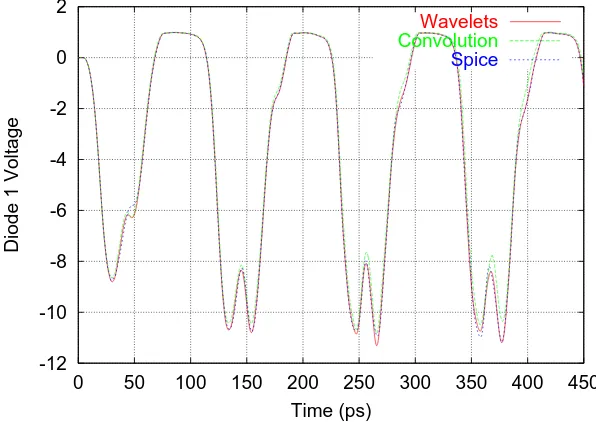
5.8 Comparison of the voltage of the diode close to the generator (diode 1). . . 64
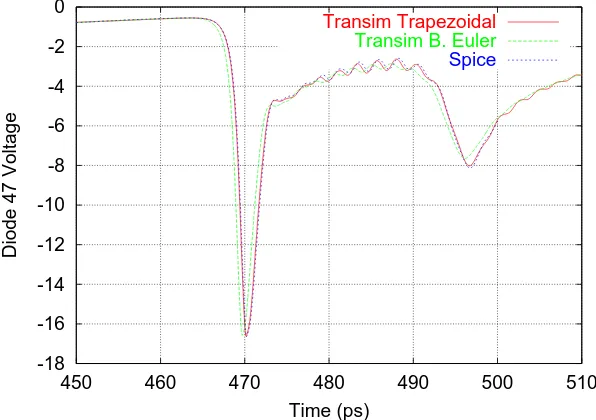
5.9 Comparison of the voltage of the diode close to the load (diode 47) of the nonlinear transmission line. . . 64
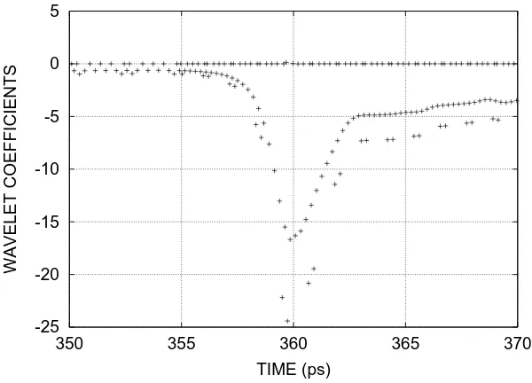
5.10 Coefficients of the state variable of diode 47. . . 65
6.1 Integration method interface. . . 69
6.2 Comparison of the voltage of the last diode. . . 70
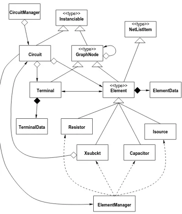
7.1 The network package is the core of the simulator. . . 75
7.2 The NetListItem class. . . 76
7.3 The Element class. . . 76
7.4 Documentation generated for an element. . . 77
7.5 The Circuit class. . . 78
7.6 The Xsubckt class. . . 79
7.7 The analysis classes. . . 80
7.8 Dependency inversion was used to make the elements indepen-dent of the analysis classes. . . 82
7.9 Class diagram for an element using generic evaluation. . . 83
7.10 Nonlinear element function evaluation in convolution transient. 85 7.11 Implementation of automatic differentiation. . . 89
8.1 Equivalent circuit of a two-port distributed element. . . 95
8.4 Illegal connection between groups. . . 97
8.5 Circuit containing an illegal element. The numbers at the nodes indicate the order in which terminals are discovered. . . 98
8.6 Collaboration diagram showing the violation detection algo-rithm. . . 99
8.7 Sample frequency-domain y parameter file. . . 101
8.8 Comparison between the original and the approximated y11 for the 2x2 grid. . . 102
8.9 Sample time-domain y parameter file. . . 103
8.10 Unit cell of the CPW antenna array. . . 105
8.11 Circuit model of the unit cell. The diamond symbol indicates a local reference node. . . 106
8.12 Effective isotropic power gain as a function of frequency. . . . 106
8.13 2x2 CPW antenna array. . . 107
8.14 2x2 CPW antenna array equivalent circuit. . . 108
8.15 Netlist for a 2x2 CPW antenna array. . . 109
8.16 Output currents for the 2x2 antenna array. . . 110
8.17 Setup for measurement characterization of the quasi-optical amplifier system. . . 111
8.18 Layout for 2x2 quasi-optical grid amplifier. . . 112
8.19 Full spectrum for output voltage. . . 113
8.20 Spectral regrowth in one of the amplifiers. . . 114
8.21 Transient response at one of the MMIC output ports using a large time step. . . 115
8.22 Zoom of the transient response at one of the MMIC output ports using a small time step. . . 116
8.23 Output transient starting with the circuit already biased. . . 117
8.24 Comparison of the steady-state output waveforms. . . 118
8.25 Transient response of one amplifier with RF excitation. . . 119
8.26 Amplifier circuit used. . . 122
8.27 Thermal circuit model for the 2x2 CPW array. . . 123
8.28 Comparison of the steady-state output voltage with and with-out thermal effects. . . 124
8.29 Steady-state temperature at the MESFET and the substrate. . 125
ture (300 K). . . 127
8.33 Transient of the substrate temperature. The temperature shown is the difference with respect to the ambient temperature (300 K).128 9.1 The sliding window scheme. . . 132
A.1 Netlist Editor window. . . 135
A.2 Analysis window. . . 136
A.3 Output Viewer window. . . 136
A.4 Plot window. . . 137
6.1 Comparison of simulation times for the soliton line . . . 71
8.1 Comparison of the simulation times for the 2 by 2 grid array . 118
<() – Real part.
ω – Angular frequency.
t – Time.
H(s) – Transfer function in the Laplace domain.
H2(I) – Sobolev space.
ϕ(t) – Scaling function.
ϕb(t) – Boundary scaling function.
Z – The set of integer numbers.
J – Wavelet subspace level.
ψ(t) – Wavelet function.
ψb(t) – Boundary wavelet function.
ψb0(t) – Boundary wavelet function.
ψb1(t) – Boundary wavelet function.
η1(t) – Boundary spline function.
η2(t) – Boundary spline function.
ˆf() – Wavelet coefficient vector of function sample vector f x(t) – Nonlinear element state variable vector.
vNL(t) – Nonlinear element port voltage vector.
iNL(t) – Nonlinear element port current vector.
nt – Number of tones.
C – Nonlinearity order.
G – Frequency-independent component of the MNAM.
C – Frequency-dependent component of the MNAM.
u – Vector of nodal unknowns and selected variables.
s – Source vector in MNAM system.
T – Incidence matrix.
ns – Number of state variables.
MSV – Frequency domain compressed impedance matrix.
mSV – Compressed impulse response impedance matrix.
WJ – Wavelet transformation matrix up to subspace level J.
WJ0 – Wavelet derivative transformation matrix up to subspace level J.
xJ – State variable vector at all collocation points.
ˆ
xJ – State variable wavelet coefficient vector.
MJ – Wavelet-expanded MNAM.
sf,J – Wavelet-expanded source vector.
Msv,J – Wavelet-expanded compressed impedance matrix.
ssv,J – Wavelet-expanded compressed source vector.
Msv – Time marching compressed impedance matrix.
ACPR – Adjacent Channel Power Regrowth. AWE – Asymptotic Waveform Evaluation. BE – Backward Euler.
CAE – Computer Aided Engineering. CPW – Coplanar Waveguide.
DFT – Direct Fourier Transform. EM – Electro Magnetic.
FDTD – Finite Difference Time Domain. FFT – Fast Fourier Transform.
HB – Harmonic Balance.
I-FFT – Inverse Fast Fourier Transform. IRC – Impulse Response and Convolution. KCL – Kirchoff Current Law.
LRG – Local Reference Group. LRN – Local Reference Node.
MMIC – Monolithic Microwave Integrated Circuit. MNAM– Modified Nodal Admittance Matrix. MRA – Multiresolution Analysis.
NILT – Numerical Inverse Laplace Transform. NLTL – Nonlinear Transmission Line.
ODE – Ordinary Differential Equation. OO – Object Oriented.
PDE – Partial Differential Equation. QO – Quasi-Optical.
RF – Radio Frequency.
RLCG – Resistor, Inductor, Capacitor, Conductor. STL – Standard Template Library.
Introduction
1.1
Motivations and Objectives of This Study
The almost overwhelming use of the circuit abstraction in electronic engi-neering has enabled the design of surprisingly complex systems [1]. There are three important reasons for simulating electronic circuits: to understand the physics of a complex system of interacting elements; to test new con-cepts; and to optimize designs. Millimeter-wave circuits are becoming ever more commercially and militarily viable and, coupled with large scale pro-duction, design practices must evolve to be more sophisticated in order to handle more complex relationships between constituent elements. Also, as the frequency of RF circuits extends beyond a gigahertz to tens and hun-dreds of gigahertz, device and circuit dimensions become large with respect to wavelength and the three dimensional electro magnetic (EM) environ-ment becomes more significant. If reliable, high yielding, optimized designs of microwave and millimeter-wave circuits are to be achieved, the interre-lated effects of the EM field, the linear and nonlinear circuit elements and the thermal subsystem must be self-consistently modeled.
This work attempts to develop a unified circuit view for integrating linear and nonlinear devices with electromagnetic and thermal effects. The basic idea is to convert the EM and thermal problems into circuit abstraction. An-other objective of this study is to develop efficient circuit analysis techniques that can be used to simulate the whole system.
In this thesis, a general state variable reduction error function formu-lation is presented. This formuformu-lation is numerically efficient and allows a
very flexible and convenient software implementation in a circuit simulator. Several circuit transient analysis methods are derived from this formulation; based on convolution, wavelets and time-marching schemes. It is also shown that the harmonic balance analysis developed in [2] is a particular case of the general state variable error function formulation. The state-variable-based convolution analysis was used here to perform a transient simulation of a 47-section nonlinear transmission line (NLTL) with frequency-dependent at-tenuation for the first time. The combination of the state variable reduction developed here with time marching schemes achieves more than an order of magnitude improvement in simulation speed comparing with traditional circuit simulation methods.
All these developments are implemented in a circuit simulator program, called Transim. The novel techniques used in the design of this program are described. Two quasi-optical power amplifier arrays are modeled and simulated. The results for electrical-only and simultaneous thermal-electrical simulations are presented and commented.
1.2
Review of Circuit Simulation Technology
The most widespread [3] method of nonlinear circuit analysis is time-domain analysis (also called transient analysis) using programs like Spice. Such pro-grams use numerical integration to determine the circuit response at one instance of time given the circuit’s response at a previous instance of time. The success of Spice is that the associated modeling approach works ex-tremely well. In Spice the circuit model is discretized in time and merged with a Newton iteration step to form what is called an associated discrete model. This associated discrete model is linear and so the mathematical for-mulation and solution is linear. If an error, such as a Kirchoff’s current law error, is detected the associated model is updated and solved again. It is not obvious that this is a better way of solving the circuit problem than solv-ing the coupled nonlinear integro-differential problem directly as would be required without introducing the associated model. However it is extremely robust and numerically efficient.
Some are ideally suited to particular applications. An example is harmonic balance (HB) analysis of RF and microwave circuits. Harmonic balance dif-fers [4] from traditional transient analysis in two fundamental ways. These differences allow harmonic balance to compute periodic and quasi-periodic solutions directly and in certain circumstances give the method significant advantages in terms of accuracy and efficiency. The first difference between harmonic balance and transient analysis is that harmonic balance uses a lin-ear combination of sinusoids to build the solution. Thus, it approximates naturally the periodic and quasi-periodic signals found in a steady-state re-sponse. Harmonic balance also differs from traditional time domain methods in that time domain simulators represent waveforms as a collection of sam-ples whereas harmonic balance represents them using the coefficients of the sinusoids.
Rizzoli [5] proposed a state variable approach in the HB simulation con-text (described in Section 2.4) which provides great flexibility for the design of nonlinear device models. The state variables can be chosen to achieve robust numerical characteristics. As an example we present a parameterized diode model as described in [5]. The full model includes capacitances and nonlinear resistance, but here a simple case is shown for didactic purposes. The conventional current equation for the diode is
i(t) =Is(exp(αv(t))−1)
and, based on previous work [5], the parametric model is as follows
v(t) =
(
x(t) if x(t)≤V1
V1+α1 ln(1 +α(x(t)−V1)) if x(t)> V1
i(t) =
(
Is(exp(αx(t))−1) if x(t)≤V1
Isexp(αV1)(1 +α(x(t)−V1))−Is if x(t)> V1
where V1 is some threshold value.
−1 −0.8 −0.6 −0.4 −0.2 0 0.2 0.4 0.6 0.8 1 −0.1
0 0.1 0.2 0.3 0.4 0.5 0.6
I (A)
V (V)
Figure 1.1: Relation between v and i in a diode.
−1 −0.5 0 0.5 1 1.5 2 2.5 −0.1
0 0.1 0.2 0.3 0.4 0.5 0.6
X
I (A)
−1 −0.5 0 0.5 1 1.5 2 2.5 −1
−0.8 −0.6 −0.4 −0.2 0 0.2 0.4 0.6 0.8 1
X
V (V)
Figure 1.3: Relation between x and v in a diode.
change is generally limited so that there can be no more than 10% change in i or v. The possibility of large changes is eliminated through the use of parameterization which ensures smooth, well behaved current, voltage and error function variations when the state variable is updated. Thus the i–x
and v–x functions are well behaved and thus circuit analysis via nonlinear iterations is also well behaved. See Figures 1.2 and 1.3.
One of the most significant developments relevant to microwave computer aided engineering is the rise of object oriented design practice. In the last years, some circuit simulators have been designed usingobject oriented (OO) techniques. A review of the key developments follows.
1.2.1
Object-Oriented Circuit Simulators
APLAC1 [6, 7] is a significant achievement in the development of
object-oriented circuit simulators with the object orientation implemented in the standard C language using macros. The most important feature of APLAC is that every circuit element is modeled internally using independent and voltage-controlled current sources. Since all models in APLAC are eventu-ally mapped to current sources, the simple nodal linear DC analysis,Gu=j,
is all that is required to realize nonlinear DC, AC, transient and harmonic balance analyses. HereG,uandjdenote conductance matrix, nodal voltages and the independent source currents, respectively. The cost of this approach is reduced speed. In part this is because the C language is not optimal for OO applications but also because the high level of abstraction intro-duces overhead. However the objective of providing great functionality to enable experimentation with new element types and analysis techniques was achieved. The current version of the program incorporates many advanced features including electro-thermal analysis and is commercially available.
Other OO circuit simulators are CODECS [8], ACS2 [9] and Sframe [10]
and these adopted a common interface for all the circuit elements. In this way, all the code related to one element is separated from the rest of the program. In other words, the main program does not have dependencies on individual elements. The result is that the programming effort required to add new elements and algorithms is greatly reduced. ACS and Sframe are written in C++ and among other features, they both allow one element to be composed of other basic elements. The underlying algorithms in ACS are the same as those in Spice. As well as the flexibility introduced by the OO design there are memory savings in storing the circuit.
Sframe incorporates several novel features including automatic differen-tiation. In this simulator C++ is used as the circuit description language rather than, say, a Spice netlist. This arrangement yields a level of flexibility difficult to achieve using a netlist parser or graphical interface. On the other hand, the netlist must be compiled and the simulator linked for each circuit, and the user must be aware of the subtle details of the C++ syntax.
Other considerations about the OO design of circuit simulators are pre-sented in [11].
1.3
Original Contributions
The simulator engine of the pre-existing Transim simulator program [2] was re-designed and coded from scratch using object oriented techniques. Only the parser and the output routines from the original program were kept, and they had been significantly modified to work with the new simulator engine and support new features. One of the outstanding new features is thegeneric
element evaluation mechanism, described in Section 7.4. No other circuit sim-ulator provides the same level of flexibility for the addition of new nonlinear device models and circuit analysis algorithms. Transim also supports the lo-cal reference node concept [12]. The conventional nodal specification enables circuit elements to be connected in any possible combination and only one reference node (commonly called the global reference node or simply ground) is used. With spatially distributed circuits it is possible to make non-physical connections such as connecting a non-spatially distributed element, say a re-sistor, across two physically separated (relative to the wavelength) parts of the circuit, e.g. the opposite ends of a transmission line. The local reference concept (described in Section 8.2) avoids this kind of problem and therefore is fundamental for the analysis of spatially distributed circuits as well as for simultaneous thermal-electrical simulations.
Another original contribution is the circuit formulation of Chapter 3, which was developed as a generalization of the harmonic balance method presented by the author in [2]. All the nonlinear circuit analysis techniques presented in this thesis are derived from the generic formulation in Chapter 3. This formulation provides a tool for the derivation of new circuit analysis techniques. It uses Rizzoli’s state variable concept discussed in Section 1.2 and thus inherits the associated advantages of this approach. The number of nonlinear unknowns resulting from our formulation is generally much smaller than the number of unknowns in conventional circuit analysis.
The convolution transient method developed by Ozkar in [13] was en-hanced and re-implemented more efficiently in the newly designed Transim (Chapter 4). Convolution transient provides modeling of frequency-defined network elements with more accuraccy than other methods, but it will be shown that it is useful when the number of time steps to be simulated is not very large. The implementation of this circuit analysis technique was the first chronologically and allowed the transient simulation for the first time of a NLTL considering frequency-dependent attenuation (Section 4.7) and, also for the first time, the transient simulation of a quasi-optical grid amplifier (Section 8.3.4).
nonlinear circuit simulator developed to date. The simulation examples us-ing the NLTL and the quasi-optical (QO) grid amplifier presented here are the most complex circuits ever simulated using wavelets. Nevertheless, as it will be shown, this circuit analysis technique requires more research to become efficient.
The state variable transient analysis based on time marching integration methods (Chapter 6), both formulation and implementation in Transim is original from this thesis. It is shown that this transient analysis offers more than an order of magnitude reduction (and it has the potential for even better performance) in the transient simulation time compared with Spice for some circuits. When combined with pole-zero modeling of EM structures, the simulations of QO systems using the method of Chapter 6 are several orders of magnitude faster than the simulations using convolution transient. Therefore, this is the preferred circuit analysis method if accurate pole-zero models for QO are available.
Other contributions include the integration of thermal circuit elements based on theLeeds’ thermal impedance matrix model to enable electro-thermal simulations in Transim (Section 8.4). This was a joint effort with Dr. William Batty of Leeds University, in the UK. Also the combination and the actual coding in Transim of the frequency spectrum generation technique of Section 2.5 with the frequency mapping technique in harmonic balance to allow the simulation of spectral regrowth using HB.
1.4
The Global Modeling Concept
LINEAR NETWORK CIRCUIT
DISTRIBUTED SPATIALLY
CIRCUIT DISTRIBUTED
CIRCUIT NETWORK NONLINEAR SPATIALLY LINEAR
THERMAL NETWORK
Figure 1.4: Partition of a system into spatially distributed and lumped linear circuit, nonlinear network, and thermal parts.
modeled independently and connected to form a thermal circuit. Note that the link between the electrical and thermal parts is through the nonlinear elements. This is so because the electrical power dissipation is always a non-linear process. The spatially distributed circuit could certainly be directly connected to the nonlinear devices and this is consistent with this model.
The analysis strategy described in Chapter 3 shows that the complete nonlinear system can be simulated by knowing only the state of the nonlinear network. However, since the thermal subsystem is often nonlinear, part of it must be embedded into the nonlinear network to achieve this.
1.5
Thesis Overview
The second Chapter is dedicated to the literature review. Chapter 3 de-scribes the generalized state variable analysis used in this work to analyze circuits and systems. Then there is one Chapter for each concrete circuit analysis derived from the general approach. Each method is formulated, implemented and tested. The pros and cons of each method are discussed. Convolution transient is treated in Chapter 4, wavelet transient in Chapter 5 and timemarching transient in Chapter 6. The system used for testing is a nonlinear transmission line described in Section 4.6.
were used in its design.
Chapter 8 presents modeling issues specific to quasi-optical systems, in-cluding the need for local reference nodes, the modeling of electromagnetic structures and thermal effects. Two different structures are simulated using different methods and the results are commented.
Finally, Chapter 8 contains general conclusions and ideas for continuation of this research.
The first appendix describes the Graphical User Interface (GUI) devel-oped to make the use of Transim easier. The second presents a very short and incomplete introduction to object oriented programming that might be nevertheless useful to understand Chapter 7.
1.6
Publications
1.6.1
Journals
1. C. E. Christoffersen, U. A. Mughal and M. B. Steer, “Object Ori-ented Microwave Circuit Simulation,” Int. J. of RF and Microwave Computer-Aided Engineering, Vol. 10, Issue 3, 2000, pp. 164–182.
2. C. E. Christoffersen, M. Ozkar, M. B. Steer, M. G. Case and M. Rod-well, “State variable-based transient analysis using convolution,” IEEE Transactions on Microwave Theory and Techniques, Vol. 47, June 1999, pp. 882–889.
3. C. E. Christoffersen and M. B. Steer “Implementation of the local ref-erence concept for spatially distributed circuits,” Int. J. of RF and Microwave Computer-Aided Eng., vol. 9, No. 5, 1999, pp. 376–384.
4. M. B. Steer, J. F. Harvey, J. W. Mink, M. N. Abdulla, C. E. Christof-fersen, H. M. Gutierrez, P. L. Heron, C. W. Hicks, A. I. Khalil, U. A. Mughal, S. Nakazawa, T. W. Nuteson, J. Patwardhan, S. G. Skaggs, M. A. Summers, S. Wang, and A. B. Yakovlev, “Global modeling of spatially distributed microwave and millimeter-wave systems,” IEEE Trans. Microwave Theory Techniques, June 1999, pp. 830–839.
1.6.2
Conferences
“Transient analysis of a spatial power combining amplifier”,1999 IEEE MTT-S Int. Microwave Symp. Dig., June 1999, pp. 791–794.
2. W. Batty, C. E. Christoffersen, S. David, A. J. Panks, R. G. Johnson, C. M. Snowden and M. B. Steer, “Predictive microwave device design by coupled electro-thermal simulation based on a fully physical thermal model,” EDMO 2000, Glasgow UK, November 2000.
3. W. Batty, C. E. Christoffersen, S. David, A. J. Panks, R. G. Johnson, C. M. Snowden and M. B. Steer, “Steady-state and transient electro-thermal simulation of power devices and circuits based on a fully phys-ical thermal model,” THERMINIC 2000 Digest, Budapest, September 2000.
4. H. Gutierrez, C. E. Christoffersen and M. B. Steer, “An integrated en-vironment for the simulation of electrical, thermal and electromagnetic interactions in high-performance integrated circuits,” Proc. IEEE 6 th Topical Meeting on Electrical Performance of Electronic Packaging, Sept. 1999, pp. 217–220.
Literature Review
First, microwave circuit transient analysis techniques are reviewed. These are relevant to the new techniques proposed in the following chapters. Section 2.2 is dedicated to the application of wavelets to the simulation of circuits and a description of the wavelet basis functions used to implement the method in Chapter 5. Section 2.3 briefly presents a review of time marching integration methods. We will use these methods to derive a new type of circuit analysis in Chapter 6. Section 2.4 presents the state variable variable approach adopted here to analyze nonlinear circuits. Section 2.5 is dedicated to the review of a method to produce all the intermodulation products present in a circuit given certain spectrum of the exciting tones. This novel technique technique was applied combined with harmonic balance (possibly for the first time) in Transim to evaluate spectral regrowth in power combiners.
2.1
Transient Analysis of Microwave Circuits
Distributed linear microwave circuits are described by frequency-dependent network parameters and only a few methods are available to accommodate these circuits in transient simulation. These methods include Impulse Re-sponse and Convolution (IRC), Laplace Inversion and the approximation of network functions using pole-zero models, which be subdivided in Asymp-totic Waveform Evaluation (AWE) and Interpolation Methods. We briefly describe these methods in the following sections.
2.1.1
Impulse Response and Convolution
One of the first implementations of IRC to distributed microwave circuits was by Djordjevic and Sarkar [14] in 1987. Since that time there have been several efforts to reduce the significant aliasing errors that result from the Inverse Fast Fourier Transform (I-FFT) operation.
Minimization of aliasing in the I-FFT requires that the imaginary part of the frequency response be zero at the maximum frequency. Low pass filtering has been used to achieve this [15]. The introduction of a small time delay also achieves this result with presumably less distortion [16]. Insertion of an augmentation network in the linear network at the interface with the non-linear network achieves the same result for special types of circuits [17]. The effect of the augmentation network is compensated in the nonlinear iteration scheme. This, however, is not a general technique. It is also important to limit the length of the impulse response to reduce memory requirements and the resistive augmentation achieves this result [17]. Augmentation is also effectively achieved using scattering (S) parameters [18], where the reference impedance effectively dampens multiple reflections.
Distributed networks are characterized partly by reflections so that an impulse response tends to have regions of low value between regions of rapid change. In this case thresholding greatly reduces the number of impulse response discretizations that need to be retained [17]. In high speed digi-tal interconnect circuitry this can reduce the number of significant impulse responses by a factor of 10 to 100, depending on the desired accuracy [17].
Convolution as generally implemented uses a rectangular integration scheme (essentially an impulse response is treated as being constant in a time step interval). P. Stenius et al. [19] developed a trapezoidal form of the convolu-tion integraconvolu-tion which should have superior convergence properties than the previous block integration.
2.1.2
Numerical Inversion of Laplace Transform
Tech-nique
for the other parts of the response. Laplace techniques suffer from the series approximations and the nonlinear iterations involved. If only Y(jω) is avail-able (e.g. through measurements) the I-FFT must be used instead of the NILT. The advantages and the limitations of the Inverse Laplace Methods are discussed in detail in [20].
2.1.3
Approximations using Pole-Zero Models
Asymptotic Waveform Evaluation
The frequency dependent network parameters can be modeled using fre-quency independent primitives (resistors, inductors and capacitors) if a ratio-nal polynomial transfer function is fitted to the network parameters. In prac-tice, this procedure results in an impossibly large circuit. The AWE method addresses this problem by reducing the dimension of the rational polynomial while minimizing distortion [21,22]. This method works well for interconnects in digital systems and lower frequency microwave circuits [23, 24]. However, higher frequency circuits can only be modeled approximately using AWE due to the infinite number of poles and zeros of such a circuit.
Most of the AWE methods use the Pad´e approximation and this and other approximations used can have stability problems [21].
Interpolation Methods
Besides AWE, there are other techniques to approximate network parameters using a rational polynomial transfer function. Here we will briefly summarize the method that will be used in Section 8.3.2. The procedure in detail was presented by Beyene et al. in [25].
A network functionY(s) can be approximated by the rational function
H(s) = q0+q1s+q2s
2+. . .+q
ξsξ
1 +r1s+r2s2+. . .+rϑsϑ
, (2.1)
Let ωmin and ωmax be the lowest and highest frequencies of the data
sample set, respectively. The first step in this method is to normalize and shift frequency points to map [ωmin, ωmax] onto [−1,1].
Then, the real part of the original functionY(s) is fitted to the real part of the rational polynomial function H(s), leading to the following form
<(H(s)) = C(s)
D(s) =
c0+c1s2+c2s4+. . .+cξs2ξ
1 +d1s2+d2s4+. . .+dϑs2ϑ
(2.2)
Let yi be
yi =Y(jωi) (2.3)
i.e., the value of the network function ats=jωi. Then, from Equation (2.2),
making <(H(jωi)) =<(yi),
C(jωi)−D(jωi)<(yi) = 0 (2.4)
A linear system of equations is built by applying Equation (2.4) at each frequency sample. There are some considerations about how many sample points are necessary. At leastn=ξ+ϑ+1 are needed. If there are more sam-ples, [25] proposes to use the method of averages [26]. Briefly, the equations (more than n) are arranged inngroups, and the equations in each group are added so the final system is square. Note that then the aproximation will no longer be an interpolation.
The linear system of equations is solved for the polynomial coefficients. The authors of [25] suggest using QR decomposition instead of Gaussian elimination in order to avoid the growth factor present in Gaussian elimina-tion. They also state that for this ill-conditioned problem, the orthogonal method gives an added measure of reliability. The frequency normalization also helps to reduce the ill conditioning of the matrix.
Once the coefficients di are known, it is possible to extract the poles of
the real part by calculating the roots ofD(s). Only the poles in the left-hand plane are kept and the rest is discarded. Pure-imaginary complex conjugate poles are taken only if they are double. The extracted poles are denoted pi.
The solution for a given pair ξ, ϑ may not be acceptable. If so, a new order of approximation is selected and the previous calculation repeated.
WriteH(s) in (2.1) in pole-residue form
H(s) =k∞+
ϑ0
X
i=1
ki
s−pi
where ϑ0 ≤ ϑ and ϑ−ϑ0 is the number of rejected purely imaginary poles.
ki denotes the residues and k∞ represents any direct coupling between input
and output. From this form, it is possible to formulate another linear system to find the residues and finally obtain the approximating rational function.
2.2
Multiresolution Analysis of Circuits
In this section we review methods for the simulation of circuits with nonuni-form meshes. We concentrate in techniques based on wavelets. Since the simulation of circuits consist in solving coupled algebraic and ordinary dif-ferential equations (ODEs), Section 2.2.2 reviews wavelet methods applied to the solution of differential equations. One particular method is reviewed in section 2.2.3. The implementation of the wavelet transient analysis presented in Chapter 5 is based on this.
2.2.1
Adaptive Circuit Simulation Methods
Adaptive circuit simulation methods attempt to adapt the position and the number of time samples of the different circuit variables in order to save computation time and memory. The difference between this approach and conventional time-marching methods is that the position of time samples must not necessarily be shared by all circuit variables. One natural ap-proach to achieve this is to use wavelets. Wavelet methods for the solution of PDEs have direct application in the analysis of electromagnetic structures and in the modeling of semiconductor devices. The transient analysis of general circuits involves the solution of a set of nonlinear coupled algebraic
and ODEs. Methods developed with PDEs in mind can be modified to solve circuit equations, however its use is not widespread.
method was shown to speed up the convolution operation by around two to six times comparing with the conventional FFT method.
Other applications include, but they are not limited to, analysis of tran-sient signals in circuits ( [29,30] are some examples) and the analysis of linear time-variant electrical networks [31].
Zhou et al. presented the pseudo-wavelet collocation method developed in [32] modified to solve linear ordinary differential equations (ODEs) in [33] and nonlinear ODEs in [34]. The same method and examples were presented with some more detail using the boundary wavelets proposed in [35] in [36] and [37]. This method is described in Section 2.2.3.
Wenzleret. al [38] propose an adaptive algorithm based on interpolating splines. The interpolation points are adjusted to minimize the error. This method does not use wavelets.
2.2.2
Wavelets Applied to Solve Differential Equations
Wavelets offer a means of approximating functions that allows selective grid refinement [39]. If regions of an image or a signal have exceptionally large variations, one need only store a set of coefficients, determined by function values in the neighborhoods of those regions, in order to reproduce these variations accurately. In this way, one can have approximations of functions in terms of a basis that has spatially varying resolution. This approach reduces the memory storage required to represent functions and may be used for data compression.
Wavelet approximations [32] have attracted much attention as a poten-tially efficient numerical technique for solving partial differential equations. Because of their advantageous properties of localizations in both space and frequency domains, wavelets seem to be great candidate for adaptive and multiresolution schemes to obtain solutions which vary dramatically both in space and time and develop singularities. On one hand, these methods allow one to design methods of arbitrarily high order, and on the other hand they display a local behavior. For introductory material on wavelets the reader is referred to [40, 41].
must verify the equation exactly at some collocation points.
2.2.3
Spline Pseudo-Wavelet Collocation Method
This method is of special interest since it has been applied to circuit transient simulation by Zhou et al. in [33, 36]. The Transim implementation of the wavelet transient formulation presented in Chapter 5 is also based on this.
Scaling Spline Wavelet Functions
First a short introduction to multiresolution analysis (MRA) is presented based on the material in [32]. Refer to the original article for mathematical proofs. For simplicity, we will use the term ‘wavelet’ in this discussion with the understanding that it is different from the usual wavelet which has a non vanishing moment.
LetI denote a finite intervalI = [0, L],Lis a positive integer, L >4 and
H2(I) and H2
0(I) denote the following two Sobolev spaces:
H2(I) = {f(t), t∈I| kf(i) k2<∞, i= 0,1,2} (2.6)
H02(I) = {f(t)∈H2(I)|f(0) =f0(0) =f(L) =f0(L) = 0} (2.7)
H2
0(I) is a Hilbert space equipped with inner product
hf, gi=
Z
I
f00(t)g00(t)dt (2.8)
thus
|||f|||=qhf, fi (2.9) provides a norm for H2
0(I).
Approximation of a Function in H2 0(I)
To generate an MRA for the Sobolev space H2
0(I), we consider two scaling
functions; an interior scaling function ϕ(t) and a boundary scaling function
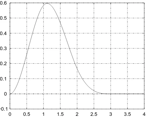
ϕb(t) (see Figs. 2.1 and 2.2)
ϕ(t) = N4(t) =
1 6 4 X j=0 4 j !
(−1)j(t−j)3+
ϕb(t) =
3 2t 2 +− 11 12t 3 ++ 3
2(t−1)
3 +−
3
4(t−2)
0 0.1 0.2 0.3 0.4 0.5 0.6 0.7
0 0.5 1 1.5 2 2.5 3 3.5 4
Figure 2.1: The scaling function ϕ(t).
−0.1 0 0.1 0.2 0.3 0.4 0.5 0.6
0 0.5 1 1.5 2 2.5 3 3.5 4
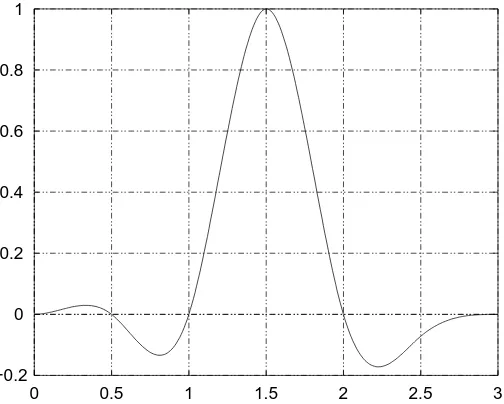
−0.2 0 0.2 0.4 0.6 0.8 1
0 0.5 1 1.5 2 2.5 3
Figure 2.3: The wavelet function ψ(t).
N4(t) is the fourth-order B-spline and for any real numbern,
xn+ =
(
xn if x≥ 0 0 otherwise
For any j, k ∈Z, we define
ϕj,k(t) = ϕ(2jt−k)
ϕb,j(t) = ϕb(2jt)
and let Vj be
Vj = span{ϕj,k(t)|ϕb,j(t), ϕb,j(L−t) : 0≤k ≤2jL−4} (2.10)
Let Vj, j ∈ Z+ be the linear span of (2.10). Then Vj forms an MRA in
H02(I) equipped with norm, Equation (2.9), and for eachj,{ϕj,k(t), ϕb,j(t), ϕb,j(L−
t)} is a basis of Vj.
To construct a wavelet decomposition of Sobolev space H2
0(I) under the
inner product of Equation (2.8), we consider the following two wavelet func-tions (see Figs. 2.3 and 2.4)
ψ(t) = −3
7ϕ(2t) + 12
7 ϕ(2t−1)− 3
7ϕ(2t−2)∈V1
ψb(t) =
24
13ϕb(2t)− 6
−0.2 0 0.2 0.4 0.6 0.8 1 1.2
0 0.5 1 1.5 2 2.5 3
Figure 2.4: The boundary wavelet function ψb(t).
It can be verified that both ψ(t) andψb(t) belong to V1 and
ψ(n) =ψb(n) = 0 for alln∈Z
Now define
ψj,k(t) = ψ(2jt−k)
ψb,jl (t) = ψb(2jt)
ψb,jr (t) = ψb(2j(L−t))
where j ≥ 0, k = 0, . . . , nj −3 and nj = 2jL. For simplicity, we will adopt
the following notation
ψj,−1(t) =ψlb,j(t)
ψj,nj−2(t) =ψ
r b,j(t)
so, whenk =−1 ornj−2, wavelet functionsψj,kwill denote the two boundary
wavelet functions, which can not be obtained by translating and dilatingψ(t). Finally, for each j ≥0 define
The Wj, j ≥ 0 as defined in Equation (2.11) is the orthogonal complement
of Vj in Vj+1 under the inner product of Equation (2.8). Therefore,
Wj ⊥ Wj+1, j ∈Z+
H02(I) = V0 M
j∈Z+
Wj
where the symbol⊥indicates orthogonality under the inner product of Equa-tion (2.8) and Vj+1 = Vj
L
Wj indicates Vj ⊥ Wj and Vj+1 = Vj+Wj. As
a consequence of this, any function f(t) ∈ H02(I) can be approximated as closely as needed by a function fj(t) ∈ Vj = V0 ⊕W0 ⊕. . .⊕Wj−1 for a
sufficiently large j, and fj(t) has a unique orthogonal decomposition
fj(t) =f0+g0+. . .+gj−1 (2.12)
where f0 ∈V0 and gi ∈Wi, 0≤ i≤j −1.
Approximation of a Function in H2(I)
Consider the following two splines (Figs. 2.5 and 2.6)
η1(t) = (1−t)2+
η2(t) = 2t+−3t2++
7 6t
3 +−
4
3(t−1)
2 ++
1
6(t−2)
3 +
For any function f(t) ∈ H2(I), we can define the following interpolating
spline Ib,jf(t),j ≥0, expected to approximate the non homogeneities of the
function f(t) at the boundaries.
Ib,jf(t) =α1η1(2jt) +α2η2(2jt) +α3η2(2j(L−t)) +α4η1(2j(L−t))
The coefficients α1, α2,α3,α4, must be chosen such that
Ib,jf(0) = f(0)
Ib,jf(L) = f(L)
(Ib,jf)0(0) = f0(0)
(Ib,jf)0(L) = f0(L)
0 0.2 0.4 0.6 0.8 1
0 0.2 0.4 0.6 0.8 1 1.2 1.4 1.6 1.8 2
Figure 2.5: Boundary spline: η1(t).
0 0.05 0.1 0.15 0.2 0.25 0.3 0.35 0.4
0 0.2 0.4 0.6 0.8 1 1.2 1.4 1.6 1.8 2
−0.4 −0.2 0 0.2 0.4 0.6 0.8 1 1.2
0 0.5 1 1.5 2 2.5 3
Figure 2.7: Boundary wavelet function: ψb0.
Now we havef(t)−Ib,jf(t)∈H02(I) and the decomposition of (2.12) can
be applied. Finally, for any function f(t) ∈ H2(I), we can find a function
fj(t) in the form of
fj(t) =Ib,jf(t) +f0 +g0+. . .+gj−1 (2.13)
which approximates f(t) as closely as needed provided thatjis large enough.
Not-a-Knot Conditions
In many applications, the solutions vary dramatically near the boundary, and the finite difference approximation suggested in the previous section could result in large errors. To overcome this problem, [32] proposes that Ib,jf(t)
agrees with f(t) at one additional point near each boundary. Reference [35] also proposes the following modifications. The boundary wavelet, ψb, is
replaced with (Figs. 2.7 and 2.8) and
ψb0(t) = −
56
99(ψ0,−1(t) + 14ψ0,−2(t))
ψb1(t) =
182
181(ψ(t) + 1
13(ψ0,−1(t) +ψ0,−2(t)))
where ψ0,−1(t) = ψ(t+ 1) and ψ0,−2(t) = ψ(t + 2). They also consider a
−0.2 0 0.2 0.4 0.6 0.8 1
0 0.5 1 1.5 2 2.5 3
Figure 2.8: Boundary wavelet function: ψb1.
the extra boundary functions. First, the scaling space V0 and wavelet space
Wj are redefined. For any j, k ∈Z, we have
ϕ0,k(t) = ϕ(t−k), 0≤k ≤L−4 (2.14)
ϕ0,−3(t) = η1(t) (2.15)
ϕ0,−2(t) = η2(t) (2.16)
ϕ0,−1(t) = ϕb(t) (2.17)
ϕ0,L−3(t) = ϕb(L−t) (2.18)
ϕ0,L−2(t) = η2(L−t) (2.19)
ϕ0,L−1(t) = η1(L−t) (2.20)
and
ψj,k(t) = ψ(2jt−k) j ≤0, k= 1,2, . . . , nj −4
ψj,−1(t) = ψb0(2jt)
ψj,0(t) = ψb1(2jt)
ψj,nj−3(t) = ψb1(2
j(L−t))
ψj,nj−2(t) = ψb0(2
j(L−t))
The new spaces V0 and Wj are then
Wj = span{ψj,k(t)| −1≤k≤nj−2, nj = 2jL} (2.22)
It can be checked that dimV0 = L+ 3 and dimWj = nj. The collocation
points are
T(−1) =
0,1
2,1,2, . . . , L−1, L− 1 2, L
=nx(k−1)oL+3
k=1 (2.23)
for V0, and
T(j) =
(
1 2j+2,
3 2j+1, . . . ,
2k+ 3
2j+1 , . . . , L−
3
2j+1, L−
1 2j+2
)
=nx(kj)onj−2
k=−1
(2.24) The modification on the boundary scaling functions partially destroys the orthogonality of the bases in Equations (2.15) to (2.20) with respect to the wavelet spaces. However, it can still be proven [35] that {ψj,k(t)} forms a
hierarchical basis function over the collocation points in (2.23)–(2.24). Summarizing, for any function f(t) ∈ H2(I), we have an approximate
function fJ(t) in the form of
fJ(t) =f0+g0+g1+. . .+gJ (2.25)
where f0 ∈V0, gj ∈Wj and 0≤j ≤J.
Application to the Numerical Solution of ODEs
The MRA just described is now applied to solve ODEs. Consider the follow-ing system of nonlinear differential equations:
( dx
dt =f(t,x)
x(0) = xt0 (2.26)
wherex(t) is an unknown vector function defined in a finite intervalI = [0, L],
L >4 andf(t,x) is a given nonlinear function. A scaling operation is applied to I to cover any interval.
LetˆxJ be the vector with the wavelet coefficients of x(t):
ˆ
xJ = (ˆx−1,−3, . . . ,xˆ−1,L−1,
ˆ
x0,−1, . . . ,xˆ0,n0−2,
ˆ
and will be determined by satisfying interpolating conditions at the colloca-tion points. Each component xi(t) of x(t) in Equation (2.26) is replaced by
its wavelet expansion form at each collocation point. Therefore we obtain the following nonlinear algebraic system
AˆxJ =ˆf(ˆxJ) (2.27)
where Ais a constant matrix that performs the derivative operation andˆf() is a nonlinear vector function.
The method to solve differential equations just described provides a uni-form error distribution on the interval [33]. By this property, large time steps can be used without introducing significant phase shifting between the approximate and exact solutions. The minimization of the error over an in-terval is the significant departure from conventional transient analysis where error is minimized at one time point at a time.
Adaptive Techniques
In wavelet analysis, computations are carried out from lower subspaces to higher ones. If the wavelet coefficients at the highest subspace level are negligible, then stop, otherwise recalculate using an additional level [33]. The same reference remarks that even in the same subspace level, there is no need to keep all the coefficients, but only the coefficients where the tolerance has not been satisfied. Reference [34] proposes the application of time windowing, a well-known technique also used in waveform relaxation [43]. Then, the original interval is divided into sub-intervals, and the method is applied using different resolutions in each time window.
Iterative Scheme to Solve the Nonlinear Equations
Zhou et al. [34] propose to solve the resulting system of algebraic nonlinear equations using the following fixed-point scheme. Derived from Equation (2.27),
ˆ
x(k+1) =ˆxk−ρAxˆk−ˆf(xˆk) (2.28) where 0 < ρ < 1 is a relaxation factor determined by a one-dimensional search at each iterative step. References [34, 37] recommend the iteration scheme of Equation (2.28) since it is a convergent scheme. However, [37] com-ments that depending on the initial guess ˆx0 of the coefficients, the scheme
2.3
Numerical Integration Using Time
March-ing Methods
The most widespread method of nonlinear circuit analysis is time-domain analysis using numerical integration to determine the circuit response at one instance of time given the circuit’s response at a previous instance of time. In this section we review some of the numerical integration methods. Consider the following differential equation
x0 =f(x, t)
where x is a unknown function, t is time, and f(x, t) is a given function. The equivalent integral equation is [3]
x(t1) =x(t0) + Z t1
t0
f(x, t).dt
where t1 and t0 are two times. Ift1−t0 is small the integral equation can be
discretized as
x(t1)≈x(t0) +x0(t1−t0)
with x1 ≈x(t1) butx0 =x(t0). That is,
x1 =x0 +hx0
with h=t1−t0 the size of the time step. Rewriting this formula at a generic
time step tn we obtain
xn =xn−1+hx0 (2.29)
This development indicates the relatively straightforward way an integral equation is discretized. The importance of (2.29) is that the future value of a quantity can be predicted from the current value of the quantity. The different integration formulas differ by the method used to estimate x0. In general, many integration formulas1 can be reduced to this form
x0n =axn+bn−1, (2.30)
2.3.1
Backward Euler Formula
This is the most simple of the implicit methods. Setting x0 =x0n in (2.29),
xn =xn−1+hx0n
The coefficients in Equation (2.30) are then
a = 1
h
bn−1 = −
1
hxn−1
2.3.2
Trapezoidal Rule
Setting x0 = (x0n+x0n−1)/2, the discretized numerical integration Equation (2.29) becomes
xn =xn−1+
h
2(x
0
n−1+x0n)
The coefficients in Equation (2.30) are then
a = 2
h
bn−1 = −
2
hxn−1−x
0 n−1
2.4
Parameterized Nonlinear Models
In this section we present a way to formulate the equations of the nonlinear devices inside a circuit. This concept was originally applied for the piecewise harmonic balance circuit analysis in reference [5]. The idea of piecewise harmonic balance was proposed by Nakhla and Vlach [44]. This approach is based on partitioning the linear and nonlinear portions of a circuit as shown in Figure 2.9.
Let the nonlinear subnetwork be described by the following generalized parametric equations [5]:
vNL(t) = u[x(t),
dx
dt, . . . , dmx
dtm,xD(t)] (2.31)
iNL(t) = w[x(t),
dx
dt, . . . , dmx
Nonlinear Circuit
Sources Linear
Circuit
... ...
k
V I
k
L INL
k
Figure 2.9: Partition representation of the time-invariant harmonic balance method
where vNL(t), iNL(t) are vectors of voltages and currents at the common
ports, x(t) is a vector of state variables and xD(t) a vector of time-delayed
state variables, i.e., [xD(t)]i = xi(t−τi). The time delays τi may be
func-tions of the state variables. All vectors in Equafunc-tions (2.31) and (2.32) have the same size equal to the number of common (device) ports. This kind of representation is convenient from the physical viewpoint, as it is equivalent to a set of implicit integro-differential equations in the port currents and voltages. This allows an effective minimization of the number of subnet-work ports, and what is more important, results in complete generality in device modeling. For example, it is no longer necessary to express nonlinear elements as voltage controlled current sources.
2.5
Multitone Frequency-Domain Simulation
of Nonlinear Circuits
This section is dedicated to the review of a method which has application in frequency domain steady-state analysis of circuits. The reader is encouraged to consult references [3, 45] for a review of them.
composed of a large number of nonconmensurate tones. Multi-tone harmonic balance is a mature technique, but when the number of independent tones considered, nt, is greater than 3, conventional algorithms [4, 45] produce too
many mixing components. The number of components is (2C+ 1)nt, where
C is the maximum nonlinear order considered. When nt is greater than 2,
conventional algorithms may create distinct places of equal frequency in the index vector.
Two alternative approaches have been proposed to analyze strong non-linear regimes in the frequency domain when the input signal is composed of a large number of nonconmensurate tones. The first of them was proposed by Carvalho et al. in [46] applied to spectral balance, but it is also valid for harmonic balance, as it will be shown later in Section 8.3.4.
If the input signal spectrum is regular, composed of a set of input fre-quencies ωi
ωi =ω0 +ki∆ω
Whereω0 is the first component,ki = 0,1, . . . , nt−1 and ∆ωis the frequency
step, then the output spectrum is composed of separate bands with equally spaced tones in them. The center frequency for each band is calculated
fcentral =
( ωm+ω
m+1
2
c Ifnt is even
ωmc Ifnt is odd
(2.33)
where ωm is the input central frequency and c = 0,1, . . . , C corresponds to
the band being considered.
The spectral width of each band is given by Nc tones separated by the
frequency step, ∆ω. Thus
Nc =
(
Cnt−C+ 1 If cis even
(C−1)nt−C+ 2 If cis odd (2.34)
Using this formulation, the index vector contains approximately only
ntC2 +ntC frequencies instead of the previous (2C + 1)nt, therefore the
computational effort of the analysis is greatly reduced.
2.6
Summary
Generalized State Variable
Reduction
This chapter outlines a method of analyzing circuits with the minimum num-ber of unknowns and error functions starting from a modified nodal admit-tance matrix (MNAM) of the linear part of the circuit. This approach has several advantages. The resulting system of nonlinear equations is generally much smaller than the nonlinear system resulting from applying conventional formulations. Also the flexibility of the modified nodal admittance matrix is kept as well as the robustness provided by the state variable approach. This formulation provides a tool for the derivation of new circuit analysis techniques. All the nonlinear circuit analysis techniques presented in this thesis are derived from the generic formulation in this chapter.
In Section 3.1 the circuit is partitioned into a linear and a nonlinear subnetworks. Then the subnetworks are analyzed separately in order to formulate the general equations. Section 3.2 discuss the significance of this formulation.
3.1
Generalized Reduced Nonlinear Error
Func-tion FormulaFunc-tion
The formulation of the system equations begins with the partitioned network of Fig. 3.1 with the nonlinear elements replaced by variable voltage or current sources [2]. For each nonlinear element one terminal is taken as the reference and the element is replaced by a set of sources connected to the reference
I1 I2 I3 In-1 n I I3 I1 n v ... Inl(n) Vnl(1,2) Vnl(2,3) ... ... Linear network and sources Non-linear device Non-linear device n-1 3 2 1 v v v v v(n-1,n)
Figure 3.1: Network with nonlinear elements.
terminal. Both voltage and current sources are valid replacements for the nonlinear elements, but current sources are more convenient because they yield a smaller modified nodal admittance matrix (MNAM).
3.1.1
Linear Network
The MNAM of the linear subcircuit is formulated as follows. Define two matrices G and C of equal size nm, where nm is equal to the number of
non-reference nodes in the circuit plus the number of additional required variables [48]. Define a vector s of size nm for the right hand side of the
system. The contributions of the fixed sources and the nonlinear elements (which depend on the time t) will be entered in this vector. All conductors and frequency-independent MNAM stamps arising in the formulation will be entered in G, whereas capacitor and inductor values and other values that are associated with dynamic elements will be stored in matrix C. The linear system obtained is the following.
Gu(t) +Cdu(t)
dt =s(t), (3.1)
where u is the vector of the nodal voltages and required currents. s is com-posed of an independent component sf and a component sv that depends on
the state variables, as in the HB case [2].
The sf vector is due to the independent sources in the circuit. The sv vector
is the contribution of the currents injected into the linear circuit by the nonlinear network.
3.1.2
Nonlinear Network
The concept of state variable used in this work is the one defined in Section 2.4. The Equations (2.31) and (2.32) are rewritten here for convenience
vN L(t) = u[x(t),
dx
dt, . . . , dmx
dtm,xD(t)] (3.3)
iN L(t) = w[x(t),
dx
dt, . . . , dmx
dtm,xD(t)] (3.4)
The error function of an arbitrary circuit is developed using connectivity information (described by an incidence matrix and constitutive relations de-scribing the nonlinear elements). The incidence matrix,T, is built as follows. The number of columns isnm, and the number of rows is equal to the number
of state variables, ns. In each row, enter “+1” in the column corresponding
to the positive terminal of the row nonlinear element port and “−1” in the column corresponding to the negative terminal (the local reference of the port). Then, each row ofT has at most 2 nonzero elements and the number of nonzero elements is at most 2ns.
The following equations are then true for allt:
vL(t) = Tu(t) (3.5)
sv(t) = TTiN L(t), (3.6)
where vL(t) is the vector of the port voltages of the nonlinear elements
cal-culated from the nodal voltages of the linear network.
3.1.3
Error Function Formulation
Now we have all the equations necessary to build a nonlinear error function for the entire circuit. Combining Equations (3.1), (3.2), (3.6), the general equation for the linear network is obtained
Gu(t) +Cdu(t)
dt =sf(t) +T
Ti
The reduced error function f(t) is defined as follows
f(t) =vL(t)−vN L(t) = 0
Replacing vL(t) from Equation (3.5),
f(t) =Tu(t)−vN L(t) = 0 (3.8)
Equations (3.3), (3.4), (3.7) and (3.8) conform the generalized state variable reduction formulation. The error function in Equation (3.8) only depends on the state variables and the time,
f[x(t),dx dt, . . . ,
dnx
dtn,xD(t), t] = 0 (3.9)
The dimension of the error function and the number of unknowns are equal tons, and this number is the minimum necessary to solve the equations of a
circuit without any loss of information. This formulation is very general and can be applied to derive several types of analysis as it will be shown in the following sections of this chapter. The method to approximate x(t) andu(t) and their derivatives will determine the type of analysis, as will be shown in the following chapters.
3.2
Discussion
The formulation described in this chapter constitutes a reduction method because, after the method to represent x(t) and u(t) (and derivatives) is defined, the size of the resulting square nonlinear system of equations is equal to the number of state variables ns. In contrast, traditional methods
to solve nonlinear circuit equations require to solve for nm unknowns, and
nm is typically much greater than ns in microwave circuits. The generality
of this formulation allows the generic evaluation mechanism (described in Section 7.4) to be implemented. It is also a theoretical tool that can be use to readily derive a set of equations for a particular type of analysis.
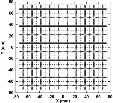
-80 -60 -40 -20 0 20 40 60 80
-80 -60 -40 -20 0 20 40 60 80
Y (mm)
X (mm)
Figure 3.2: A quasi-optical grid.
Convolution Transient Analysis
This chapter develops the equations and describes the software implemen-tation of a transient analysis based on convolution. After the introduction, section 4.2 presents the derivation of the harmonic balance (HB) equations. These are the base for the convolution transient of section 4.3. Section 4.5 presents the implementation of this circuit analysis in Transim. The nonlin-ear transmission line used to test the simulator is presented in section 4.6. Finally, the simulation results and comments are in section 4.7.
4.1
Introduction
Transient analysis of distributed microwave circuits is complicated by the in-ability of frequency independent primitives (such as resistors, inductors and capacitors) to model distributed circuits. More generally, the linear part of a microwave circuit is described in the frequency domain by network param-eters especially where numerical field analysis is used to model a spatially distributed structure. Inverse Fourier transformation of these network pa-rameters yields the impulse response of the linear circuit. This has been used in the past with convolution to achieve transient analysis of distributed circuits [16, 17, 49, 50].
The major drawback of convolution analysis has been the large time and memory requirements that result from recording and convolving the nodal voltages of the nonlinear elements. The situation worsens because of conver-gence considerations which require small time steps. This chapter develops a convolution-based transient analysis which uses state variables instead of
node voltages to capture the nonlinear response. This has two desirable ef-fects. First, the number of state variables required is less than the number of nodes of the nonlinear elements and so fewer quantities need to be recorded and convolved. Second, parameterized device models can be used as the nonlinearity is not restricted to the form of current as a nonlinear function of voltage. Parameterized device models result in stable transient analysis for larger time steps and so less discretized time history is required. Also with improved stability constant time steps can be used further improving the robustness of the convolution.
4.2
Harmonic Balance Analysis
The state variable-based convolution transient analysis presented here is based on the harmonic balance analysis as presented in [51], which in turn can be easily derived from Equations (3.7) and (3.8). Expressed in the frequency domain, the equations become
GU(f) +CΩ(f)U(f) = Sf(f) +TTIN L(X(f))
F(X(f), f) = TU(X(f), f)−VN L(X(f)) = 0
wheref is the frequency andΩis the frequency domain derivation operator. Uppercase lettes have been used to represent quantities in the frequency domain.
Ω=j2πfI,
Herej is the imaginary unit and Iis the identity matrix. It can then readily be shown that
F(X(f), f) =SSV(f) +MSV(f)iN L(X(f))−VN L(X(f), f) = 0,
where
SSV(f) =T[G+CΩ(f)]−1Sf(f) (4.1)
and
4.3
Formulation of the Convolution Transient
The system being modeled is partitioned into linear and nonlinear subnet-works1 with the linear subnetwork comprising the spatially distributednet-work characterized by EM analysis. This yields a port-based admittance matrix which is augmented by other linear circuit elements. Sources are included in the nonlinear subnetworks as they must be treated in the time domain. This implies SSV = 0. As voltages and currents at the element’s
reference nodes are not considered, the number of state variables, ns, is equal
to the number of interface ports. The frequency domain voltages at the in-terface due to the linear network is
VL(X, f) =MSVIN L(X, f) (4.3)
After doing discrete Fourier transformation the i th component of VL(f) at
the discretized time step nt, ((vL)(nt))i is
(vL(nt))i = ns
X
j=1
(vL(nt))i,j
where ((vL)(nt))i,j is defined as
(vL(nt))i,j =F−1[(MSV)i,j(IN L)j]
Here F−1 denotes the inverse fast Fourier transformation (I-FFT). For the
purposes of this transient analysis, (vL(nt))i,j must be evaluated in the
dis-crete time domain. The multiplication in the frequency domain becomes a convolution operation in the time domain. Then, the contribution of the current at the j th interface node to the voltage at the ith state variable is, assuming for now that the circuit is initially not biased (i.e., zero initial conditions),
(vL(x, nt))i,j =
(mSV(0))i,j(iN L(x, nt))j
+ Pnt−1
nτ=1(mSV(nτ))i,j (iN L(nt−nτ))j, if nt< NT
(mSV(0))i,j(0) (iN L(x, nt))j
+ PNT−1
nτ=1(mSV(nτ))i,j (iN L(nt−nτ))j, if nt≥NT
(4.4)
1The linear/nonlinear classification is not strict here since some ‘linear’ elements such