Clearing function (CF) models, which relate the expected output of a capacitated
production resource in a planning period to some measure of its workload, have shown
considerable promise for modeling workload-dependent lead times in production planning.
This fundamental workload-dependent lead time problem, also known as planning
circularity, is due to the fact that cycle time depends on the level of resource utilization in the
system, which is determined by the allocation of products to resources made by the
production planning procedure. In this thesis we focus on fitting CFs from empirical data
which is the most prevalent way to model complex stochastic systems. We use a simulation
model of a re-entrant bottleneck system as a surrogate for a real-world semiconductor wafer
fabrication environment in order to collect empirical data and compare planning models
using different CFs in terms of profit realization. We consider two CF forms: product based
CF and load based CF. We apply multiple linear regression (MLR) with three stepwise
selection procedures to product based CFs. For load based CFs, we develop simulation
optimization and heuristic algorithms to improve the initial regression fits. We implement the
load based CF form in the allocated clearing function (ACF) model and compare planning
models using product based CF to one using load based CF in extensive computational
experiments. We base our comparison on the profit realization in simulation using
non-parametric Friedman Tests. Results indicate that the MLR models including the previous
period’s variables in the regression perform better in the high utilization cases. Stepwise
© Copyright 2012 by Necip Baris Kacar
by
Necip Baris Kacar
A dissertation submitted to the Graduate Faculty of North Carolina State University
in partial fulfillment of the requirements for the degree of
Doctor of Philosophy
Industrial Engineering
Raleigh, North Carolina
2012
APPROVED BY:
_______________________________ ______________________________
Dr. Reha Uzsoy Dr. Brian Denton
Committee Chair
DEDICATION To my family
who always supported and encouraged me
BIOGRAPHY
Necip Baris Kacar, was born in 1983 in Istanbul, Turkey. He graduated from
American Robert High School in 1999 and received his Bachelor of Science degree in
Mechanical Engineering from Bogazici University, Istanbul, Turkey in 2003. Upon
graduation, he attended North Carolina State University for his Master of Science
degree in Industrial Engineering and received the degree in May 2009. He continued
his Ph.D study at the same university and started to work as a graduate industrial
trainee in SAS Institute, Cary, NC. He was elected to the Honor Society of Phi Kappa
Phi, and served as treasurer of Industrial and Systems Engineering Graduate Student
Association. His research interests include simulation based optimization algorithms
for production planning, capacity planning with Work-in-Process (WIP) using clearing
functions and supply chain management.
Upon graduation, he will join SAS Institute in Cary, NC, where he has been
working as a graduate industrial trainee for three years, as an operation research
ACKNOWLEDGMENTS
Most importantly, I would like to especially offer my gratitude to my advisor
Dr. Reha Uzsoy and appreciate his great support and excellent guidance in my
research. We have been working together for five years and all those years he went
beyond being just an advisor but offered his help in every way he can. Along with my
research, his full support in my professional career gets my deep appreciation. If I am
about to get my Ph.D. and start my professional career in the industry that I wanted,
the biggest portion of the credit goes to him. From the bottom of my heart, I truly
thank you for giving the opportunity working with you and sharing your vast
knowledge with me.
I also would like to thank my other committee members Dr. Russell E. King,
Dr. Brian Denton and Dr. James R. Wilson for serving in my committee and their
valuable comments regarding my thesis. Their feedback greatly improved my thesis
and also helped me to learn more.
I would like to recognize and thank to the entire faculty of Department of
Industrial Engineering in North Carolina State University who contributed to my
education. I already use and will be using what I learnt in this great department. I
always felt lucky to learn from the best professors that made me knowledgeable on
I also would like to recognize Hakan Sungur who works in the Department of
Industrial Engineering, for always being a great friend and helping me out with all of
my bureaucratic work. The staff in our department are very nice people, thank you
very much to all of you being friendly and helpful to me. Big thanks to all my friends
in the department making this Ph.D study much more enjoyable. I will miss our chats
in the department.
I also would like to thank my roommate Aydin Beseli who is also my close
high school friend, for making the Ph.D. life more fun and interesting.
I also would like to thank Hui Wang for being nice to me and sharing the
amazing trip memories with me across the USA.
I also would like to thank SAS Institute for supporting my Ph.D. education and
giving me the opportunity to learn their software used in this thesis, and also providing
the very valuable industrial experience.
Lastly, I would like to thank my family. I felt their support in every part of my
life. The feeling that you will make them happy and proud by achieving something in
your life was very inspiring and also a good motivation for me to work hard to write
TABLE OF CONTENTS
LIST OF TABLES ... IX
LIST OF FIGURES ... XI
CHAPTER 1. INTRODUCTION ... 1
CHAPTER 2. LITERATURE REVIEW ... 11
CHAPTER 3. SIMULATION MODEL ... 31
3.1. Simulation Model... 31
3.1.1. Simulation Parameters ... 33
3.1.2. Simulation Details ... 35
3.2. Conversion of LP Releases to Simulation Input ... 36
3.3. Data Collection for Fitting ... 39
3.3.1. Outline for Data Collection ... 40
3.3.2. Fitting Clearing Functions to Data ... 48
CHAPTER 4. EXPERIMENTAL DESIGN ... 51
4.1. Bottleneck Utilization with Different Demand Patterns: ... 51
4.1.2. Length of MTTF and MTTR ... 55
4.2. Comparison of CF Estimation Algorithms: ... 57
CHAPTER 5. CLEARING FUNCTION FITTING BY MULTIPLE LINEAR REGRESSION ... 60
5.1. Linear programming (LP) Model ... 60
5.2. Multiple Linear Regression (MLR) Models ... 64
5.3. MLR Models Experimental Results... 66
6.1. Simulation Optimization Algorithm ... 82
6.1.1. Gradient Estimation and Updating ... 83
6.1.2. SPSA Algorithm ... 86
6.2. SPSA Approaches for fitting CFs ... 89
6.2.1. SPSA ALL ... 90
6.2.2. SPSA Each ... 94
6.3. SPSA Release... 95
6.3.1. Coefficient Determination for SPSA Release ... 96
6.4. Results of SPSA Approaches ... 98
6.4.1. Iterations of SPSA Approaches ... 104
CHAPTER 7. METHODOLOGY OF SEARCH HEURISTIC ALGORITHMS ... 110
7.1. Linear Regression with Weights ... 113
7.1.1. Determination of Weights and Assignment to Observations ... 115
7.2. Search Heuristic Algorithm Results... 126
7.3. Comparison of SPSA approaches and Heuristic Algorithms ... 136
CHAPTER 8. COMPARISON OF MULTIPLE LINEAR REGRESSION FITS AND CF LOAD FITS ... 143
8.1. Comparison of MLR vs. Heuristic Algorithms... 144
8.2. Comparison of MLR vs. SPSA Approaches ... 146
CHAPTER 9. CONCLUSION... 148
9.1. Summary ... 148
LIST OF REFERENCES ... 152
LIST OF TABLES
Table 3-1: Simulation Processing Times and Batch Sizes... 33
Table 3-2: Failure Distribution Parameters... 34
Table 4-1: Failure Distribution Parameters for Long Failure ... 56
Table 5-1: Summary of Multiple Linear Regression Models ... 65
Table 5-2: The Friedman Test of Models ... 70
Table 6-1: Control Parameter Values for SPSA All ... 94
Table 6-2: Control Parameter Values for SPSA Release ... 97
Table 6-3: Cost Reduction of SPSA Approaches ... 102
Table 6-4: The Friedman Test of SPSA Approaches... 103
Table 6-5: Computational Time Performance of SPSA ... 108
Table 7-1: Cost Reduction of Search Algorithms ... 131
Table 7-2: Friedman Analysis of Search Heuristic Algorithms... 132
Table 7-3: Computational Time Performance of Heuristics ... 135
Table 7-6: Computational Effort of Best Iteration of Heuristics ... 141
Table 7-7: SPSA vs Heuristics Iteration Comparison... 141
Table 7-1: The Friedman Test of Heuristics vs. MLR ... 144
LIST OF FIGURES
Figure 1-1: Outline of Thesis ... 9
Figure 2-1: Examples of Clearing Functions Karmarkar (1989) ... 17
Figure 2-2: Classification of Optimization Problems and Solution Methodologies... 22
Figure 3-1: Re-entrant Bottleneck Model Process Chart for Products ... 32
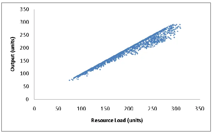
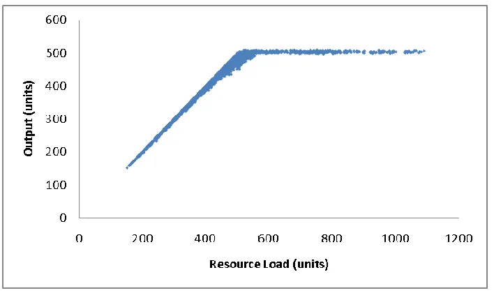
Figure 3-2: Machine 1 Output vs. Resource Load ... 42
Figure 3-3: Machine 1 Output vs. Release and Initial WIP ... 43
Figure 3-4: Machine 3 Output vs. Resource Load ... 43
Figure 3-5: Machine 3 Output vs. Release and Initial WIP ... 44
Figure 3-6: Machine 7 Output vs. Resource Load ... 44
Figure 3-7: Machine 7 Output vs. Release and Initial WIP ... 45
Figure 3-8: Machine 4 Output vs. Resource Load ... 45
Figure 3-9: Machine 4 Output vs. Release and Initial WIP ... 46
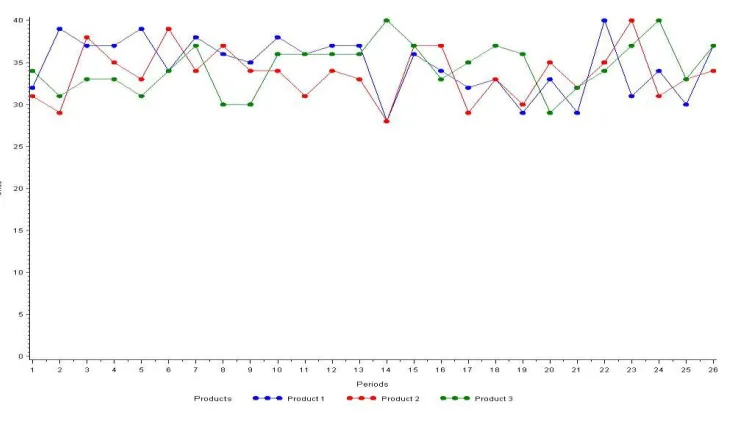
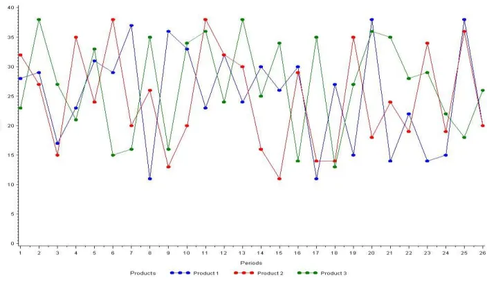
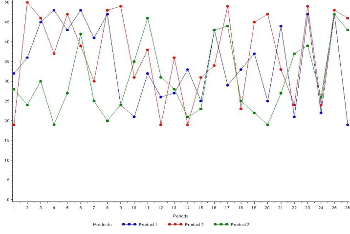
Figure 4-1: Low CV Low Utilization Demand ... 53
Figure 4-3: High CV Low Utilization Demand ... 54
Figure 4-4: High CV High Utilization Demand ... 55
Figure 4-5: Schema of Experimental Factors ... 58
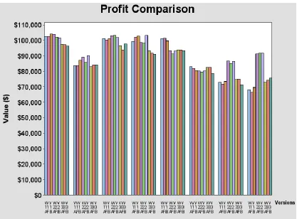
Figure 5-1: Profit Comparison of Models ... 68
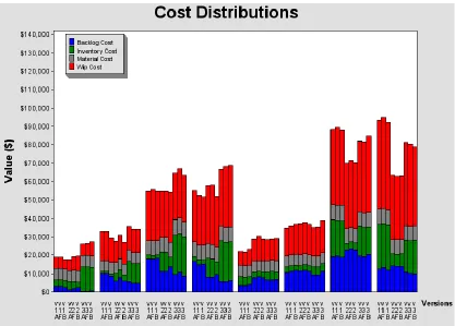
Figure 5-2: Cost Distribution of Models ... 73
Figure 5-3: Residual Plot of fitting of Machine 7 with Regression Model V2A ... 74
Figure 5-4: Normality plot of residuals ... 75
Figure 6-1: Summary of Algorithms... 82
Figure 6-2: Simulation Optimization Iterative Algorithm ... 89
Figure 6-3: SPSA Release Iteration ... 96
Figure 6-4: SPSA Approaches Profit Comparison ... 99
Figure 6-5: Cost Distribution of SPSA Approaches ... 101
Figure 6-6: Profit vs. Iteration plot for S-70-highCV case ... 105
Figure 6-7: SPSA Approach Profit vs. Iteration plot of L-90-lowCV ... 107
Figure 7-2: Assigning weights in Overestimation Case. ... 120
Figure 7-3: Profit Comparison of Search Algorithms... 128
Figure 7-4: Cost Distribution of Search Algorithms... 130
Figure 7-5: Heuristic Algorithms Profit vs. Iteration plot of S-70-highCV ... 133
Figure 7-6: Heuristic Algorithms Profit vs. Iteration plot of S-70-highCV ... 134
Figure 7-7: Cost-Tradeoff plot of all Algorithms in mean iteration time ... 139
CHAPTER 1.
INTRODUCTION
Production planning involves determining the timing and quantity of raw
material releases to the plant such that they will emerge as finished products to satisfy
customer demand on time. An executable and practical production plan must be
feasible with respect to the constraints and business rules of the production facility
while optimizing appropriate performance metrics.
Research on production planning has a long history going back to the seminal
work of Modigliani and Hohn (1955), Holt et al. (1956) and Holt et al. (1960). A
critical issue in these models is how to represent the relationship between the pattern
of work releases into the system over time and the resulting output. Understanding this
relationship lies at the heart of any production planning model, since we wish to
manage the release of raw material into the system in order to coordinate supply and
demand in an optimal manner. A critical component of this relationship is the cycle
time, the time between work being released into the system and its emergence as
finished product. We will use lead time to refer to the estimate of the cycle time used
in planning models.
In order to control the timing of releases to the plant so that the finished
product will come out on time, an estimate of cycle time is required. However, an
utilization in the system, which, in turn, is determined by the allocation of products to
resources made by the production planning procedure itself. This problem of
workload–dependent lead times in production planning is known as the planning
circularity problem (Asmundsson et al. 2009), and has been studied by many authors
(Pahl et al. 2005).
The modeling of the relationship between resource utilization and cycle time
has constituted a major challenge for the production planning field since its inception.
The problem is particularly difficult when capital-intensive plants must operate in a
highly loaded environment where they face the very complex problem of allocating
resources to products over time. It is widely recognized that the behavior of most
capacitated production resources is governed by queuing, as work arrives randomly
over time at resources whose processing capabilities are subject to varying degrees of
uncertainty. Queuing models (Hopp and Spearman 2001) have shown a nonlinear
relationship between resource utilization and cycle time. This relationship makes the
production planning task difficult, since a planning model requires knowledge of cycle
times in order to plan the production, while cycle times depend on utilization which is,
in turn, determined by the planning procedure itself. The relationship between cycle
times and utilization is nonlinear, and its effects are seen well before utilization
Most existing production planning models can be grouped under two main
headings. The first class of models considers lead time estimates as exogenous
parameters independent of resource utilization. Thus, the circularity problem is not
considered in these models. This approach is taken in the widely used Material
Requirements Planning (MRP) procedure (Vollmann et al. 2005) and most linear and
integer programming models (Johnson and Montgomery 1974), (Voss and Woodruff
2003). In MRP, the backward scheduling algorithm offsets the release of orders
backwards in time from the time that it is required to emerge as a finished product to
satisfy the demand by the value of the lead time. Since these lead times are not
updated to reflect changes in resource utilization, this approach may lead to poor
results, especially for production systems whose resource loading varies over time and
that operate at high utilization levels. In MRP, there is also an infinite capacity
assumption that may yield infeasible schedules. A number of authors such as
Billington et al. (1983) have formulated the MRP problem as a mixed integer program,
again using exogenous lead times.
Another class of exogenous lead time models are planned lead time models
(Spitter et al. 2005) where the LP formulation enables the processing of orders in
multiple periods during the lead time.
The second class of models uses either detailed scheduling algorithms or a
where the simulation model is to confirm that the release schedule suggested by the
plan is realizable in the factory and meets demand. Dauzère-Péres and Lasserre (1994)
propose a model to find a locally optimal feasible production plan.
Iterative algorithms combining LP and simulation models have been proposed
by several authors, including Kim and Kim (2001); Byrne and Bakir (1999); Byrne
and Hossain (2005); and Hung and Leachman (1996). Hung and Hou (2001) replace the
simulation model with queuing theory for lead time estimates in order to overcome time
consuming simulation runs. Essentially, these algorithms use estimates of cycle times,
corresponding to a given resource loading over time and hence a work release
schedule, and pass these estimates to an LP model as an input. The LP model in turn,
proposes a release schedule based on these cycle time estimates that form the input to
the simulation model, which is run again to estimate the new cycle times. Iteration
continues until some specified convergence criterion is satisfied. Bang and Kim
(2010) develop an iterative approach similar to that of Hung and Leachman (1996),
differing in the method of updating the parameters in the LP model after a simulation
run. They also use the observations of inventory and throughput levels from the
simulation for regrouping products into families to be used in the LP along with lead
time estimates.
These iterative simulation-LP approaches can capture the nonlinear
approach to large scale problems may not be feasible due to the time consuming
simulation runs to obtain required data. In addition, the convergence behavior of these
models is unclear and their computation time requirements may be excessive due to
the high computational burden of the detailed simulation models. Moreover, for the
models of Hung and Leachman (1996), and Kim and Kim (2001), computational
experiments have shown that assessment of their convergence can be difficult (Irdem
et al. 2008, 2010) .
Considering previous production planning models, either the nonlinear
relationship between work-in-process and output is not well captured as in the first
class of the models based on exogenous lead times, or using a simulation model to
capture this effect becomes cumbersome and intractable, together with the difficulties
in ensuring the convergence of the iterative procedure. Therefore, the effect of
capacity loading on lead times is not well incorporated into these models.
Traditional capacity planning models ignore WIP and only consider finished
goods inventory. Studies by Ettl et al. (2000) and Liu et al. (2004) for supply chain
networks that combine queuing analysis with inventory models to calculate expected
WIP and explicitly consider WIP cost in the objective function. An integer
programming model by Woodruff and Voss (2004) also includes WIP cost in the
objective function and attempts to discretize lead time estimates into brackets
computation burden is intimidating for large scale complex problems. Kekre (1984)
also considers WIP explicitly as a function of lead time in his formulation and WIP
cost in his objective function. He examines the effects of the lot sizing decision on
WIP and lead time.
Given these shortcomings of previous approaches that fail to incorporate the
effect of capacity loading on cycle times into models, the idea of clearing functions
(CFs) that represent the expected output of a resource in a planning period as a
function of the some measure of the work in process inventory (WIP) has been
proposed to capture the effects of load dependent lead times. These models have been
studied by a number of authors, including Graves (1986); Karmarkar (1989) and
Srinivasan et al. (1988). Asmundsson et al. (2006) and Asmundsson et al. (2009) have
shown promising results in several studies (Kacar et al. 2012). The advantage of these
models is that they can capture the nonlinear relationship between resource utilization
and cycle times without requiring time-consuming simulation runs as part of the
planning process. It has been shown by several authors (Missbauer 2002; Asmundsson
et al. 2006; Selçuk et al. 2007 and Asmundsson et al. 2009) that when the CF is
parameterized correctly, these models can yield superior performance over
conventional LP models. However, the use of this approach requires effective methods
of estimating the clearing functions themselves. Missbauer (2007) shows that the
clearing function depends on the work in process at the beginning of the each period,
developed clearing functions based on the combination of the Pollaczek–Khinchine
mean value formula for M|G|1 systems and Little’s Law assuming arrivals to a station are directly controlled. There are also studies by Agnew (1976) and Spearman (1991)
that develop clearing functions from queuing theory. Previous work (Asmundsson et
al. 2009) has shown that the estimation of clearing functions from empirical data,
especially with the emergence of non-stationary effects on the system, is a nontrivial
exercise for which a firm theoretical foundation still remains to be established.
Contributions of this Thesis
In this thesis, we focus on clearing function models and the estimation of CFs
from empirical data. We assume that our demand pattern is deterministic. We use a
simulation model as a surrogate for a production system to generate data from which
clearing functions can be estimated. The randomness in the system is associated with
processing times and machine failures. There are several CF forms suggested by
Graves (1986), Karmarkar (1989), and Srinivasan et al. (1988); but we focus on Load
Based CFs, where output is modeled as a function of the work in process (WIP)
available at the beginning of the period and releases in that period, i.e., Rt+Wt-1, which we refer to as load of that period (Missbauer 2002). We also examine CFs where WIP
and releases are treated as separate independent variables in regression models where
In this thesis, we aim to improve the estimation of clearing functions using a
simulation optimization approach. Generally this approach focuses on highly complex,
large scale stochastic systems that are difficult to solve analytically or model using
stochastic programming. In order to overcome this difficulty, simulation optimization
is used where the set of optimal decisions is searched using discrete event simulation
models which can include stochastic elements and complexities of a system. (Fu,
1994) provides extensive review of this area. Simulation optimization methods can be
considered under two main headings based on whether the parameter state space is
discrete or continuous. Different solution procedures are proposed depending on the
nature of the parameter state space. For discrete finite state space parameter problems,
ranking and selection and multiple comparison approaches are used which basically
utilize the statistical analysis of simulation runs. For continuous state space parameter
problems, which will be our focus, proposed approaches include response surface and
stochastic approximation techniques. Our simulation optimization approach will use
the idea of gradient estimation under stochastic approximation techniques, which also
will be explained in CHAPTER 6.
Overall, the scope and the goals of this thesis are the following;
Explore the use of several different linear regression models for
estimating clearing functions and compare the performance of the production
Obtain insight into the structure of the clearing functions and the degree
to which multiple regression can be used.
Develop a simulation optimization algorithm to identify better
performing CFs and develop heuristics to obtain good solutions in modest CPU
times if possible.
Compare different functional forms of the CFs in terms of the quality
of the resulting production plans.
Figure 1-1: Outline of Thesis
The Figure 1-1 illustrates the structure of the thesis. We present our literature
review in Chapter 2. In Chapter 3, we will introduce our simulation model and the
procedure used to obtain product based and load based CFs. In Chapter 4, we will
CF fits. In Chapter 5, we will present multiple linear regression models using product
based CF. In Chapter 6, we will introduce simulation optimization and in Chapter 7
heuristic algorithms to improve load based CF fits. In Chapter 8, we will compare our
algorithms using load based and product based CFs. We will briefly give summary
CHAPTER 2.
LITERATURE
REVIEW
There are numerous works in the literature presenting mathematical
programming models for production planning aimed at allocating capacity to multiple
products over time while satisfying demand and optimizing some performance
criterion. These algorithms include methods that consider lead time as an exogenous
parameter, and iterative methods that combine fixed lead time with simulation. The
models Johnson and Montgomery (1974), Voss and Woodruff (2003) focus on
stochastic demands are out of scope for this thesis. Recently alternative methods such
as clearing function models have been proposed, which form the main focus of this
thesis. A review of these different methods is given below, starting with the
well-known Material Requirements Planning approach.
The well-known and widely used Material Requirements Planning (MRP)
procedure discussed by Orlicky (1975) uses fixed lead time estimates that are
independent of resource utilization. A backward scheduling algorithm is used to
determine the timing of releases backwards from the due date of the product, using the
value of the lead time. The applicability and reliability of this model depend on the
accuracy of the lead time estimates, which become more unreliable in highly loaded
production environments. In addition to use of fixed lead time in MRP, there is also an
infinite capacity assumption that may yield in infeasible schedules, since it assumes
exceeds capacity. This infinite capacity assumption is addressed by the Capacitated
MRP (MRP-C) procedure developed by Tardif and Spearman (1997) which uses the
relation between WIP and cycle time, checks for WIP and capacity infeasibilities and
suggests remedies such as delaying due dates or adding capacity. This model assumes
that the lead time can be maintained as long as utilization is less than 1, i.e., the
resource capacity is not exceeded. Vollmann et al. (2005) evaluates capacity by
calculating total hours of man force needed for a given master production scheduling
(MPS) using historical data on resource allocation. This Rough Cut Capacity Planning
is a straightforward calculation to check for any obvious capacity violations. On the
other hand, Capacity Requirements Planning procedure uses more detailed
information on individual product routings and operation lead times but is still
independent of workload. Billington et al. (1983) also consider capacity explicitly in
their mixed integer programming model, including binary variables for setups. They
also suggest using minimum lead times in the formulation to represent transfer times,
not waiting times. They state that capacity and material flow constraints will implicitly
include waiting times in lead time by starting the releases in earlier periods if the
capacity constraint is tight thus products are passed through inventory.
Most LP models for production planning Johnson and Montgomery (1974);
Hackman and Leachman (1989) also use lead time estimates as an exogenous
parameter, and the accuracy of these models, especially at high utilization levels,
incorporate non integer lead times for both lag before and lag after the activity and
uneven period lengths, but lead times are still independent of workload. Spitter et al.
(2005) proposes the concept of planned lead times for supply chain operations
planning where their LP formulation enables the completion of orders before due date
while the order can be processed any time between release and due date. This model
has the flexibility that it can be processed over multiple periods compared to LP
models that assume orders released at the beginning of the period, has to be processed
in the same period.
Ettl et al. (2000) and Liu et al. (2004) develop models of supply chain
networks that calculates expected WIP from using queuing analysis. They also put
WIP cost in their objective function to find the base stock levels that minimize the cost
of meeting fill rate requirements. Kekre (1984) analyzes WIP depending on lot sizes
and comes up with an equation for WIP as a function of lot size. He states that WIP in
front of a resource depends on not individual products separately but combination of
all products WIP together. He also formulates WIP explicitly in his constraints and
includes WIP cost in the objective function.
Woodruff and Voss (2004) focus on workload dependent lead times and
piecewise linearize the nonlinear relationship between resource utilization and lead
times with the aid of binary variables that lead to mixed integer programming models
They also include a constraint to prevent a recently released order passing another that
was released earlier. This constraint also allows the model to avoid drastic changes in
releases from one period to another, thus reducing the variability in the arrivals to
stations.
To address the dependence between workload and lead times, a number of
authors have proposed iterative algorithms that combine LP models using fixed lead
times with a simulation model. Hung and Leachman (1996) propose an iterative
algorithm that estimates lead times corresponding to a given work release schedule
from simulation and passes these estimates to an LP model as an input. The LP model
in turn, determines a release schedule that forms the input to the simulation model,
which is run again to estimate the new lead times. Iteration continues until some
specified convergence criterion is satisfied. Kim and Kim (2001) propose a similar
approach where loading ratios are used as an estimate of lead times. Loading ratios
basically refer to fraction of the releases emerged as finished goods distributed to
periods. They extend the idea of Byrne and Bakir (1999) who modify only the right
hand side of the capacity constraint by multiplying the nominal capacity by the
observed utilization from simulation. Bang and Kim (2010) propose an iterative
scheme similar to Hung and Leachman where they also use discrepancies in waiting
times, WIP levels and throughput at the bottleneck between the LP solution and the
simulation output to update parameters of LP at an iteration. They also stop the
these methods is ambiguous and still not well understood Irdem et al. (2008), Irdem et
al. (2010). Due to the high computational burden of the simulation runs required to
obtain cycle time estimates, Hung and Hou (2001) replace the simulation model with
cycle time prediction models based on queuing theory and an empirical method, where
they use simulation to collect data in order to develop relationship between machine
utilization and cycle time.
Other authors have used detailed scheduling approaches in order to model
workload dependent lead times, such as Dauzère-Péres and Lasserre (1994) who
propose an iterative alternating lot sizing and scheduling problems solving procedure
to find the best possible feasible plan. They show improved performance with their
integrated approach based on experiments with several scheduling policies. Zijm and
Buitenhek (1996) apply a detailed scheduling algorithm for job shops considering WIP
in the shop and using a modified version of the shifting bottleneck method to assign
due dates to orders depending on the planned lead times.
Riaño (2003) models the lead times as independent random variables subject to
a probability distribution. In this model, expected cumulative output up to period t is equal to cumulative releases up to that period t multiplied by the corresponding probability distribution of the lead time. The requirement of this model is to satisfy the
orders with a specified probability. However this approach assumes lead time
share common resources and lead time distributions are not updated depending on the
release plan from LP.
The models described above either assume utilization independent lead times,
or requires of cumbersome simulation models to validate the feasibility of the plans
proposed by the LP models. The necessity of effective and efficient modeling of
workload dependent lead time has opened new directions in the literature. In order to
overcome these shortcomings of previous production planning models, clearing
functions provide a mechanism to relate the expected output Xt of a production resource in a planning period t to the expected work in process (WIP) level Wt over that period. The Clearing Function is similar in nature to the operating curve approach
Schoemig (1999) that describes the relation between mean cycle time and throughput,
which was developed and used to predict the performance of the manufacturing line.
They also show the degrading effect of variability caused by machine down times.
Several examples of clearing functions in the literature are depicted in Figure
2-1. The “Constant level” function places a fixed upper bound on production. It does
not have any lead time constraint and assumes instantaneous production no matter
what the WIP level is. Graves (1986) proposes a clearing function in the form of
Xt = α Wt, where output Xt at time t is considered a linear function of WIP. This “constant proportion” function assumes a fixed lead time of 1/α can be maintained at
operated in the range that this fixed lead time assumption will hold. This function may
yield infeasible levels of output at high WIP levels, and so needs to be limited by a
fixed capacity which is shown as the “combined” clearing function. Karmarkar (1989)
proposes a linear clearing function where output increases as a concave
non-decreasing function of Wt, reaching an asymptotic maximum. Srinivasan et al. (1988) propose another clearing function which is a concave, non-decreasing function of
WIP. Figure 2-1 shows these types of functions as the “effective” clearing function.
Figure 2-1: Examples of Clearing Functions Karmarkar (1989)
Missbauer (2002) discusses the limitations of clearing function models such as
the fact that they limit the output by a function of the expected total load and the
distribution of the arrival period of the work expected to contribute to the load in
determines the amount of work released in each planning period and can handle
different load patterns without requiring additional load balancing parameters. Early
clearing function models had difficulty in modeling the behavior of multiple products
since when products compete for capacity, then one product may end up waiting
indefinitely while other products are processed in very short lead times. In order to
solve this problem, Asmundsson et al. (2009) propose an allocated clearing function
formulation for multiple products where capacity is allocated to individual products.
This model forms the basis for our work in this thesis, and will be described in more
detail in CHAPTER 6.
Clearing functions can be derived analytically using steady-state or transient
queuing models, or estimated empirically from empirical data. Different authors have
implemented somewhat different approaches. Agnew (1976) proposes a throughput
function where service rate is a function of the number in queue and suggests using it
in optimal control policy context. Spearman (1991) derives a clearing function using
closed queuing networks, conjecturing a relation between mean cycle time and WIP,
and taking one observation from simulation to specify congestion of the system.
Asmundsson et al. (2009) formulate the clearing function as a relationship between the
expected throughput of a resource in a planning period as a function of the
time-average WIP level at the resource during the period from empirical data. Other
authors, such as Karmarkar (1989) and Missbauer (2002) assume the clearing function
process available at the start of the period and the material released during the period.
Zäpfel and Missbauer (1993a) use a simulation model to estimate Clearing Functions
based on the expected workload, and observe discrepancies between planned and
actual WIP in simulation. Missbauer (2009) shows that the clearing function depends
on the work in process at the beginning of the each period due to transition behavior of
the system within the planning period and corrects the Clearing Function to minimize
the discrepancy between transient and non-transient Clearing Function. Selçuk et al.
(2007) have derived transient clearing functions analytically using Pollaczek–
Khinchine mean value formula and Little’s Law.
In this thesis, we focus on empirical estimation of Clearing Functions from
simulation data, which has been the most prevalent approach in the literature
especially for complex production systems. In this approach, the production system
under study is simulated and data collected from the simulation model in each
planning period on the quantities of interest, which depend on the independent
variables postulated for the clearing function. Once the data have been obtained, they
are fit empirically using some form of regression analysis to a predefined functional
form.
In the literature there are two typical functional forms that are suggested to
estimate the clearing functions. Karmarkar (1989) proposes the form ( ) ;
K1 represents the maximum possible output in a period and K2 defines the curvature of the clearing function. These two forms are types of “effective” clearing functions as
shown in Figure 2-1. Asmundsson et al. (2009) use the CF form suggested by
Srinivasan et al. (1988) to fit CF from simulation data and observe the non-stationary
behavior discussed by Missbauer (2009). They modify the CF by fitting a curve that
lies below a certain percentage of the data points to minimize the overestimation.
In our research, we consider two different measures of workload. We first
consider the WIP and Release of resource k in period t separately, yielding
( ) and relate them to output using multiple linear regression.
Next, we consider W in terms of the sum of the releases within a period and initial WIP levels ( ), instead of the time averaged WIP that has been
studied in previous research.
In our research, we take a different approach from the literature by estimating a
clearing function for each individual product based on the release quantities and WIP
levels of this product and those of other products in the current and immediately
preceding periods. The values of the state variables of interest are regressed against
the output of each product. In this way we hope to obtain insight into which variables
are important to include in the clearing functions and which can safely be omitted. In
the second part, we introduce load based fitting which considers the sum of releases in
output, and suggest a simulation optimization approach and search heuristic
algorithms to improve our fit. This will essentially be an extension of the Asmundsson
et al. (2009) approach of using a percentile level of the data to fit the CF, where the
parameters are determined by simulation optimization.
In this thesis, both our simulation optimization approach and search heuristics
for improved Clearing Functions will focus on the load based form where output is a
function of the sum of planned input in period t and WIP available at the beginning of period t for machine k given by
( ) ( 2.1)
We develop CF improvement algorithms that are based on an optimization via
simulation approach. (Fu, 1994) has an extensive review paper on this area, discussing
several methods. This area has attracted attention due to increased efforts in
optimization of stochastic discrete event systems where simulation is used to estimate
the performance of system to overcome the computational and inherent complexities
of the system. Simulation optimization is an approach in which the space of decision
variables is searched to obtain the best performance estimate from simulation. The
optimization problem is considered under two categories: discreet and continuous state
space. Here, the state space is the collection of the parameters or decision variables in
performance estimates in simulation. The classification and solution methodologies
are given in Figure 2-2. The general problem setting of these problems is,
( ),
where ( ) ( ) is the performance measure of interest; ( )the sample
performance, with denoting the vector of simulation replications and the vector of
controllable parameters or decision variables. is the set of all possible selections of
. The optimum value of ( ) can be defined as finding that will yield
( ). In these problems, our controllable parameter set can be discrete
or continuous.
Figure 2-2: Classification of Optimization Problems and Solution Methodologies
We now present solution methodologies for discrete state space problems
where the nature of the parameter state space is discrete. Depending on the problem,
parameter set is finite. Even though the parameter set is infinite, reduction or
approximation techniques can be used to reduce the problem state space to a finite set.
Under this category, there are two major solution methodologies; Ranking and
Selection and Multiple Comparisons. For the Ranking and Selection, in general there
are two approaches in literature: Indifference Zone and Subset Selection. The former
approach uses a specified probability value p that, with the selected vector of
parameters , { ( ) ( ) } where denotes the so called
“ indifference zone” i.e., with the selected vector , ( ) is within of the optimal
value ( ) with probability p. In the Subset Selection approach, the aim is to choose a subset of at most m such that one of the selected will guarantee the probability relation stated above. These two approaches can be used to complement
each other in a problem with a large set of possible selections such that Subset
Selection can be used to reduce the number of sets and then the Indifference Zone
approach can be used to find the among the reduced set that will be different from
the optimum within a specified indifference zone . For the other methodology used
for discrete finite space problems, Multiple Comparisons, the basic idea is to do all
pairwise comparisons of performance of all and interpret the difference in terms
of confidence intervals to choose the best performing parameter vector . The
comparisons tests may contain paired t tests or multiple comparisons tests such as
using Bonferroni inequality to account for multiple comparisons applied
We now discuss continuous state space problems where the parameters are
continuous. We start with Response Surface Methodology, where a polynomial
function of appropriate degree is fit to the response (performance measure of interest)
of the system. There are two phases. In the first phase, a least-squares regression is
applied to the initial experimental runs and a new subregion is chosen to be explored
through the equation where is nth explored subregion , is the estimate of the gradient from the fitted linear response obtained in the first phase
and is the step size. This is repeated until gradient gets close to zero that no more
regions to be explored are obtained. In the second phase, a quadratic response surface
is fitted to the response using more detailed experimental runs and an optimum is
obtained analytically from this fit. There is a shift of focus in this methodology in that
the main interest becomes finding an improved response over the current conditions
than finding the optimum one.
Next, we present the Stochastic Approximation method for continuous state
space that our simulation optimization approach will use for estimating gradients. This
algorithm begins with best guesses of optimal parameter values which are updated
iteratively based on the estimate of the gradient of the performance metric with respect
to the parameter. The Response Surface methodology also implements a gradient
based algorithm whereas the gradient estimation is obtained from regression model.
( ) in the original problem setting; however there are problems of local
optimality or slow rate of convergence.
The general form of the Stochastic Approximation algorithm is as follows:
Compute ( ) where is the parameter set at the n’th iteration,
is the step size, is the estimate of ( ) and is a projection onto which if
goes out of feasible region, returns to the feasible region; one such is
assigning to the previous iteration vector . In this setting, some of the main
questions are, what should the step size be and how should be calculated. For
step size, in practice, decreasing the step size when the gradient changes direction has
been shown to perform better compared to harmonic series of step sizes ⁄ that in
practice shows slower convergence. For gradient estimation, in general there are four
techniques: finite differences, likelihood ratio, perturbation analysis and frequency
domain experimentation. The way to estimate the gradient with the finite difference
technique is to run multiple simulations to obtain an approximation of the gradient.
One version of finite differences is
̂ ̂ ̂ where p denotes the number of elements in the parameter set.
̂ ̂( ) ̂( )
’s are the difference parameters whose values represent a tradeoff between too much
noise (using small values) and too much bias (using large values). In order to have
convergence the ’s should approach zero. This gradient estimation technique is most
generally applicable but shows slower convergence due to the computational
intensiveness of the technique. In this symmetric finite difference technique, 2p
simulation runs are required for gradient estimation. In order to overcome the
potentially long CPU time caused by many simulation runs, Spall (1998) suggests the
Simultaneous Perturbation Stochastic Approximation (SPSA) technique which
requires two simulation runs for estimating the gradient. The gradient estimation takes
the form
̂ ̂( ) ̂( )
̂ ̂
Here is a p-dimensional random perturbation vector such that each component of is independently generated from a zero mean distribution. A simple
choice of this type would be ±1 Bernoulli distribution with probability of 0.5 for each
outcome ±1. The gradient estimation ̂ reflects the simultaneous perturbations of all
components of in contrast to component by component perturbations in finite
difference gradient estimation. Updating is same as in other stochastic
are obtained by choosing nonnegative coefficients for a, c, A. α and γ and then at each
iteration and are calculated with the equations = ( )⁄ and ⁄
,respectively. Iteration is terminated if there is little change in several successive
iterates or a specified maximum number of iterations is reached.
Perturbation Analysis estimates gradient by applying a what if analysis,
computing what would happen if , which is the nominal case, had been
where is infinitesimally small. One of the main assumptions in this technique is
that this small change in parameter will not alter the order in which the events happen
in the system. Basically this technique takes the partial derivatives of the performance
metric of system with respect to the parameters and estimates the gradient in this way.
The Likelihood Ratio technique uses the idea of differentiating the underlying
probability of the system and requires the differentiation property of the probability
measure. Expectation of performance measure is expressed as,
( ) ∫ ( ) ( ) where ( ) is the cumulative distribution function of
random vector X depending on parameter vector . Differentiating the previous
equation yields, ( ) ( ) ( ( ) so in a single simulation run, estimates of
the derivative of performance measure and the performance measure itself can be
obtained. The last technique that we present for gradient estimate is Frequency
according to sinusoidal function during simulation. The parameter vector is stated as
( ) ( )
where is vector of oscillation amplitudes and w the vector of oscillation frequencies. The gradient estimation problem becomes that of estimating the gradient at
( ) which is ( ) It is achieved by approximating J around using a second order Taylor expansion and taking the partial derivatives respect to the
parameter vector.
We plan to use a simulation optimization approach, specifically the
Simultaneous Perturbations Stochastic Approximation (SPSA) technique, for
optimizing our clearing function fitting parameters as explained in Section 3.3. The
choice of technique is based on the fact that it requires only 2 simulation runs for
gradient estimation at each iteration, compared to 2p simulation runs for the Symmetric Finite Difference method. The ease of implementation is also an advantage
for SPSA. In our setting, our decision variables for the simulation optimization
problem are the Clearing Function constraint parameters of each machine: intercept
and slope values of each linear segment used to approximate the clearing function.
These decision variables are continuous. Formally the general scheme of the SPSA
Definitions:
k : index of Machines;
: Decision variables
: Decision variables space,
( ) : Profit Realization at Simulation of replication with
( ) : Expected Profit Realization with ; ( ) ( )
Objective function:
( );
Gradient Estimation using SPSA technique at iteration n:
[ ̂ ̂]
̂ ̂( ) ̂( )
Updating Decision Variables:
is the gain at iteration n.
Algorithm:
Step 1: Run Simulation with and obtain ( )
Step 2: Calculate ̂
Step 3: Update
Step 4: if ( ( ) ( )) stop and report ( ); is small number
Else n=n+1, and return to Step 1..
In our research, we will also develop a heuristic algorithm that benefits from
the idea of gradient estimation but with a different approach which uses the dual
solutions of the LP model for gradient estimates. This approach will be explained in
detail in CHAPTER 7. The motivation for the heuristic algorithm is to avoid potential
time consuming calculations for gradient estimation due to the simulation runs
necessary at each iteration and also the potential large number of iterations for the
algorithm to converge.
In this thesis, we will provide the performance comparison of these two
different CF fitting approaches and present their results. In the next section we present
the simulation model of the testbed factory that will be the source of the empirical data
CHAPTER 3.
SIMULATION
MODEL
Our data collection of variables of interest for estimation of clearing functions,
comparison of performance for our fitted CFs and our algorithms (simulation
optimization, search heuristic algorithms) will use a simulation model as a surrogate
for the real factory. This model, originally developed by Kayton et al. (1997) will
provide the empirical data on output and WIP used to fit the clearing functions, and to
assess the performance of the resulting clearing functions by simulating the execution
of the production plans obtained using them. Therefore, in the following sections, we
present the details of the simulation model, steps to convert LP releases to simulation
input, and the data collection procedure used in fitting the CF.
3.1. Simulation Model
Our simulation model of a re-entrant bottleneck system was built with the
attributes of a real-world fab environment, studied in previous research (Kayton et al.
1997). The major characteristics of wafer fabrication, including a re-entrant bottleneck
process, unreliable machines, batching machines, and multiple products with varying
process routings and number of operations are included in the model. Wafers move
through the facility in lots of a standard size. There is a distinct re-entrant bottleneck
machine representing the photolithography process. The processing times for all other
has a utilization approaching that of the bottleneck. The model has batching stations
(Stations 1 and 2) early in the process, representing the furnaces which perform the
diffusion and oxidation processes, where up to four lots can be processed
simultaneously. The remaining stations process one lot at a time.
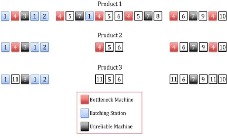
Figure 3-1: Re-entrant Bottleneck Model Process Chart for Products
There are 11 machines (stations) and 3 products in this model. The number of
operations for Products 1, 2 and 3 are 22, 14 and 14, respectively. Station 4 is the
re-entrant bottleneck machine shown in red in Figure 3-1. There are two servers at
Station 4. Products 1 and 2 visit the bottleneck station 6 and 4 times, respectively.
Product 3 does not use the bottleneck machine. This product visits Station 11, which is
the bottleneck utilization. There are two batching machines, machines 1 and 2, shown
in blue in Figure 3-1, where up to four lots can be processed simultaneously as a
batch. The minimum batch size required is two lots. The batching stations can run lots
of different product types in the same batch. There are two unreliable machines,
machines 3 and 7, shown in black in Figure 3-1, which are subject to considerably
longer failures than the other stations and can cause starvation at the bottleneck
station.
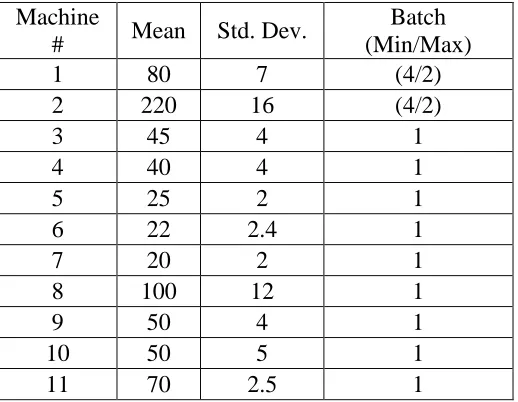
3.1.1. Simulation Parameters
The distributions of processing times and failures and their parameters will be
presented in this section.
3.1.1.1. Simulation Processing Times
Table 3-1: Simulation Processing Times and Batch Sizes
Machine
# Mean Std. Dev.
Batch (Min/Max)
1 80 7 (4/2)
2 220 16 (4/2)
3 45 4 1
4 40 4 1
5 25 2 1
6 22 2.4 1
7 20 2 1
8 100 12 1
9 50 4 1
10 50 5 1
The processing times for all stations are summarized in Table 3-1. All
processing times follow a lognormal distribution, and are given in minutes. The
standard deviations of process times are within 10 percent of the mean. The processing
times for all operations on a given machine, regardless of product type, are assumed to
follow the same distribution. This is clearly an approximation of the real situation in
practice, but was validated by management during the original study by Kayton et al.
(1997) as a reasonable starting point.
3.1.1.2. Failure Distribution Parameters
Table 3-2: Failure Distribution Parameters
MTTF MTTR
Machine
# Alpha Beta Mean
Std.
Dev. Alpha Beta Mean
Std. Dev.
3 7200 1 7200 84.9 1200 1.5 1800 52.0
7 7200 1 7200 84.9 1200 1.5 1800 52.0
The mean time to failure (MTTF) and mean time to repair (MTTR)
distributions follow gamma distributions with parameters given in Table 3-2.
Machines 3 and 7 are unreliable machines that can produce a product in a very short
time but can starve the bottleneck due to poor availability. The mean and standard
deviation values are calculated using the formulas for gamma distribution as follow:
The values are in minutes. Availability can be calculated as follows:
(3.1)
This can be interpreted as on average machines are operating 80% of the time.
In the simulation model, the failures are implemented as preemptive. We will
experiment with different levels of variability in down and repair time in our
experiments, while holding the average availability constant.
3.1.2. Simulation Details
The simulation model is created in Simulation Studio 1.6 (SAS)
(www.sas.com) that runs on a Intel PC with a Intel(R) Pentium D CPU 3.40 GHz
processor and 2GB of RAM, under Microsoft Windows XP Professional.
The period length for the production planning models is 7 days. Our planning
horizon is 26 periods, thus simulation is run for 26 periods. An LP solution provides
noninteger release quantities that need to be converted into whole quantities. The
transfer of release inputs from LP to simulation will be discussed in Section 3.2. The
release entities are created at the beginning of each day by reading the data from the
converted releases to whole numbers. After presenting our simulation model, we will
discuss the conversion of LP releases to simulation input and data collection in the
3.2. Conversion of LP Releases to Simulation Input
The release schedule that is found by LP models specifies the number of lots of
each product to be released in each planning period, and may be fractional. Simulation
requires an integer number of lots, so in order to give the release schedule suggested
by LP as an input to simulation, the fractional values need to be rounded to integer
values.
In addition to being fractional, the release quantities suggested by the LPs are
weekly quantities. In our simulations, we assume that the planned releases for a
planning period are uniformly distributed over that period. Hence we convert the
weekly release schedules to daily release schedules for that period.
In order to address these issues, we use an algorithm that rounds some release
values up and some values down. We do not simply round up all values since the
cumulative effect could lead to significant excess production. In our algorithm, we
first divide the planned release quantity for each period, which is one week in our
study, into equal daily release quantities by dividing the weekly release quantity by
seven for all periods. The release quantity of the first day of that period is always
rounded up to its nearest integer value, and the difference between the planned
fractional releases and obtained integer releases is recorded. If the cumulative
difference is greater than 0.001, the next value is rounded down to its nearest integer,
cumulative release schedule of the planning horizon from LP and cumulative adjusted
release schedule for simulation input close to zero. Thus the planned LP release
schedules and simulation input schedules are matched closely, enabling us to compare
LP outputs to simulation outputs more accurately. The steps of this algorithm can be
summarized as follows.
Step 1: Divide the weekly schedule into equal daily schedules by dividing the
release schedule from LP by seven.
Step 2: Round up the first release day of that period.
Step 3: Check whether cumulative differences of actual releases from LP and
obtained integer releases are greater than 0.001 or not. If the quantity is greater, round
down the corresponding fractional release. If it is less than 0.001, than round up the
corresponding fractional release. Go to the next daily schedule.
Step 4: When the calculations are done for one weekly schedule, start over the
process with the next weekly schedule, following Steps 1, 2 and 3.
The steps are summarized as a pseudocode below. The value of Rounded( )
corresponds to obtained integer value of using the operations explained in the
previous paragraph.
Step 1: Rdaily=Rweekly/7
Step 2: RoundUP(R1t)
Step 3: do d=2 to 7; d is number of the day of the week.
if (∑ ∑ ( ))
Then RoundDown( );
Else RoundUP( );
End;
Step 4: Set t=t+1 until t=T. Continue with steps 1-4.
Using the steps above, we obtain whole numbers for release lots of each day
that gets into the simulation. After the lots are released into the system before their
first operation, the products are sequenced in the order of products 1, 2 and 3
repeatedly. The excess amounts of products are put in front of other products
following the same sequencing logic. For example, we have 4 lots of product 1, 3 lots
of product 2, and 2 lots of product 3, then the sequencing of lots will be
1-1-2-1-2-3-1-2-3. This sequence will processed in the station in the order from left to right, product
type 1 being first to be processed. We use this procedure to obtain more uniform
output rates among products. Lots are dispatched in First-in-First-Out order on all
In the next section we discuss how the data is collected from the simulation
model to use in fitting the clearing functions.
3.3. Data Collection for Fitting
In this study, we investigate two forms of clearing function where in the first
form output is a function of releases within the period and WIP at the beginning of the
period considered separately whereas in the second form output is a function of sum of
release and WIP. These functional forms are given below.
( ) (3.2)
( ). (3.3)
For these CF functional forms, the data required in fitting is different. For the
load based functional form, ( ), CFs are fit based on each
machine, not individual products, where Xkt represents the total output of machine k in period t. Note that in our simplified model, all operations at a machine have the same processing time distribution, regardless of product type or operation, thus variables are
in units of quantities. The quantity Wk,t-1 represents the total number of lots available in WIP at the beginning of the period at machine k and Rkt the total number of lots
released to machine k in period t. The product based functional form
index. Thus CFs are based on product type in addition to which machine they are
processed on.
In summary, the data needed to fit a function of form
( ) for each machine k are the total releases within a period Rkt,, total number of WIP at the beginning of the period Wk,t-1 and total output in that period Xkt. For the functional form ( ), we need the individual
quantities of each product mentioned above. Denoting g as the product index, note that ∑ , ∑ and ∑ .
3.3.1. Outline for Data Collection
Our focus in this thesis is to fit CFs from empirical data. We use our
simulation model to obtain our data. In order to obtain data that has basic coverage of
several WIP Wkg,t-1 and Release Rkgt scenario combinations and corresponding outputs Xkgt, we experiment with several long simulation runs corresponding to different bottleneck utilization levels. The reason for having runs with several bottleneck
utilizations is to observe many different combinations of Wk,g,t-1 and Rkgt so as to obtain CFs that better reflect the characteristics of the resources over a wide range of
operating conditions. We follow the steps below to obtain data to fit our clearing
function. Here, we note that, the release plans used in these long simulation runs are
created randomly with the aid of the normal distribution and executed in the