Heuristic assignment of CPDs for probabilistic inference in junction trees

(1)

University of Windsor University of Windsor

Scholarship at UWindsor

Electronic Theses and Dissertations Theses, Dissertations, and Major Papers

2009

Heuristic assignment of CPDs for probabilistic inference in

junction trees

Mirza Tania Nasreen University of Windsor

Follow this and additional works at: https://scholar.uwindsor.ca/etd

Recommended Citation Recommended Citation

Nasreen, Mirza Tania, "Heuristic assignment of CPDs for probabilistic inference in junction trees" (2009). Electronic Theses and Dissertations. 7900.

https://scholar.uwindsor.ca/etd/7900

(2)

Heuristic Assignment of CPDs for Probabilistic Inference in

Junction Trees

By

Mirza Tania Nasreen

A Thesis

Submitted to the Faculty of Graduate Studies

Through Computer Science

In Partial Fulfillment of the Requirements for

The Degree of Master of Science at the

University of Windsor.

Windsor, Ontario, Canada

2009

(3)

**1*1**

Library and Archives Canada

Published Heritage Branch

395 Wellington Street OttawaONK1A0N4 Canada

Bibliotheque et Archives Canada

Direction du

Patrimoine de I'edition

395, rue Wellington OttawaONK1A0N4 Canada

Vour file Votre reference ISBN: 978-0-494-57625-0 Our file Notre r6f6rence ISBN: 978-0-494-57625-0

NOTICE: AVIS:

The author has granted a

non-exclusive license allowing Library and Archives Canada to reproduce, publish, archive, preserve, conserve, communicate to the public by

telecommunication or on the Internet, loan, distribute and sell theses

worldwide, for commercial or non-commercial purposes, in microform, paper, electronic and/or any other formats.

L'auteur a accorde une licence non exclusive permettant a la Bibliotheque et Archives Canada de reproduire, publier, archiver, sauvegarder, conserver, transmettre au public par telecommunication ou par I'lnternet, preter, distribuer et vendre des theses partout dans le monde, a des fins commerciales ou autres, sur support microforme, papier, electronique et/ou autres formats.

The author retains copyright ownership and moral rights in this thesis. Neither the thesis nor substantial extracts from it may be printed or otherwise reproduced without the author's permission.

L'auteur conserve la propriete du droit d'auteur et des droits moraux qui protege cette these. Ni la these ni des extraits substantiels de celle-ci ne doivent etre imprimes ou autrement

reproduits sans son autorisation.

In compliance with the Canadian Privacy Act some supporting forms may have been removed from this thesis.

Conformement a la lot canadienne sur la protection de la vie privee, quelques

formulaires secondaires ont ete enleves de cette these.

While these forms may be included in the document page count, their removal does not represent any loss of content from the thesis.

Bien que ces formulaires aient inclus dans la pagination, il n'y aura aucun contenu manquant.

(4)

AUTHOR'S DECLARATION OF ORIGINALITY

I hereby certify that I am the sole author of this thesis and that no part of this

thesis has been published or submitted for publication.

I certify that, to the best of my knowledge, my thesis does not infringe upon

anyone's copyright nor violate any proprietary rights and that any ideas, techniques,

quotations, or any other material from the work of other people included in my thesis,

published or otherwise, are fully acknowledged in accordance with the standard

referencing practices. Furthermore, to the extent that I have included copyrighted

material that surpasses the bounds of fair dealing within the meaning of the Canada

Copyright Act, 1 certify that I have obtained a written permission from the copyright

owner(s) to include such material(s) in my thesis and have included copies of such

copyright clearances to my appendix.

I declare that this is a true copy of my thesis, including any final revisions, as

approved by my thesis committee and the Graduate Studies office, and that this thesis has

(5)

ABSTRACT

Many researches have been done for efficient computation of probabilistic queries posed

to Bayesian networks (BN). One of the popular architectures for exact inference on BNs

is the Junction Tree (JT) based architecture. Among all the different architectures

developed, HUG1N is the most efficient JT-based architecture. The Global Propagation

(GP) method used in the HUGIN architecture is arguably one of the best methods for

probabilistic inference in BNs. Before the propagation, initialization is done to obtain the

potential for each cluster in the JT. Then with the GP method, each cluster potential

becomes cluster marginal through passing messages with its neighboring clusters.

Improvements have been proposed by many researchers to make this message

propagation more efficient. Still the GP method can be very slow for dense networks. As

BNs are applied to larger, more complex, and realistic applications, developing more

efficient inference algorithm has become increasingly important. Towards this goal, in

this paper, we present some heuristics for initialization that avoids unnecessary message

passing among clusters of the JT and therefore it improves the performance of the

architecture by passing lesser messages.

Keywords: Artificial intelligence, Bayesian network, Probabilistic inference, Junction

(6)

DEDICATION

This thesis is dedicated to my parents who have supported me all the way since

the beginning of my student life.

This thesis is dedicated to the people of my country Bangladesh who have always

dreamt to get a foreign degree but couldn't make it because of not having enough

financial support.

Also, this thesis is dedicated to my husband Muhammad N Hasan who has been a

great source of motivation and inspiration.

Finally, this thesis is dedicated to all my friends who were always there when I

(7)

ACKNOWLEDGEMENTS

1 would like to give my sincere gratitude to my supervisor Dr. Dan Wu, for his

excellent supervision, guidance, and encouragement through out this research work.

Without his help and his great patience to me, this work presented here would not have

been possible.

I would also like to thank my internal reader, Dr. Robin Gras and my external

reader, Dr. Xiang Chen for participation as my thesis committee and spending their

precious time to review this thesis and putting down their comments, suggestions on the

thesis work. Their confidence in my abilities has been unwavering, and has helped to

make this thesis a solid work.

I would like to acknowledge my husband Muhammad N Hasan for his patience,

love, support and encouragement. His wisdom and guidance helped me solve many

difficult problems during my research.

Finally, I am very grateful to all my family and friends for being supportive and

(8)

LIST OF TABLES

TABLE 4-1 TOTAL NUMBER OF ARITHMETIC OPERATIONS REQUIRED BY HUGIN 42

TABLE 4-2 MULTIPLE ASSIGNMENTS OPTIONS FOR NODE a AND e 46 TABLE 4-3 SUMMERY OF THE MOTIVATION EXAMPLE PRESENTED IN SECTION 4.2 52

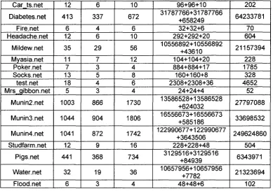
TABLE 4-4 INDEXING OF CLUSTERS BASED ON THEIR NUMBER OF NODES 64 TABLE 5-1 FREQUENCY OF THE OCCURRENCE OF THE MULTIPLE ASSIGNMENT OPTIONS FOR

A C P D 70 TABLE 5-2 COMPARISON OF THE PERFORMANCE IN TERMS OF NUMBERS OF MESSAGES

PASS 72 TABLE 5-3 COMPARISON OF THE PERFORMANCE IN TERMS OF NUMBERS OF OPERATIONS. 74

(12)

1. INTRODUCTION

Most of the real-world problem domains are almost always incomplete because not all

the relevant variables and relationships are known. For this reason the models that most

accurately reflect available knowledge are often probabilistic. In the early days of

rule-based programming, the most common methods used variants on probability calculus to

combine certainty factors associated with applicable rules [Go 1961], [HM1989],

[Chi 991]. Although it was recognized that certainty factors did not conform to the

well-established theory of probability and also the probabilistic techniques available at that

time required specifying either an intractable number of parameters, or an unrealistic set

of independence relationships, these probabilistic techniques were nevertheless favored.

Thus real-world domains quite naturally lead to partial dependency graph models that are

probabilistic [Chrl998], [SDLC1993].

'Graphical modeling language for representing uncertain relationships' is the

"breakthrough" for which methods firmly based on probability theory have begun to gain

acceptance in the computer-science and uncertain-reasoning communities. The graphical

representation of probabilistic relationships among events has been the subject of

considerable research [KJ1999], [Je2001]. A primary advantage of using a graphical

representation of probabilistic relationships is the efficiency that results. Belief updating

in dependence graphs has been studied in an axiomatic way within the frame of local

computation in graphical structures, developed by Shafer and Shenoy [SSI988],

[SSI990]. A particular type of probabilistic graphical representation, called Bayesian

Networks (BN) [Pel986a], which is by far one of the most popular probabilistic graphical

models. This knowledge representation has been termed differently in the literature. In

addition to being called bayes-belief net [Pel986a]; they have been termed causal nets

[Go 1961], [Go 1983], causal network [LSI988], probabilistic cause-effect models

[Rol968], probabilistic causal networks [Col984], and influence diagrams [Shal986],

(13)

Bayesian Networks (BNs) are currently the dominant uncertainty knowledge

representation and reasoning frame work in artificial intelligence (AI) [GH02]. Many

methodologies have been proposed as the solution for reasoning with uncertainty,

including certainty factor, fuzzy sets, dempster-shafer theory, and probability theory. The

probabilistic approach of Bayesian network is now by far the most popular among all

those alternatives, mainly due to a knowledge representation framework. The success of

BNs relies on its capability of acquiring and representing conditional independency. The

representation rigorously describes these relationships, yet includes a human-oriented

qualitative structure that facilitates communication between a user and a system

incorporating the probabilistic model.

Probabilistic inference with BN is the task of computing the posterior probability

distribution of each value of a node in BNs when values of other variables are known. A

typical application of probabilistic inference involves constructing a probabilistic model,

such as a BN, and then applying algorithms to the model to compute answers to

probabilistic queries. Probabilistic queries are answers that are augmented with

probabilistic estimates of the validity of the answers. Probabilistic answers to queries

over uncertain data have been well studied in the literature [BH1986], [ChG1989].

[Col990]. There are two kinds of probabilistic inference presented in the literature.

'Exact inference' means computing the exact posterior probability distribution and

'Approximate inference' produces an inexact, but within small distance of the correct

answer. Many researches have been done for efficient computation of exact probabilistic

queries posed to BNs [LiD1994], [ZP1994], [Nel990], [Ne2003]. One of the well known

techniques for exact inference for multiply connected BNs is clustering [ZY1998],

[Le2000]. Among many inference algorithms, the most popular and commonly used

exact BN inference algorithm is the Jensen's version [JLO1990] of the Lauritzen and

Spiegelhalter's clique-tree propagation algorithm [LSI988]. In this algorithm, a BN is

first converted into a secondary structure (called join tree or junction tree) and

computations are done on that junction tree (JT) for probabilistic inference. The key step

(14)

of the JT. There are two main architectures for propagating messages in a JT: the

Shenoy-Shafer architecture [SS1986] and the HUGIN [JLO1990], [AOJJ1989] architecture.

Among all the well known architectures implementing the idea for propagating

messages on JT, HUGIN architecture is probably one of the most efficient architectures

in the field of uncertain reasoning [ParDar2003], [SalJ1997]. This architecture allows

propagation of messages through the clusters of the JT. This message propagation is

termed as the global propagation (GP) method by many researchers [SAS1994] [Hdar96],

as this architecture performs probabilistic inference by propagating local information but

maintaining the global properties (i.e. probability density over all the variables) of the

original BN. Among various algorithms developed, the GP method used in the HUGIN

architecture for performing message passing is well received and implemented [LSI988],

[JLO1990], [LeShl998]. This propagation method of HUGIN works efficiently in terms

of inference under uncertainty, but its performance degrades quickly for dense networks

[PPGH1994]. Its complexity is exponential in the size of the largest cluster of the

junction tree [Dar2003]. Thus, computationally exact inference can be extremely

expensive.

HUGIN architecture consists of four sequential steps: (1) transforming the BN

into JT, (2) initialization on the JT, (3) propagating potentials on the JT, and (4)

answering queries. Efficiency of the HUGIN architecture largely depends on the GP

method [ParDar2003], [Dar2003]. In order to improve the efficiency of the HUGIN

architecture, many modifications on the HUGIN architecture have been done by

researchers [Dawl992], [SchS1998], [ParDar2003], [BZKPC2006]. All those existing

modifications for faster inference mostly focus on the efficiency of the propagation

phase. And in those works the initialization phase follows the same classical approach

used in the HUGIN architecture. As the initialization is concerned with the formation of

cluster potentials which are the main participants later in GP, this phase has a potentially

significant impact on the subsequent propagation phase which consists of a lot of

message passing. Thus, the improvement of the initialization can possibly also improve

(15)

Recently, by utilizing the semantic meaning of message propagation, Wu and Jin

[WuJ2006] were able to propagate lesser number of messages that needed to be passed by

HUG1N. Based on the appropriate initialization of the cluster potentials, the number of

message passing can be lowered and the performance of the propagation method can be

improved further by passing even lesser messages on the JT. Along with that, appropriate

assignment of the cluster potentials will requires less computation by avoiding

unnecessary messages exchange. This will eventually increase the computational

efficiency of the algorithm and will lead towards faster inference. Towards the goal of

faster inference, in this thesis, we present new heuristics for initialization that avoids

unnecessary message passing between clusters of the JT, therefore it improves the

performance of the architecture by passing lesser messages than the classical HUGIN

approach and the Wu and Jin's method as well.

In the following, the motivation of the thesis is first presented, after that the

contribution of the thesis is highlighted, and the structures of the remaining chapters are

outlined.

1.1 Motivation

Why bother with Uncertainty?

An observation is a piece of knowledge about the exact state of the world.

However, we usually do not have complete knowledge about the state of the world.

Uncertainty is the lack of certainty, 'A state of having limited knowledge', where it is

impossible to exactly describe existing state or future outcome, more than one possible

outcome. Uncertainty arises in a variety of situations when our knowledge of the world is

incomplete because of

• not having enough information,

• having unreliable information,

(16)

But to act in spite of this, we need to draw conclusions under uncertainty. Because

of the incomplete information, the models that most accurately reflect available

knowledge are often probabilistic. That is why 'reasoning with uncertain knowledge' and

'belief have long been recognized as important research areas in artificial intelligence

[Pel988], [Nel990], [Wal991], [ShPel998].

Why Bayesian network?

Bayesian network (BN) is a graphical model that encodes probabilistic

relationships among variables of interest. When used in conjunction with statistical

techniques, the graphical model of BNs has several advantages for data analysis. One,

because the model encodes dependencies among all variables, it readily handles

situations where some data entries are missing. Two, a BN can be used to learn causal

relationships, and hence can be used to gain understanding about a problem domain and

to predict the consequences of intervention. Three, because the model has both a causal

and probabilistic semantics, it is an ideal representation for combining prior knowledge

(which often comes in causal form) and data. Four, Bayesian statistical methods in

conjunction with BNs offer an efficient and principled approach for avoiding the over

fitting of data. That is why BNs are becoming an increasingly important area for research

and application in the entire field of artificial intelligence especially for reasoning under

uncertainty [Pel988], [LiD1994], [ZP1994], [Ne2003]. A BN is a compact model

representation for reasoning under uncertainty. The compactness and efficiency of BN

models have been exploited to develop efficient algorithms for solving queries that

require complex multi-factor analysis, such as:

What position should a commodity trader take on frozen concentrated orange

juice futures based on weather forecast predictions regarding the upcoming

crop?.,

or

What is the probability that a person applying for a loan will repay this loan

(17)

Although there exists polynomial time inference algorithms for specific classes of

BNs, i.e., trees and singly connected networks, in general both exact belief update and

belief revision are hard [Col997]. Furthermore, approximations of them are also

NP-hard [DL1993]. Given the NP-NP-hard complexity results, one of the major challenges in

applying BNs into real-world applications is the design of efficient inference algorithms

working under time constraints for large probabilistic models [GH2002]. As

real-world BNs continue to grow larger and more complex, research efforts should be made

towards investigating the possibilities to improve the performance of existing algorithms

of probabilistic inference.

Why HUGIN?

Among many architectures that have been proposed for exact inference in the

uncertain reasoning literature, junction-tree based architectures [LS1988], [J1988],

[JLO1990] are the pioneer ones. Among all the architectures for propagating or passing

messages on junction trees (JT), HUGIN architecture [LSI988], [JLO1990] is the most

computationally efficient architecture for inferencing with Bayesian networks

[LeShl998], [GH2002]. Also Dawid [Dawl992] and Cowell [CD1992] showed that

HUGIN architecture certainly has a generalization beyond standard probability

calculation. That is why it has been considered as one of the pioneer architectures for

message propagation on JT in the uncertain reasoning literature.

The computational cost of the JT based algorithms is in fact the cost of

performing the message propagation in that tree, i.e. the efficiency of the algorithm

largely depends on the efficiency of the propagation method [ParDar2003], [Dar2003].

Before the propagation method, initialization is done to compute the cluster potential of

the clusters of the JT. Then, with the propagation method, each cluster potential becomes

cluster marginal. In order to improve the efficiency of the JT based algorithm, many

modifications on the HUGIN architecture have been done by researchers [Dawl992],

[SchS1998], [ParDar2003], [BZKPC2006]. By utilizing the semantic meaning of the

message passed, recently Wu and Jin [ WuJ2006] proved to avoid at most half number of

(18)

for faster inference mostly focus on the efficiency of the propagation phase. And in those

works the initialization phase follows the same classical approach used in the HUGIN

architecture. But from our observation, as the initialization phase is concerned with the

formation of cluster potentials and those potentials actively participate in the propagation

phase through message passing, this initialization phase has a potentially significant

impact on the subsequent propagation phase to obtain the marginal probabilities of

clusters. Thus, the improvement of the initialization can possibly also improve the

performance of the GP method of HUGIN architecture. This presents both challenge and

opportunity to develop efficient initialization heuristic that can lead towards better

propagation and faster inference.

1.2 Thesis Contribution

This thesis is mainly concerned about improving the performance of the propagation

method of the HUGIN architecture for exact inference using Bayesian network. The

contributions of this thesis are as follows:

The primary contribution of this thesis is that we have developed new heuristics

for initialization of a cluster of JT of the renowned HUGIN architecture. From our

observations and experiments, we reveal that HUGIN do not need to pass huge number of

messages to achieve the marginality of the variables of a cluster. Marginality of clusters

is dependent upon the CPDs of that cluster, and with the initialization phase CPDs are

assigned to a cluster to form cluster potentials and therefore appropriate assignment of

CPDs during the initialization phase will have a significant impact for calculation of

marginality of clusters. Thus by informed initialization, our heuristics avoid unnecessary

information exchange between clusters of the JT to achieve marginality which leads

towards faster inference. Experimental results, carried out with all possible different data

demonstrate that our heuristics can reduce the number of messages and time required to

(19)

The second important contribution of this thesis is that, with the informed

initialization heuristics, we have implemented the 'allocate separator marginals' (ASM)

procedure proposed by Wu and Jin [WuJ2006]. Applying ASM before the propagation

phase Wu and Jin had already proved to save at most half of the message passing than

HUGIN. With this procedure, towards the goal of faster inference, our presented

heuristics for initialization passes even lesser messages than using only ASM [WuJ2006]

procedure in HUGIN and improves the performance of the HUGIN architecture more.

At the end of our research, we have compared our heuristics with HUGIN

architecture and ASM procedure, to find out the performance of HUGIN architecture

with our proposed heuristics for initialization. The comparison is done in terms of time of

initialization and propagation; number of message passing required, and number of

operation needed for initialization. The experimental results obtained through this

application indicate the effectiveness of our heuristics to improve the performance of the

HUGIN architecture.

1.3 Thesis Layout

This thesis is organized as follows:

Chapter 2: Background: This chapter provides an introduction to the area that the

proposed method builds upon. After giving the idea of reasoning under uncertainty and

Bayesian network, the architecture of the junction tree based algorithms for exact

inference on BN's is briefly explained. For this thesis, we focused on the HUGIN

architecture and ASM approach [WuJ2006], for message propagations and therefore

these two methods are explained in details in this chapter. Among all the steps injunction

tree based algorithm, the initialization phase is specially emphasized, as this is the core

(20)

Chapter 3: Related Works: This chapter gives brief history of junction tree based

algorithms. Among all the different architectures, researches done with HUGIN

architecture have only been highlighted in this chapter.

Chapter 4: Proposed Approach: The proposed heuristics for efficient initialization are

presented in details in this chapter. After defining the limitations with the conventional

HUGIN architecture, the proposed heuristics are described briefly with a motivative

example.

Chapter 5: Implementation and Experiment: The details of all the implementations

and experiments with results are presented in this chapter. Finally, these results are

compared with the HUGIN architecture and the ASM procedure and the evaluations are

obtained.

Chapter 6: Conclusion and Future Works: This final chapter highlights our

(21)

2. BACKGROUND

This chapter provides the background knowledge of which the proposed heuristics are

based on. After explaining the idea of reasoning under uncertainty, brief notation and

definition of Bayesian network and its probabilistic model to represent the reasoning

under uncertainty are provided. After giving the general idea of junction tree based

algorithms for Bayesian network, one of the most important propagation architecture for

exact inference with Bayesian networks namely HUGIN is explained (in step by step

manner). As an improvement on HUGIN, the allocate separator marginal (ASM)

procedure for lesser message propagation in JT is also explained, as these two are the

core area on which our proposed heuristics are built and proved.

2.1 Reasoning under Uncertainty / Inference

Reasoning is the cognitive process of looking for reasons for beliefs, conclusions or

actions. An observation is a piece of knowledge about the exact state of the world.

However, we usually do not have complete knowledge about the state of the world. There

are some things we do not know for certain. When we make observations, or in some

other way obtain additional knowledge about the state of the world, we use this

knowledge to update our belief about the state of the world. This is a typical example of

reasoning under uncertainty.

Inference means "computing the answer for particular queries about the domain".

It is the act or process of deriving a conclusion based solely on what one already knows.

Bayesian Networks (BNs) are currently the dominant uncertainty knowledge

(22)

2.1.1 Probabilistic inference with Bayesian networks

Probabilistic inference is an area of artificial intelligence that applies probability theory to

inform the decision-making process in the presence of uncertainty. A typical application

of probabilistic inference involves constructing a probabilistic model, such as a Bayesian

network, and then applying algorithms to the model to compute answers to probabilistic

queries. Probabilistic inference consists of computing probabilities that are not explicitly

stored by the reasoning system, such as computing marginal and conditional probabilities

from the joint probability distribution.

A BN can be considered as a probabilistic expert system in which the

probabilistic knowledge base is represented by the topology of the network and the

conditional probability distributions (CPDs) at each node. The main purpose of building a

knowledge base is to use it for inference, i.e. computing the answer for particular queries

about the domain. 'Probabilistic inference' or 'Belief updating' is one of the major tasks

of BN inference. Probabilistic inference with BN is the task of computing the probability

of each value of a node in BNs when other values are known.

2.1.2 Methods of Probabilistic Inference

Within BN there are two kinds of probabilistic inference presented in the literature:

'Exact inference' and 'Approximate inference'.

Exact inference means computing the exact posterior probability distribution.

Exact inference is possible with singly connected network (polytree) and also with

multiply connected network where it has to turn into an equivalent singly connected

network (clustering is one of the ways to do so [AOJJ1989], [JOA1990], [JLO1990],

[LeShl998]). Its complexity depends on the network type, for example, singly connected

network can be efficiently solved than multiply connected network. Researchers

(23)

Approximate inference produces an inexact, bounded solution, but guarantees

that the exact solution is within those bounds, i.e. not exact, but within small distance of

the correct answer.

Both exact and approximate inference can be performed on Bayesian network.

Efficient computation of probabilistic queries posed on Bayesian networks has been one

of the major concerns in the research area of Bayesian network [Pel988], [LiD1994],

[ZP1994], [Nel990], [Ne2003]. All networks rely on inference algorithms to compute

beliefs in the context of observed evidence.

2.1.3 Algorithms for Inference using Bayesian network

The algorithms for inference using BN can be categorized in terms of

• Type of representation of BN (conditioning, variable eliminations, tree clustering)

• Type of inference (exact and approximate) and

• Type of network connections (single and multiple).

2.1.3.1 Type of Representation of BN

Based of the representation type, the algorithms for inference using BN are

divided into three classes.

The first class of algorithms is 'conditioning algorithms', as these algorithms are

based on the notation of conditioning, or case analysis. The basic idea is when the value

of a network variable is observed, the topology of the network can be simplified by

deleting edges that are outgoing from that variable. To improve conditioning algorithm,

researchers attempted to reduce the network into a tree structure and make it tractable.

This is named as cutset conditioning [Pel988]. Conditioning algorithms like dynamic

conditioning [Darl995], recursive conditioning [Dar2001] attempt to decompose the

(24)

Based on the notion of 'variable elimination' [ZP1994], the second class of

algorithms for inference in Bayesian networks is defined. Variable elimination computes

the marginal probability for some specified set of variables in a network. It eliminates (by

integration or summation) the non-observed and non-query variables one by one by

distributing the sum over the JPD, while maintaining the ability of the model to answer

queries of interest. Many researches [SP1990], [Decl996], [ZP1996], [Coz2000] have

been done to reduce the complexity of the algorithm by reducing the amount of work it

takes to eliminate a variable, and modifying the order in which variables are eliminated.

The third class of algorithms for inference in Bayesian networks is based on the

notion of 'tree clustering' where the original Bayesian network is first converted into a

cluster tree structure, known as a join tree or junction tree, and then tree-based inference

is performed on the resulting junction tree. This class of algorithms gives more

tractability of inference with respect to tree structures [SS1986], [Pel986a], [JLO1990].

Using this class many variables can be queried at one time and new evidence can be

propagated quickly.

2.1.3.2 Type of Inference

Among the three classes of algorithms stated in the previous sub-section, the most

common 'exact inference' methods are variable eliminations, cluster tree propagations

and recursive conditioning. One of the most popular exact inference algorithms is the

junction tree or clustering algorithm [LS1988], [JLO1990]. Neapolitan [Ne2003]

provides a discussion on many Bayesian propagation algorithms. Although Cooper

[Co 1987] showed that "exact belief propagation in Bayesian networks can be NP-hard",

exact computation is practical for many problems of practical interest. Other exact

methods include cutset conditioning [Pel986b], [Pel988], [SP1991] and symbolic

probabilistic inference (SPI) [DAml990], [ShaD1990], etc. There exists many other

classes of exact inference algorithms. Figure 2-1 illustrates the categories for exact BN

(25)

Polytree Algorithm

Clustering

Conditioning

Arc Reversal

Elimination

Symbolic

Differential Method

Figure 2-1 Categories of Exact Inference Algorithms [GH2002].

Some complex applications are too challenging for exact inference, and require

approximate solutions. Though Dagum and Luby [DL1993] proved that approximating

probabilistic inference in BNs is NP-hard, many computationally efficient inference

algorithms have been developed for approximate inference [DY2003], [FF1994],

[Hen 1988]. Categories for approximate algorithms are shown in figure 2-2.

Stochastic Sampling

Model Simplification

Search-based

Loopy Propagation

(26)

Probabilistic logic sampling is the first and simplest forward sampling algorithm

for approximate inference, developed by Henrion [Henl988]. Other algorithms include

likelihood weighting [SP1990], backward sampling [FF1994], adaptive importance

sampling [CheD2000], and approximate posterior importance sampling [DY2003]. A

review of approximate methods can be found in [DH1993].

2.1.3.3 Type of Networks

©

of

x

©

Singly connected network Multiply connected network

Figure 2-3 Different kinds of networks.

Figure 2-3 shows two types of networks on which the message passing schema of

JT based algorithms varies. When the network is singly connected (i.e. at most one

distinct directed path between any two nodes), Kim and Pearl [KP1983] gives a

conceptually simple scheme for passing messages along links between nodes in the

causal probabilistic network. Unfortunately, not all real world problems can be modeled

as a singly connected network, and a multiply connected network (i.e. more than one path

between any two nodes may exist) is required in order to catch the facets of the domain.

Several schemes are proposed in the literature such as reasoning by assumption

[Pel986b], value preserving arc-reversing [Shal986], cut-set conditioning [Pel988] and

bucket elimination [Decl996]. These algorithms allow the impact of evidence about one

node to propagate to other nodes in multiply-connected trees which make Bayesian

(27)

For more information about the algorithms of BNs, the prospective reader can

find comprehensive coverage in a large and growing literature, such as [Pel988],

[Nel990], [Ne2003], [Chl991], [Jel996], [Je2001], or [KN2003].

2.2 Bayesian network (BN)

Informally, a Bayesian network consists of a graphical structure, i.e. a directed acyclic

graph (DAG) representing conditional independencies and a set of conditional probability

distributions (CPDs), whose product yields a joint probability distribution (JPD).

Traditionally, a Bayesian network (BN) defined over a set U = {x,,...,x„} of

variables is a directed acyclic graph (DAG) augmented with a set of conditional

probability distributions (CPDs). More precisely, each variable x, in U is represented as

a node in the DAG and is associated with a CPD p(xi | Fx) and where Fx denotes

parents (also called Family) of node x, in the DAG of the BN.

The numerical component of BNs is a set of CPDs i.e. for each variable x, e U,

there exists a conditional probability distribution (CPD) p(xt \FX), where Fx, denotes

parents (also called Family) of node x, in the DAG of the BN. These CPDs in BN will

participate in the local computation for probabilistic inference. The product of the CPDs

in a BN defines joint probability distributions (JPD) for that BN as:

n

p(U) = p(xt,..., x„) = Yl P(x, I FXi),

where n is the total number of nodes present in the BN and p(xi \ Fx) is the CPD for

variable x, (x eU) in the BN. We also call this factorization (in terms of CPDs) a

Bayesian factorization. A Bayesian factorization can be considered as a JPD being

(28)

Example of Bayesian Network:

p(a) Pid\ a)

p(b\a) p(c\b,d)

Figure 2-4 A Bayesian network (BN).

Figure 2-4 shows an example of a Bayesian network with 4 nodes U = {a,b,c,d},

where each node is associated with a CPD to form the numerical component of the BN.

For example, CPD for node a is p(a) and for node c is p(c\ b,d), as node b and d

are the parents (family) of node c. So the JPD for the BN presented in figure 2-4 will be:

p(abcd) = p(a).p(b \ a).p{c | b,d).p(d | a).

Application of Bayesian networks:

Bayesian networks provide "an overarching graphical framework" that brings together

diverse elements of AI and increases the range of its likely applications to the real world.

One of the most important features of Bayesian networks is the fact that they provide an

elegant mathematical structure for modeling complicated relationships among random

variables while keeping a relatively simple visualization of these relationships. Because

of this feature, BN has been successfully applied to create consistent probabilistic

representations of uncertain knowledge in diverse fields such as medical diagnosis

[SFB1989], image recognition [BH1986], language understanding [ChG1989], search

algorithms [KM 1989], and many others. Heckerman [HMW1995] and Chrisman

[Chrl996] provides a detailed list of recent applications and research areas of Bayesian

(29)

2.3 Notations

In this thesis, we use upper case letters (U,V,W) to represent a set of discrete variables

and lower case letters (x,y,z) to represent one discrete variable. p(x\Fx) is used to

represent conditional probability distribution (CPD) of x given Fx, where Fx denotes

parents (also called Family) of a node. p(U) is used to represent joint probability

distribution (JPD) for a set of variable C/ = {x,,...,x„}. A potential (non negative

function) over a set of variables U is denoted by <$v .

Each node of a BN represents a variable in the directed acyclic graph of BN and

thus the terms nodes and variables are often used interchangeably.

2.4 Junction tree (JT)

In graph theory, tree decomposition is a mapping of a graph into a tree that can be used to

speed up solving certain problems on the original graph. In machine learning, tree

decompositions are also called junction trees, cluster trees, or join trees [SalJ97],

[SchS98].

A junction tree (or join tree) (JT) is an undirected tree constructed from a BN

[HDarl996] whose nodes are clusters (also called cliques) of variables (from the original

BN). A cluster is a maximal subgraph of the BN. Given two clusters injunction tree (JT),

C, and Cj, every node on the path between them contains their intersection(Ci n C.). A

Separator S(. in JT is associated with each edge and contains the variables in the

intersection between neighbouring nodes. A JT must satisfy the following three

properties.

Junction tree properties:

(30)

(2) Each network variable x and its parents Fx (family of x) must appear together in

at least one cluster C,;

(3) For each pair of clusters (C, andCV) in JT that containx, all clusters on the path

between C, and C. must contain x, (this property ensures that evidence

propagate correctly; also because of this property a cluster tree becomes a

junction tree. This property is known as running intersection property).

Example Junction tree:

(a)

p{a)

P(b\a)( b

p(d | bj

c V(c|fl)

GMD

p(e | c, d)

(b)

( a, b, c V .

Sn

b.c -f b, c, d \ _

C2

^ 2 3

c.d~h

c, d, e j

C3

Figure 2-5 (a) A BN. (b) Corresponding Junction tree.

Figure 2-5(b) shows an example of a junction tree with 3 clusters and 5 nodes

from the BN shown in figure 2-5(a), where the oval shape boxes represent the clusters of

the junction tree and the rectangle boxes represent the separators. Each clusters contains 3

(31)

edge connecting the two nodes contains the separator (common nodes) of the neighboring

clusters. For example, the edge between the two neighboring clusters, Cl = {a,b,c} and

C2 ={b,c,d) contains the separatorSn = (C, r\C2) = {b,c}. If we consider the

properties of JT, this example satisfies all of them.

In JT based algorithms, each cluster of a junction tree is associated with CPDs of

nodes from the original BN and by multiplying these CPDs of a particular cluster we get

the potential defined over the cluster or its subset. The next section addresses conversion

of the conditional probability distributions of a BN into potentials in a junction tree

model and how to perform belief updating (refers to the computation carried out to

update the belief before any observation is made i.e. prior belief to posterior belief i.e.

belief after the observation) by passing potentials as concise messages in a junction tree.

2.5 Junction tree based Propagation Algorithm

A probabilistic expert system (PES) provides an efficient method for specifying and

handling the joint probability distribution of finite random variables [LS1988]. Such a

PES is typically specified as probabilistic network, relating properties of conditional

independence among the variables to a DAG with vertex set. A process of compilation,

involving various specialized manipulations (moralization, triangulation, etc.) is then

performed on this structure in order to render it amenable to the application of simple

algorithms [LS1988]. The overall effect of compilation is to produce a new, higher-level

(32)

BeliefNetwork

Graphical ^ Transformation

Join/Junction Tree Structure

• Moralization

Triangulation

Initialization

Inconsistent Join Tree

Global Propagation

Consistent Join Tree

Marginalization

Probability of Interest

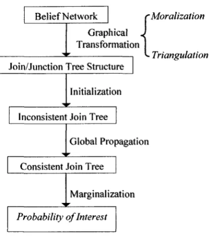
Figure 2-6 Block Diagram of JT Algorithm.

Figure 2.6 shows the block diagram of the JT algorithms. The first step of this

algorithm is to construct the JT from the original Bayesian network. The premises

underlying the construction of JT is that, while the overall problem is too large for

calculating and updating probabilities, the individual clusters are of manageable size. The

general idea behind this is that because of the representation, the propagation of evidence

through the network can be carried out more efficiently. JT based propagation algorithm

is also referred to as the fastest algorithm for most applications in the literature [Chl991].

JT based propagation algorithm consists of four steps: (1) transforming a BN into

a junction tree, (2) initializing the clusters of the JT to from cluster potential, (3)

propagating potentials in the network, and (4) answering a query. These steps are

(33)

2.5.1 Junction tree from Bayesian network

1. Moralization

In the moralization step, a directed acyclic graph (or DAG) is converted into an

undirected graph, so a uniform treatment of directed and undirected graphs is possible. A

moral graph is obtained by linking the parents of each node and dropping the

directionality of the edges in DAG.

2. Triangulation

The triangulation step determines the "elimination" order of the graph.

Triangulation means looking at the undirected graph for cycles from a variable to itself

going through a sequence of other variables. Triangulating a graph means there should be

no cycle in that graph with length greater than three. It is done by adding undirected

edges so that there are no such cycles. Triangulation is essential to producing clusters of

variables that are trees. Finding the "best" triangulation is NP-hard [MR2006].

3. Construct the junction tree

Given a triangulated graph, a junction tree is constructed by forming a maximal

spanning tree (a tree of a connected graph composed of maximal set of edges but contains

no cycle) from the clusters in that triangulated graph. A cluster tree (is a tree where nodes

are cluster and there is a single path between every pair of clusters) is constructed with

separators. A cluster tree is a junction tree if and only if it has the running intersection

property of the junction tree properties.

(34)

fd) Sl2

\ s I \~s T V_^ -j

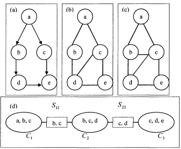
Figure 2-7 (a) A simple BN. (b) The Moral Graph, (c) The Triangulated Graph.

(d) JT is constructed.

Figure 2-7 shows all the steps of construction of the JT from a simple BN i.e.

figure 2-7(a). As of first step, during the moralization shown in figure 2-7(b), the BN is

first converted into an undirected graph (by removing arrow heads) and then the parents

of node e is joined as they are not joined before. The next step is triangulation which is a

representation based on a number of maximally connected subgraphs (figure 2-7(c)),

which formed the basis of the local representation, and are connected such that the global

properties (parent-child relationships and the potential of the BN) are preserved.

After the triangulation is done, clusters are formed as

C, =(a,b,c),

C2=(b,c,d),

C3 = (c,d,e).

The ordering of edges is achieved by considering their position in the original DAG,

(35)

cluster and connects this to the predecessor cluster which shares the largest number of

common nodes and so on. If two clusters share some variables, then the edge connecting

them carries that variable, called separator. Hence the JT is formed as in figure 2-7(d).

After the construction of the DAG, each cluster in this representation is associated

with a cluster potential and this step is known as initialization in the JT algorithm.

2.5.2 Initialization on the Junction tree

After the JT is built, the initialization phase of the HUGIN architecture sets up the initial

potentials for the clusters of the JT. In particular, the CPD of each node from the original

BN is assigned to a cluster that possesses the node itself and its parents. Then, within

each cluster, these CPDs assigned are multiplied together to form one single potential for

the cluster i.e. the set of CPDs p(x | Fx) associated with a cluster C, are in standard JT

architectures combined to form the initial cluster potential <I>, as:

The potentials of separators are initialized to unity.

The initialization step proceeds as follows [HDarl996]:

• For each separator Si, assign potential with values equal to 1: Ons7 <- 1.

• For each random variable x in U, perform the following:

o Assign to a cluster C, that contains x and family of x; call Ft (also call

the parent ofx). The potential of the cluster will be:

OT<-^f''.p(.x\F

x

).

o If x and Fx is a subset of two or more clusters, then arbitrarily assign the

CPD ofx, i.e. p(x | Fx)to one of the clusters.

(36)

EXAMPLE of Initialization in JT:

p(h) p{c I h) p{t | c)

C,

c,h

pic | h).pih)

C-,

t,c

(a) (b)

Figure 2-8 (a) The BN. (b) Corresponding JT with initialized CPDs.

Figure 2-8 (a) shows a simple BN and the corresponding JT for this BN is

presented in figure 2-8 (b). The JPD of the given BN is:

pic,h,t) = pic | h).pih).pit | c). (1)

In the JT, each cluster {C^C2} has two nodes from the original BN i.e.

C, = {c,h} and C2 = {t,c}, and the edge between them contains the common node of the

two clusters i.e. Su = {c}. According to initialization procedure, CPD for node h, i.e.

pih) is assigned to cluster C, where it is itself present and CPD for node c i.e. pic \ h)

is also assigned to cluster C, as the node itself and its parent (i.e. node h from the

original BN in figure 2-8(a)) both are present in cluster C,. Following the same

procedure CPD for node / i.e. pit \ c) is assigned to cluster C2. So the potentials for

cluster C, and C2 are

<J>, <- pic | h).pih) and

<D2 < - / ? ( c / | c ) .

And the potential for the separator Sn is assigned to 1, i.e. 012 <—1 . The joint probability distribution over all the variables is simply the product of cluster potentials,

i.e.

(37)

which is exactly the global property i.e. JPD which is obtained (equation (1)) from the

original Bayesian network given in figure 2-8(a).

After the initialization step, message propagation step transforms the cluster

potentials into cluster marginals. One of the prime applications of the propagation

algorithms in Bayesian networks is to evaluate marginal distributions of variables,

perhaps conditional on values (evidence, findings) of some other variables in the

network.

2.5.3 Message Propagation on the Junction tree

A cluster from which propagation starts is called as root cluster. The JT based algorithm

can be regarded as proceeding by the propagation of messages through the junction tree,

involving only two adjacent edges. The core step is message propagation which consists

of two phases of operation. Computations are done by each cluster and by each separator

in the junction tree [LeShl998] where each cluster and each separator in the junction tree

stores a potential. At all times the joint potential is equal to the product of the potentials

at the clusters divided by the product of the potentials at the separators. The basic

operation for message propagation between clusters in a JT is called absorption.

c,

(

a

V

v y

p(c | h).p(h)

Sn

c

1

c,

- r i o

pit | c)

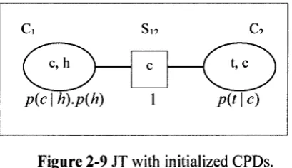
Figure 2-9 JT with initialized CPDs.

For example, in figure 2-9, the cluster C2 absorbs from the cluster C, as follows:

The potential p(c \ h).p(h) at C, is reduced (through the marginal operation) to a

(38)

which updates its own potential to the product/?(/1 c).p{c). Note that, before the

absorption, neither p(c) nor p{t) can be obtained at the cluster C2. However, after the

absorption, both of them can be computed locally atC2.

With the propagation phases the junction becomes consistent with each cluster

containing the joint probability distribution for the variables it contains. In JT based

probabilistic model, we make inferences by computing the marginal of the joint

probability distribution for the variables of interest.

2.6 Message Propagation Schemas

A message propagation scheme is used to compute the marginals. Queries can then be

answered very fast. By using junction trees as the computational structure, in the

uncertain reasoning literature, there are three well known architectures for message

passing on the junction tree. They are:

o The Shenoy-Shafer Architecture [SS1990],

o The Lauritzen-Spiegelhalter Architecture [LSI988],

o The HUG1N Architecture [JOL1990].

Each of these architectures has a junction tree as underlying computational

structure. There is no big difference between the Lauritzen-Spiegelhalter Architecture

and the HUGIN Architecture. On the other hand, Lauritzen-Spiegelhalter showed that

HUGIN is more computationally efficient than Lauritzen-Spiegelhalter's architecture

[LeShl998]. Thus the HUGIN and Shenoy-Shafer architectures are the two variations for

message passing on the junction tree based algorithm, which exhibit different tradeoffs

with respect to efficiency and query answering power. Lauritzen et al. [LSI988] and

Jensen [JLO1990] described HUGIN as one of the efficient inference engine for

computing posterior probability based on observed evidence. Park and Darwiche

[ParDar2003] also claimed that HUGIN architecture is more time-efficient than the

(39)

In order to improve the efficiency of the HUGIN architecture, many modifications

have been done by researchers [Dawl992], [SchS1998], [ParDar2003], [BZKPC2006].

Recently, by utilizing the semantic meaning of message passing, with allocate separator

marginal (ASM) procedure; Wu and Jin [WuJ2006] were able to pass much lesser

number of messages than that of by HUGIN. They investigated the message passed

algebraically, and by using the semantics of the messages they revealed that the messages

passed are not mere potentials, but in fact separator marginals or factors in their

factorizations.

For this thesis, we have taken HUGIN architecture as our basis to improve the

performance of the junction tree based propagation algorithms, as this architecture is

considered as the efficient architecture for computing belief in JT. As ASM procedure

improves the performance of HUGIN architecture by lowering the number of message

passing required by HUGIN, HUGIN architecture and ASM procedure are the grounds

on which this thesis is focused. These two approaches are explained in the following

subsections.

2.6.1 HUGIN Architecture

After the construction of the JT and initialization phase, in the HUGIN architecture each

separator holds a single potential over the separator variables which initially is a unity

potential. During propagation phase the separator and cluster potentials are updated.

The HUGIN architecture performs probabilistic inference by passing messages

around JT and propagating the global effects of local information. Because the clusters

share nodes with its neighbors, consistent probability measures must be obtained. Thus

global properties (for example, JPD of the original BN) are preserved while computation

can proceed on local subgraphs (i.e. clusters of JT). Thus the propagation method for

(40)

(GP) method [SAS1994], [HDarl996]. The GP method used in the HUGIN architecture

is arguably one of the best methods for probabilistic inference in Bayesian networks

[HDarl996].

Then the GP method begins by choosing an arbitrary cluster as root. A root

cluster is the one with which propagation starts. A JT with n clusters performs 2 x (n -1)

message passes starting from the leaves, divided into two phases. When a cluster receives

messages from all its neighbors except that one towards the root, it is allowed to send a

message upwards, and so on until the root cluster has received messages from all its

neighbors. This is called the COLLECT-EVIDENCE. Now the root cluster sends a

message to all its neighbors, and every cluster receiving a message itself, sends another

one to all its neighbors except the one from which received the message, and so on until

the leaves are reached. This last phase is called DISTRIBUTE-EVIDENCE. When a

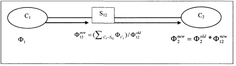
cluster C, passes a message to cluster C2 (or C2 absorbs the message from C,) it means a two-step computation:

(1) Updating the separator cluster On by setting 0>"2CT' = ( £ Q_Su 0C | )/q>£ ; (2) Updating the cluster potential Q™ = <Df * O™".

The potential <DI2 is the so-called "message" passed from cluster C, to cluster C2

in the JT. Obviously, <bn in general is just a non-negative function. The sequence of the

single message pass is shown in figure 2-10.

r^^

\ l )

S12

°i,2'"=(Zc1-.s-,2<l>r,)/<

(

A

^new

v2 ^ 1 2

(41)

The result of global propagation is that each cluster passes its information to all

other clusters in the cluster tree. A cluster can only pass a message to a neighbor after the

cluster has received messages from all of its other neighbors [Dawl992]. This ensures

consistency of the cluster tree when global propagation is completed. Marginal

probabilities for individual variables can then be obtained from the clusters.

HUGIN architecture needs to send 2 x (n -1) (where n is the number of clusters

in the JT) number of messages to achieve the consistency of the JT. But by utilizing the

semantics of the messages with allocate separator marginals (ASM) procedure Wu and

Jin [WuJ2006] successfully avoided passing up to half of the messages that could have

had to be passed by the GP method. This procedure is explained in the next section.

2.6.2 Allocate Separator Marginal (ASM) Procedure

By studying the factorizations of a JPD defined by a BN before and after the GP method

is performed, Dan Wu and Karen Jin [WuJ2006] investigated the messages passed

algebraically, and revealed that the messages passed are separator marginals or factors in

their factorizations. By utilizing the revealed semantics of the messages they successfully

avoided passing up to half of the messages that could have had to be passed by the GP

method. They named the procedure as 'Allocate Separator Marginals' (ASM)

[WuJ2006].

For any random variable x, in U = {x,,..., xn} in a BN,

Step 1. Suppose the CPD of x, i.e. /?(x, \ Fx) is assigned to a cluster Ck to form <Dt. If the variable x, appears in a separator Skj between Ck and Cy, then draw a small arrow originating from xt in the separator Skj pointing to the cluster C.. If variable x, also

(42)

separators and point to the neighboring cluster away from cluster Ck 's direction. Repeat

this for each CPD p{x, \ Fx) where /' = {l,...,n} of the given BN.

Step 2. Examine each separator Stl in the junction tree, if the variables in Stj all pointing

to one neighboring cluster, then the separator marginal piS^) will be allocated to that

neighboring cluster otherwise, p(St/) has to be factorized so that the factors in the

factorization can be assigned to appropriate cluster indicated by the arrows in the

separator.

The Result of applying the ASM procedure to the junction tree will be:

> If all variables in the same separator are pointing to the same neighboring cluster,

that means the separator marginal as a whole (without being factorized) will be

allocated to the neighboring cluster. And during the propagation phase if p{Stj)

as a whole is allocated to C., then message mi_yj = p(Sy) and m(<_y = 1.

> If the variables in the separator are pointing to different neighboring clusters, that

means the separator marginal has to be factorized before the factors in the

factorization can be allocated according to the arrow, i.e. if p(Sy) has to be

factorized (following a topological ordering of variables in Stj), then ml^j = the

product of factors allocated to Cj and /w, . = the product of factors allocated

toC,.

Thus one cluster only needs to multiply the originally assigned CPDs of a cluster

with the allocated separator marginal(s) or the factors in its (their) factorization(s)

suggested by the procedure ASM, in order to obtain the cluster marginal. The other

messages passed by the GP method are identity as function 1, which has no effect on the

receiving clusters. This approach of ASM helps to save at most half number of messages

(43)

EXAMPLE ASM Procedure:

p(ajQ { b )

p

(b)

p{e\b)

P(h\f) P(f\c,d) Pfert'f)

p(a), p(c | a) p{d), p(d \ b), p(e \ b)

Mr.

P(c\

P(f\cdji

crlf

P(f}

df

P(f\d)

J I

de \p(de)

d e f

P(h\£L

fh

e f > ( e / )

1 efp j p ( g | e / )

fa) fb) Figure 2-11 (a) A BN. (b) JT with initialized CPDs.

Figure 11(a) shows a simple BN and the corresponding JT is given in figure

2-11(b). The procedure ASM is illustrated using Figure 2-2-11(b).

During the initialization phase, the CPD of c i.e. p(c \ a) is assigned to a cluster

Cac to form <I>C (ac). The variable c appears in a separator between Cac and Ccdf, so by

following the ASM procedure, a small arrow is drawn originating from Cac in the

separator Sc pointing to the cluster Ccdf. Following the same rule, CPD for variable /

will be assigned to Cfh. As variable / appears in more than one separators in the

junction tree, so a small arrow will be drawn from those separators and point to the

neighboring cluster away from cluster CJh 's direction.

Now if all variables in the same separator are pointing to the same neighboring

cluster, that means the separator marginal as a whole (without being factorized) will be

(44)

p(ef) (figure 2-11(b)) will be allocated to cluster C{cdf),C{def) and C(efg) respectively.

But if the variables in the separator are pointing to different neighboring clusters, that

means the separator marginal has to be factorized before the factors in the factorization

can be allocated according to the arrow. For example, the separator marginal p(df) has

to be factorized so that the factor p(d) is allocated to cluster C(cdf) and p(f \ d) will be

allocated to cluster C(def).

The separator marginal p(df) is decomposed as p(df) = p(d).p(f \d). It is

important to note that the factorization p(df) = p(d).p(f \ d) does not follow the

topological ordering of the variables d and f (d should precede / in the ordering)

with respect to the original DAG, in which / is a descendant of d.

Now from the figure 2-11(b) (arrows indicates the direction of the messages) we

can see that after only 8 message passes the cluster potential will become cluster

marginal, on the other hand with the GP method of HUGIN, 2 x (6-1) = 10 message

passes were needed to achieve the marginality of cluster. Thus ASM procedure saves 4

message passes that needed to be passed by the HUGIN architecture.

2.7 Marginality of Clusters

A typical application of probabilistic inference involves constructing a probabilistic

model, such as a Bayesian network, and then applying algorithms to the model to

compute answers to probabilistic queries. Probabilistic inference consists of computing

probabilities that are not explicitly stored by the reasoning system, such as computing

marginal and conditional probabilities from the joint probability distribution.

The main goal of message passing is to transform the cluster potentials into

cluster marginals after assigning all the CPDs from the original BN to an appropriate

(45)

Bayesian factorization into a marginal factorization [WWu2004]. Also in probability

theory and statistics, the marginal distribution of a subset of a collection of random

variables is the probability distribution of the variables contained in that subset. .

According to the Global Propagation (GP) method in the traditional HUGIN

architecture, during the time of initialization, with the assignment of CPDs, every cluster

in the junction tree is associated with a cluster potential. During the course of

propagation, after receiving all messages from its neighbors, these cluster potentials

transform into cluster marginals. Thus HUGIN architecture needs 2 x (n -1) messages to

obtain the marginality of a cluster. . But with the ASM procedure, Wu and Jin revealed

that, the product of the messages received by every cluster in the GP method equals to the

product of all separator marginals. Thus one cluster only needs to multiply the originally

assigned CPDs of a cluster with the allocated separator marginal(s) or the factors in its

(their) factorization(s) suggested by the procedure ASM in order to obtain the cluster

marginal. This approach of ASM helps to save at most half number of messages that

Heuristic assignment of CPDs for probabilistic inference in junction trees

Scholarship at UWindsor

Scholarship at UWindsor

Heuristic assignment of CPDs for probabilistic inference in

Heuristic assignment of CPDs for probabilistic inference in

junction trees

junction trees

Heuristic Assignment of CPDs for Probabilistic Inference in

Junction Trees

1*1

AUTHOR'S DECLARATION OF ORIGINALITY

ABSTRACT

TABLE OF CONTENTS

LIST OF TABLES

1. INTRODUCTION

2. BACKGROUND

©

of

x

©

GMD

c.d~h

OT<-^f''.p(.x\F

).

c,

(

a

V

v y

c,

- r i o

r^^

A

p(ajQ { b )

(b)

P(h\f) P(f\c,d) Pfert'f)

P(f\cdji

P(f}

P(f\d)

J I

**1*1**