INVESTIGATION
Peak and Persistent Excess of Genetic Diversity
Following an Abrupt Migration Increase
Nicolas Alcala, Daniela Streit, Jérôme Goudet, and Séverine Vuilleumier1
Department of Ecology and Evolution, Biophore, University of Lausanne, CH-1015 Lausanne, Switzerland
ABSTRACTGenetic diversity is essential for population survival and adaptation to changing environments. Demographic processes (e.g., bottleneck and expansion) and spatial structure (e.g., migration, number, and size of populations) are known to shape the patterns of the genetic diversity of populations. However, the impact of temporal changes in migration on genetic diversity has seldom been considered, although such events might be the norm. Indeed, during the millions of years of a species’lifetime, repeated isolation and reconnection of populations occur. Geological and climatic events alternately isolate and reconnect habitats. We analytically document the dynamics of genetic diversity after an abrupt change in migration given the mutation rate and the number and sizes of the populations. We demonstrate that during transient dynamics, genetic diversity can reach unexpectedly high values that can be maintained over thousands of generations. We discuss the consequences of such processes for the evolution of species based on standing genetic variation and how they can affect the reconstruction of a population’s demographic and evolutionary history from genetic data. Our results also provide guidelines for the use of genetic data for the conservation of natural populations.
G
ENETIC diversity in a population of constant size results from the balance between the occurrence of new muta-tions and the loss of alleles by genetic drift (Fisher 1922; Wright 1931; Kimura and Crow 1964). The expected pop-ulation genetic diversity can thus be estimated from the effective population size and the mutation rate in the pop-ulation. In subdivided populations this estimate should fur-ther account for the strength of migration (Maruyama 1970; Smith 1970; Nei 1973): limited migration allows for strong differentiation between populations, while strong migration tends to homogenize genetic diversity between populations. Genetic diversity is also known to be affected by population demographic changes; following bottlenecks and founder events, a loss of genetic diversity is expected to occur (Neiet al. 1975). Recently, spatial population expansions were shown to lead to increased differentiation between popula-tions and to generate a low level of genetic diversity at the front of the expansion (Excoffieret al.2009).
Although theoretical studies on the dynamics of genetic diversity in subdivided populations started appearing in the
1970s (Nei and Feldman 1972; Latter 1973; Nei 1973; Nagylaki 1974, 1977), the transient dynamics and nonequi-librium states of genetic diversity still do not have a good theoretical basis. Early authors characterized the ultimate rate of change of genetic diversity after a perturbation (ei-ther a change in population size or geneflow; Nei and Feld-man 1972; Latter 1973; Nei 1973; Nagylaki 1974, 1977). They found that changes in genetic diversity are related to the total effective population size, which results in a slow dynamics of genetic diversity change. They thusfirst high-lighted that nonequilibrium states and transient dynamics are expected to act on very large temporal scales. In partic-ular, they showed that decreases in migration rates (popu-lation fragmentation or iso(popu-lation) have long-term effects on genetic diversity: they reduce the amount of genetic diver-sity within populations and allow for population differenti-ation (Latter 1973; Takahata and Nei 1985). Additionally, it has been shown that short timescale randomfluctuations in migration increase population differentiation (Nagylaki 1979; Whitlock 1992; Rice and Papadopoulos 2009) while cyclic fluctuations of gene flow (such as seasonal fl uctua-tions) mainly affect genetic diversity within populations (Karlin 1982; Shpaket al.2010). Although the genetic con-sequences of migration events (admixture) have recently received much attention (e.g., Pritchardet al.2000; Falush
et al.2003; Priceet al.2009; Gravel 2012), their impact on
Copyright © 2013 by the Genetics Society of America doi: 10.1534/genetics.112.147785
Manuscript received August 27, 2012; accepted for publication December 26, 2012 Supporting information is available online athttp://www.genetics.org/lookup/suppl/ doi:10.1534/genetics.112.147785/-/DC1.
genetic diversity and more particularly the expected induced transient dynamics have not received much attention.
Genetic diversity has a crucial importance in estimating populations at risk of extinction and species’adaptive poten-tial. Current genetic diversity characterizes species at risk of extinction through inbreeding depression, loss of genetic di-versity, and accumulation of deleterious mutations (Gilpin and Soule 1986; Jimenez et al. 1994; Frankham 1995; Hedrick and Kalinowski 2000). The current level of genetic diversity (or standing genetic variation) is now widely rec-ognized as a determinant for the adaptation of a population to a novel environment (Turner et al. 1993; Feder et al.
2003; Pelz et al. 2005; Colosimo et al. 2005; Hermisson and Pennings 2005; Myles et al. 2005; Hernandez et al.
2011; Jones et al. 2012). First, under new selective pres-sures, the adaptive value of a preexisting allele can switch from neutral or deleterious to beneficial (Gibson and Dworkin 2004; Hermisson and Pennings 2005). Second, alleles from the standing genetic variation are present at higher frequen-cies in the population than any newly arisen (de novo) muta-tion are; thus, they have higher fixation probabilities and lower times tofixation (Barrett and Schluter 2008). Finally, these alleles have already passed successive selective filters and are consequently more likely to be compatible with the background genome (Orr and Betancourt 2001; Schluter
et al.2004; Barrett and Schluter 2008).
Measures of genetic diversity are widely used to un-derstand and infer the demographic and evolutionary history of populations. Indeed, statistical tests using poly-morphism data can detect departure from neutrality and infer demographic or selective processes (e.g., Ewens 1972; Watterson 1978; Tajima 1983; Fu and Li 1993; Fay and Wu 2000; see review in Kreitman 2000). Furthermore, due to recent modeling advances in coalescent theory and in-creased genomic data and computational power, it is now possible to distinguish different demographic scenarios (e.g., population bottleneck and subdivision; Peter et al. 2010) and estimate demographic and selective parameters (e.g., populations size and growth rate, proportion of admixture, selection coefficient) using polymorphism data (Beaumont
et al.2002; Kim and Stephan 2002; Kim and Nielsen 2004; Nielsen et al. 2005; Price et al. 2009). Nevertheless, it is often difficult to distinguish between the transient effects of demographic changes and the effects of selection on poly-morphism data (Jensen et al. 2005; Nielsen 2005; Li and Stephan 2006; Kim and Gulisija 2010; Pavlidiset al.2010). It is also difficult to distinguish between the signatures of different demographic changes such as changes in popula-tion size, number, or migrapopula-tion rate (Wakeley 1999). A bet-ter understanding of the impact on genetic data of transient dynamics during demographic changes is necessary to dis-entangle these processes.
Interestingly, although the impact of population subdi-vision and short timescale population demographic changes on genetic diversity have received a lot of attention, other processes, such as long-term isolation and subsequent
population reconnection, have received little attention. Such events have, without a doubt, occurred several times in the past, at long and short timescales. Repeated environmental changes have modified habitats and species distribution and created isolation and reconnection of populations. For example, during the climatic oscillations of the Quaternary period, temperate and tropical species were successively isolated into refugia and experienced habitat and population expansion, allowing for population reconnection (Hewitt 2000, 2004; Zhang et al.2008; Younget al.2009). At the same time, the reduction of sea levels (120 m lower than present; Lambecket al.2004) allowed the formation of land bridges that connected isolated lands in several parts of the world (Hewitt 2000). Repeated changes in water level resulted in fragmentation and fusion of basins within con-tinents (as in the Great African Lakes; Galis and Metz 1998; Sturmbaueret al.2001). Similarly, geological events such as volcanic eruptions induced periodic isolation and reconnec-tion of islands (Cook 2008), while tectonic processes such as the formation of mountains isolated populations and recon-nected others (Hughes and Eastwood 2006; Antonelliet al.
2009; Antonelli and Sanmartín 2011). More recently, cli-matic, environmental, and anthropogenic changes (e.g., global warming, urbanization, and agriculture) have also played important roles in modifying the connectivity pattern between populations (Miller and Hobbs 2002; Delaneyet al.
2010). Consequently, some species are currently subdivided into poorly connected or completely isolated populations; for examples, ground beetles (Kelleret al.2004), salamanders (Noel et al. 2007), and crickets (Vandergastet al. 2009). In the meantime, other species experience habitat and population expansion (e.g., sparrows, white-tailed deer, zebra mussels; Waples 2010). Isolation and reconnection of populations not only reflect abiotic processes, but they can also represent spatial and temporal interactions of popula-tions (e.g., secondary contacts; Greenet al.2010; Domingues
et al.2012). Consequently, transient states of genetic diver-sity are expected to be the norm and deserve much more attention.
species diversity and how they can affect the reconstruction of populations’demographic and evolutionary history from genetic data.
Genetic Diversity of Populations
To study the dynamics of genetic diversity after connectivity changes, we consider diploid individuals in a finite island model composed ofnrandom mating populations of sizeN, so that the total population size is nN. The populations ex-change migrants at a ratem. The mutations follow the infi n-ite allele model (each mutation produces a new allele; Kimura and Crow 1964) and occur at a ratem. The gener-ations are nonoverlapping (Wright–Fisher model; Fisher 1930; Wright 1931).
Genetic diversity, H, is estimated using the identity-by-descentFbetween pairs of alleles, through the relationship provided by Nei and Feldman (1972):
H¼12F: (1)
Further, we characterize within-population genetic diversity
Hs and between-population genetic diversity Hb, using
within- and between-population genetic identities, respec-tively. Within-population genetic identity, Fs, corresponds
to the probability that two genes randomly chosen from the same population are identical by descent. Between-population genetic identity,Fb, corresponds to the probability that two
genes randomly chosen from different populations are identical by descent. Considering that within- and between-population genetic identitiesFsandFbat a given timetare, respectively, Fs,tandFb,t, their values at the next generation (forward in time), respectively, Fs,t+1 and Fb,t+1, will follow (Smith
1970; Maruyama 1970; Latter 1973)
Fs;tþ1¼
acþ ð12cÞFs;t
þ ð12aÞFb;t
ð12mÞ2
Fb;tþ1¼
bcþ ð12cÞFs;t
þ ð12bÞFb;t
ð12mÞ2; (2a)
where the parameters are
a¼ ð12mÞ2þ m
2
n21 (2b)
b¼ 12a
ðn21Þ (2c)
c¼ 1
2N: (2d)
System of Equations 2 can be expressed under matrix notation as
Ftþ1¼AFtþB; (3a)
where
A¼ ð12mÞ2
að12cÞ 12a bð12cÞ 12b
(3b)
B¼ ð12mÞ2
ac bc
(3c)
Ft¼
Fs;t
Fb;t
: (3d)
Parameters have the following interpretation:ais the prob-ability that two genes at the same location before migration are still at the same location after migration (either both migrate to the same location or both do not migrate);b is the probability that two genes that were at the same location before migration migrated to different locations; c is the probability that two genes within a population are copies of the same gene; and (12m)2is the probability that
nei-ther of the two randomly chosen genes mutated.
Predicting the Dynamics of Genetic Diversity
To characterize the impact of connectivity changes on genetic diversity, we analyzed the trajectories of within- and between-population genetic identities from any initial genetic identity state. Using Equation 2, Smith (1970) and Maruyama (1970) showed that genetic identities converge toward an equilibrium value Feq (value given in Supporting Information, File S1).
Extending the results obtained by Nei and Feldman (1972) forn = 2 populations, we show that the temporal dynamics of genetic identities follow (see Appendix A for more details)
Ft¼C1lt1þC2lt2þFeq; (4a)
where
Feq¼
Feqs
Feqb
: (4b)
l1andl2are respectively the largest and smallest eigenval-ues of matrixA, and they follow
l1¼ð
12mÞ2 2
að12cÞ þ12bþ
ffiffiffiffiffiffiffiffiffiffiffiffiffiffiffiffiffiffiffiffiffiffiffiffiffiffiffiffiffiffiffiffiffiffiffiffiffiffiffiffiffiffiffiffiffiffiffiffiffi
ð12að12cÞ þbÞ224bc
q
l2¼ð
12mÞ2 2
að12cÞ þ12b2
ffiffiffiffiffiffiffiffiffiffiffiffiffiffiffiffiffiffiffiffiffiffiffiffiffiffiffiffiffiffiffiffiffiffiffiffiffiffiffiffiffiffiffiffiffiffiffiffiffi
ð12að12cÞ þbÞ224bc
q
:
(5)
C1andC2are column vectors of dimension 2 composed of
constant values, which depend on the parameters of the model (m,m, n, and N) and on the initial genetic identity
F0(Appendix A).
In the next section, we provide from Equations 4a and 5 the temporal change of genetic diversity and derive the corresponding time to reach genetic diversity equilibrium after a connectivity change.
Time to Reach Genetic Diversity Equilibrium
dynamics. Indeed, the temporal change of genetic diversity depends on two components: jC1lt1j and jC2lt2j(Equation
4a). They both follow an exponential decay and their rate of change depends onr1= ln(l1) andr2= ln(l2), respectively
(Appendix A). As 1 . l1 . l2 . 0, jC2lt2j decays more
rapidly than jC1lt1j (see Appendix A). Thus r1 determines
the ultimate (or long-term) change of genetic diversity and
r2 determines the transient (or short-term) change of
ge-netic diversity.
When migration and mutation rates are small (i.e.,m1 andm 1) and local population sizes are large (i.e.,N
1), the decay constantsr1andr2follow
r1¼ 22m2 1 2Ne
r2¼ 22m22m n n212
1 2Nþ
1 2Ne
(6a)
with
Ne¼nN
1þðn21Þ
nM
; (6b)
where M= 4Nmis the scaled migration rate andNeis the
effective population size of the total population (inbreeding, eigenvalue, variance, and mutation effective size are equiv-alent in thefinite island model; Whitlock and Barton 1997). As expected from theory (Whitlock and Barton 1997; Wake-ley 1999), in the strong migration limit (M1), the effec-tive size is equal to the total population sizenN, while in the weak migration limit (M 1), the effective size is higher than the total population size.
We can estimate the durations of the ultimate and transient changes of genetic diversity, denotedt1andt2,
re-spectively. Formally, we define t1 and t2 as the times (in
number of generations) needed forlt1andl t
2 to be reduced
to a numbera, wherea2]0; 1]:
lt1
1 ¼a
lt2
2 ¼a:
(7)
Assuming that migration and mutation rates are small and population sizes are large, t1and t2simplify to (Appendix
A):
t1¼ 2
lnðaÞ 2mþ1=2Ne
t2¼ 2
lnðaÞ
2mþ2mðn=ðn21ÞÞ þ1=2N21=2Ne
(8)
The genetic diversity changes as follows (Figure 1): (i) a convergence of duration t2from the initial genetic
diver-sity value to a transient genetic diverdiver-sity value and then (ii) a convergence of durationt1to the genetic diversity
equilib-riumHeq. The time to reach genetic diversity equilibrium,t 1,
depends only on two terms: the mutation rate (term 2m)
and the genetic drift at the total population level (term 1=2Ne). The duration of the transient dynamics,t2, depends
on four terms: the mutation rate (term 2m), the migration rate (term 2m), the genetic drift in each population (term 1=2N), and the genetic drift at the total population level (term 1=2Ne). The convergence to the transient and
equilib-rium values of genetic diversity can occur on separated time-scales (i.e.,t1t2) depending on the parameter values. The
timescalest1andt2can differ from several orders of
magni-tude. Whenn.14, differences are the highest (t1t2), in
the domain wherem1=2Nand also whenm1=2Nand
m.m. Whenn#14, the same conditions apply fort1t2
except in a restricted domain wherem’1=2N(see Appen-dix A). For example, the duration of the transient dynamics is t2’134 and the time to reach equilibrium ist1’1.5·
105generations (witha= 5%), when 10 populations of size
2500 with a mutation rate of 1026are connected with a
mi-gration rate of 0.01.
Dynamics of Genetic Diversity After an Isolation Event
We analyzed the dynamics of genetic diversity after an isolation event, starting with a situation in which popula-tions are connected and at their equilibrium value; i.e., within- and between-population genetic diversity Hs and Hbare at the expected connection equilibrium valuesHseq;con
andHbeq;con (see Maruyama 1970; Smith 1970; andFile S1).
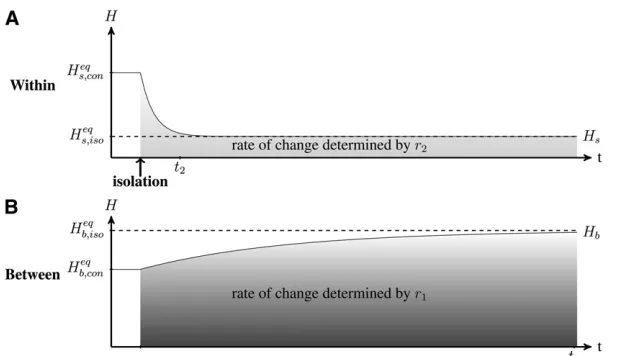
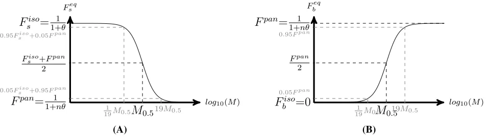
We observe (Figure 2) that immediately after an isolation event, within-population genetic diversity decreases due to genetic drift to the point where it reaches the mutation-drift equilibrium of an isolated populationHseq;iso(seeFile S1and Kimura and Crow 1964), at a rate determined byr2(from
Figure 1 The time (in number of generations)t1to reach genetic diversity
equilibrium and the length of the transient dynamics periodt2as a
func-tion of the migrafunc-tion ratem. The solid line corresponds ton= 2 popu-lations, the dashed line ton= 10, and the dotted line ton= 100.t1is
always at least one order of magnitude higher thant2. This separation of
the two periods becomes even greater whenm>1=4N¼1024.
Equation 6). Meanwhile, between-population genetic diver-sity slowly increases due to the differentiation of popula-tions induced by mutapopula-tions (at a rate determined by r1
from Equation 6). Populations ultimately reach complete differentiation (equilibrium value of Heqb;iso¼1). We can show from Equation 2 that following an isolation event, within- and between-population diversities change indepen-dently and reach their equilibrium value int2andt1
gener-ations, respectively (File S2).
The decrease of population genetic diversity (within) can occur quickly relative to population differentiation (between-population genetic diversity; see Figure 1). After an isolation event, within-population genetic diversity (Hs)
remains above its expected equilibrium Heqs;iso, while
be-tween-population genetic diversity (Hb) remains below its expected equilibriumHbeq;iso. However, the timescales of these
nonequilibrium periods differ. When populations are iso-lated (m= 0), Hs reaches a value close to its equilibrium
value int21=ð2mþ ½1=2NÞgenerations, whileHbreaches
a value close to its equilibrium value in t1 1=2m
genera-tions (Equation 8). Therefore, when 2m1=2N, Hs
con-verges much more quickly thanHb, and when 2m1=2N,
both converge in approximately the same amount of time. For example, assuming m = 1025 and N = 1,000, H
b is
significantly lower than the equilibrium value for approxi-mately t1 ’ 150,000 generations while Hs is significantly
higher than the equilibrium value for approximately t2 ’
6000 generations (givena= 5%).
Dynamics of Genetic Diversity After a Connection Event
We analyzed the dynamics of genetic diversity after a con-nection event, starting with a situation in which populations are isolated and at their equilibrium value Heqs;iso andHbeq;iso
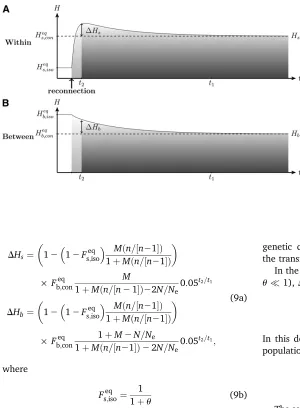
(see Smith 1970; Maruyama 1970 andFile S1). After a con-nection event (Figure 3), the genetic diversity accumulated in each population during the isolation period is quickly
spread to all populations (Figure 3, fast dynamics in light shading, at a rate determined by r2 from Equation 6).
Consequently, within-population genetic diversity quickly increases and reaches a high value that is above its ex-pected connected equilibrium value (Heqs;con, Figure 3; see File S1). This process creates a peak of within-population genetic diversity DHs and a transient excess of genetic diversity between populationsDHb(see Figure 3). Then,
due to genetic drift, both the within- and the between-population diversities decrease (slow dynamics in dark shading in Figure 3, at a rate determined by r1 from
Equation 6), to the point where the diversities reach the expected value of mutation–migration–drift equili-brium (Heqs;con and Heqb;con from Equation 4b; Kimura and
Crow 1964).
Within- and between-population diversities change suc-cessively according to two timescales: first, a fast transient dynamics, followed by a slow asymptotic dynamics (sepa-ration of timescales is derived in Appendix A and illus-trated in Figure 3). Because the transient dynamics can be shorter than the asymptotic dynamics, the excess of ge-netic diversity (DHsandDHb) can be maintained for a very
long period (from Figure 1, t1 is longer than 10,000
generations).
Peak of Genetic Diversity Generated by a Connection Event
In this section, we characterize the peak of within-population genetic diversity, DHs, and the excess of
be-tween-population genetic diversity, DHb, observed after
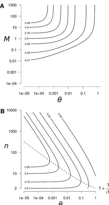
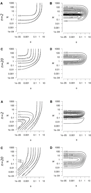
a connection event as a function of the mutation rate, the genetic drift, the number of populations, and the mi-gration rate after connection. The exact value of the within-population genetic diversity peak is represented in Figure 4. Assuming that migration and mutation rates are small, we can show that good approximations of the values ofDHsandDHbare (see derivations in Appendix B)
Figure 2 Dynamics of (A) within-populationHs and (B)
between-populationHbgenetic diversity after an isolation
event. Within- and between-population diversity (solid lines) were previously at their respective connection equi-libriumHeq
s;conandHeqb;con. After the isolation event,
within-and between-population diversities reach their isolation equilibriumHeqs;iso andH
eq
b;iso (dashed lines) at rates
deter-mined byr2andr1(Equation 6).t2andt1estimate the time
to reach the within- and between-population genetic di-versity equilibrium, respectively (Equation 8). Under the effect of genetic drift, within-population diversity reaches its equilibrium value faster than between-population ge-netic diversity. Parameters aren= 10,N= 2500,m= 1024
before isolation andm= 0 afterward, andm= 1025.t 1’
149,000 generations andt2’13,600 generations (fora=
DHs¼
12
12Fseq;iso
Mðn=½n21Þ 1þMðn=½n21Þ
· Fbeq;con M
1þMðn=½n21Þ22N=Ne0:05
t2=t1
DHb¼
12
12Fseq;iso
Mðn=½n21Þ 1þMðn=½n21Þ
· Fbeq;con 1þM2N=Ne
1þMðn=½n21Þ22N=Ne0:05
t2=t1; (9a)
where
Fseq;iso¼ 1
1þu (9b)
is the expected equilibrium identity within an isolated population (Kimura and Crow 1964), and
Fbeq;con¼ M
Mþ ðn21Þuð1þuþ ðn=½n21ÞMÞ (9c)
is the expected equilibrium identity between connected populations with the scaled migration rate M, the number of populations n, and the scaled mutation rate u = 4Nm
(Maruyama 1970; Smith 1970). These approximations lead to the largest absolute error when a small number of pop-ulations (n= 2) is combined with weak mutation (u,1) and intermediate migration (M’5). Nevertheless, this er-ror is small (erer-ror,0.025 forDHsand,0.08 forDHb), so
Equation 9 provides a good approximation ofDHsandDHb
for alln,M, anduvalues (see Appendix B for more details about the validity of approximation 9).
The peak of genetic diversity increases with the differ-ence between the two timescales (DHs and DHb increase
witht2=t1) as genetic diversity increases during the transient
phase and decreases during the asymptotic phase. Indeed, when those two phases are separated there is no loss of
genetic diversity caused by the asymptotic decay during the transient phase (terms 0:05t2=t1’1 in Equation 9).
In the domain where the peak is the largest (M1 and
u1),DHsandDHbreach the same value:
DHmax¼n21
n
1
1þnu: (10)
In this domain, DHmaxis maximized when the number of
populations is (dashed line in Figure 4B):
n*¼1þ1=pffiffiffiu (11)
The corresponding peak of genetic diversity, reached atn*, is
DHmaxj
n*¼ 1 1þ2pffiffiffiu:
Interestingly, the number of populations and the peak of diversity have a nonmonotonous relationship. The peak of genetic diversity decreases when the number of populations approaches 2 and when it tends to infinity, while an in-termediate number of populationsn* maximizes the peak of genetic diversity. This can be easily explained by the follow-ing processes. Durfollow-ing isolation, a small number of popula-tions accumulates less between-population genetic diversity; thus, once reconnected, they share a smaller amount of di-versity. In contrast, a large number of populations accumu-lates a higher level of genetic diversity but also has a higher connection equilibrium value; thus, once reconnected, versity reaches its expected equilibrium and no peak of di-versity is observed.
In summary, high peaks of genetic diversity (DHs.0.25
in Figure 4) can occur for a large range of the parameter space: when mutation is weak (u , 0.05) and migration is moderate to strong (M. 0.5). Under these conditions,
Figure 3Dynamics of (A) within-population genetic diversityHs
and (B) between-population genetic diversityHbafter a
reconnec-tion event. Within- and between-populareconnec-tion diversities were pre-viously at their respective isolation equilibriumsHeq
s;iso andH eq b;iso
(Equation 4b). After the reconnection event, within- and be-tween-population diversities reach their respective connection equilibriumsHeq
s;conandHeqb;con(dashed lines). As shown in
Equa-tion 8, the time to reach genetic diversity equilibriumt1and the
length of the transient periodt2are well separated. The two
periods are: (1) fast convergence at a rate determined byr2
(Equation 6) that is driven by the spread of diversity that had accumulated within populations during isolation, which creates the peak of within-population diversity (DHs) and the excess of
between-population diversity (DHb) and (2) slow dynamics at
a rate determined byr1(Equation 6) that is caused by the gradual
loss of genetic diversity. A large number of generations is needed to reach equilibrium. Whenn= 10,N= 2500,m= 1024after
reconnection, andm = 1025,t
1’97,000 generations,t2’
drastic genetic diversity changes can be observed (DHs
values .0.95; Figure 4B forM$50 andu,5·1024).
The number of populations that maximize the peak of diversity, n*, ranges from a few populations when u ’ 1, up to a few hundred populations whenu= 1026
(val-ues of u ,1026 are expected to be very rare, and they
would require a mutation rate lower than 2.5·10212/bp
for a 1-kb gene and a population size of 100). Interestingly, a significant peak of genetic diversity is also observed when only two populations reconnect (DHmax|
n=2 = 0.5; Figure
4B).
Peak of Genetic Diversity Resulting from a Migration Rate Increase
Complete isolation of populations is not required to generate peaks of genetic diversity. Indeed, an abrupt increase of
migration can generate the peak of genetic diversity charac-terized in the previous sections. In File S3, we determined that if migration crosses a threshold valueMT, peaks of
ge-netic diversity can occur. The value of the threshold MT,
as-suming thatm1 andm1, is
MT¼ ðn21Þu 1þu
1þnu: (12)
Consequently, an increase of migration fromM0toM
cross-ing the threshold valueMT(i.e.,M0MT) generates a peak
of genetic diversity that can be approximated by Equation 9 (see File S3). For example, in a subdivided population of
n = 10 andu = 0.1, an increase in migration fromM0=
0.01 toM= 10 (which crosses the migration thresholdMT=
0.495; Equation 12), generates a peak of within-population diversity of 0.350, while a reconnection event in a similar situation would generate a peak of similar intensity (0.358).
Implications for the Inference of Demography and Selection
To describe the impact of migration changes on the in-ference of demography and selection from genetic data, we described the dynamics of two broadly used summary statistics: the Ewens–Watterson statistics (Watterson 1978) and Tajima’sD (Tajima 1989). Both the Ewens–Watterson statistics and Tajima’sDare known to detect an excess (resp. deficit) of rare alleles, which induces negative (resp. posi-tive) values of the statistics, compared with the expected neutral equilibrium (constant size population without selec-tion). Usually, an excess of rare alleles is interpreted either as the signature of balancing selection or population expan-sion, and a deficit of rare alleles is interpreted as the signa-ture of directional selection or as a population bottleneck. We used the Ewens–Watterson statistics, which we denote
HEWand follows (Watterson 1978)
HEW¼Hs2HA; (13)
where Hs is the genetic diversity, and HA is the expected
genetic diversity given the observed number of alleles K. We also used Tajima’sD, which we denoteDT and follows
(Tajima 1989)
DT¼ ffiffiffiffiffiffiffiffiffiffiffiffiffiffiffiffiffiffiffiffiffiffiffiffiffiffiffiffiffiffiffip2S=a1
Varðp2S=a1Þ
p ; (14)
where a1¼
Pm
i¼11=i,lis the sample size, p is the average
number of pairwise nucleotide differences, andSis the num-ber of segregating sites.
We simulated samples of 50 sequences of 1 kb, with a per-nucleotide mutation rate of 2·1028, in four
popula-tions of size 2500, and ran 5000 replicate simulapopula-tions. We simulated an isolation event, where the migration rate changed from 0.002 to 0 and a reconnection event in which the migration rate changed from 0 to 0.002. The simulations
Figure 4 Peak of within-population genetic diversityDHsgenerated by
a reconnection event. (A) Contour plot ofDHsas a function ofuandM,
forn= 100. We can clearly see the highest peak of diversity in the highM
and lowuregion. (B) Contour plot of the peak of genetic diversity after a reconnection event as a function ofuandn, forM1 (highMregion identified in A). In the highMregion, the within-population diversity peak DHs and the between-population diversity excess DHbare equal. The
were performed with the softwarefastsimcoal(Excoffier and Foll 2011), and the data analysis was performed with Arle-quin (Excoffier and Lischer 2010). We simulated samples from the same population (with the parameter values that were used, the sampling scheme had a very weak impact; see Chikhiet al.2010 for a discussion of how the sampling scheme affects the values of Tajima’sD). To allow for con-vergence of the coalescent algorithm, we always assumed that the populations were connected prior to the isolation phase. In the reconnection event simulations, we set the duration of the isolated phase to 10N, which allowed the genetic diversity values to reach their equilibrium value.
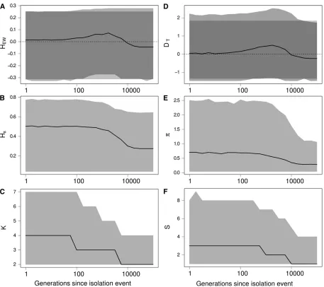
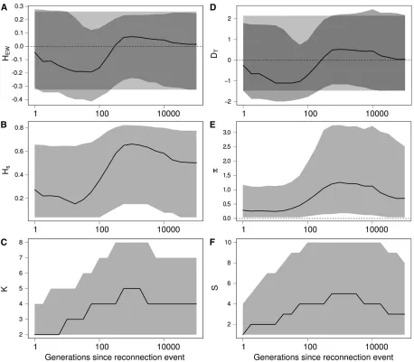
We followed the dynamics of the statistics and estimated their distribution as a function of time. The results in Figure 5 show that an isolation event produces the same signature on the Ewens–Watterson statistics (Figure 5A) and Tajima’s
D (Figure 5D), as expected from a bottleneck event and from directional selection. Indeed, following an isolation event, genetic drift first causes the elimination of rare alleles and then eliminates more common alleles. Conse-quently, the number of alleles K decreases more quickly than genetic diversity Hs (Figure 5, B and C). Similarly,
the number of segregating sites S decreases faster than the number of pairwise differenciesp (Figure 5, E and F). Therefore,DTandHEWare skewed toward positive values,
as expected after a bottleneck or under the effect of direc-tional selection. Moreover, the statistics remain skewed for a long period of time (,10,000 generations in our simula-tions, see Figure 5).
Results in Figure 6 show that a reconnection event can successively produce the same signature as expected from a population expansion or from a bottleneck event onHEW
(Figure 6A) andDT(Figure 6, B and C). Indeed, following
a reconnection event, migrantsfirst create an excess of rare variants. The number of alleles K increases more quickly than the genetic diversity Hs (Figure 6, B and C), and the
number of segregating sitesSincreases faster than the num-ber of pairwise differences p (Figure 6, E and F), which skews HEW and DT toward negative values. Second, new
alleles brought by migrants increase in frequency, creating an excess of common variants. Consequently Hs increases
more thanK, andp increases more thanS, which skewsDT
andHEWtoward positive values.
Interestingly, the observed duration of the periods in which both statistics are skewed are similar to the expected duration of the dynamics of genetic diversity (from Equation 8). After an isolation event, we observe, in Figure 5, that all statistics reach their equilibrium value within10,000 gen-erations (4Ngenerations). This duration corresponds to the value of the time required to reach within-population ge-netic diversity equilibrium after an isolation event, t2 ’
12,000 generations (4.8N generations, estimated from Equation 8 witha= 5%). In this example, genetic drift is stronger than mutation (2m1/2N) and thus t22N.t2
corresponds to the duration of the period in which the def-icit of rare alleles skews the distribution of HEW and DT.
After a reconnection event, we observe (Figure 6) that
HEW and DT reach a “peak” within 600 generations
(0.24Ngenerations). This duration corresponds to the value of the duration of the transient dynamics following a recon-nection event, t2 ’ 540 generations (0.216N generations,
estimated from Equation 8 with a= 5%). In this example, migration is stronger than genetic drift and mutation (m
1/2Nandm m), and thus,t21/2m.t2corresponds to
the period during which the distribution ofHEWandDT is
skewed. Subsequently,HEW andDT reach their equilibrium
value in80,000 generations (32Ngenerations); this dura-tion corresponds to the time required to reach the genetic diversity equilibrium value after a reconnection event,t1’
75,000 generations (30Ngenerations, estimated from Equa-tion 8 with a= 5%). t1 corresponds to the period during
which the deficit of rare alleles is eliminated.
In conclusion, both an isolation and a reconnection event induce changes in the proportion of rare alleles, which skews the values ofHEWandDT, thus producing a signature
that cannot be differentiated from the signature of past de-mographic events or of selection.
Discussion
We documented a simple neutral mechanism, which creates long-term peaks of genetic diversity. This peak of genetic diversity appears shortly after an abrupt increase in migra-tion and is conserved for a long time. We also demonstrated that such genetic diversity peaks can occur for a large and plausible range of population sizes, migration rates, muta-tion rates, and numbers of populamuta-tions. Subsequent to the genetic diversity peak, the rate of decay of genetic diversity was slow. Consequently, the mechanisms described here leave a strong and long-term footprint on genetic diversity that affects the Ewens–Watterson statistics and Tajima’s D
that are commonly used to infer the history of populations from genetic data.
(because of small migration or nonequilibrium genetic di-versity), we show that a genetic diversity peak is still ob-served (seeFile S3).
A connection event that occurs after an isolation period might play an important role on species diversification. Indeed, we have demonstrated that such events create an excess of genetic diversity. A high level of genetic diversity has often been hypothesized as being a key factor for species diversification. First, evolution from standing genetic varia-tion might be stronger than fromde novomutation (Gibson and Dworkin 2004; Hermisson and Pennings 2005; Myles
et al.2005; Barrett and Schluter 2008). Second, both theo-retical (Gavrilets 2003; Gavrilets and Losos 2009) and
em-pirical work suggest that a high level of preexisting genetic diversity in a population increases its rate of diversification (Harmonet al.2003; Seehausen 2004; Barrett and Schluter 2008). Interestingly, in several cases of adaptive radiation, a high genetic diversity of founder populations has been documented (e.g., Barrieret al.1999; Bezaultet al.2011). Several authors argued that the connection of populations after a period of isolation might have played an important role in many adaptive radiations (Hughes and Eastwood 2006; Antonelli and Sanmartín 2011; Bezault et al. 2011; Joyceet al.2011). Therefore, species that experienced pop-ulation isolation followed by reconnection events could have benefited from a temporary genetic diversity peak, which
Figure 5 Effect of an isolation event on Ewens–Watterson and Tajima’sDneutrality tests and on related summary statistics. (A) Ewens–Watterson statistics (HEW), (B) genetic diversity (Hs), (C) number of alleles (K), (D) Tajima’sD(DT), (E) number of pairwise differences (p), and (F) number of
segregating sites (S). For each statistics, the solid line represents the median of the distribution and the light shading represents the 97.5 and 2.5% quantiles of the distribution as a function of the number of generationstafter the isolation event. Dark shading in A and D represent the expected distribution of the statistics in an isolated population at equilibrium. Values ofHEWandDafter an isolation event are skewed toward positive values
has promoted the diversification of that species. Numerous species are known to have experienced such connectivity changes in the past and show remarkable levels of genetic and species diversity (Arnegard et al.1999). For example, cichlidfishes in the great African lakes experienced periods of habitat fragmentation and reconnection due to lake water levelfluctuations (Arnegardet al.1999); there is some ev-idence that these processes might have played a role in the explosive radiation of the species (Owenet al.1990; Young
et al.2009). Additionally, a high rate of speciation is corre-lated with the timeframe surrounding the uplift of the Northern Andes (Sedano and Burns 2010). The mechanisms
described here are thus expected to considerably affect the ability of species to adapt to novel environmental conditions and to diversify over a very long period of time.
Statistics on allelic frequencies such as the Ewens–Watterson statistics (Watterson 1978) and Tajima’s D (Tajima 1989) allow the inference of either selection or population dem-ographic changes. Here, we demonstrate that migration changes can lead to signatures that cannot be differentiated from a selection process or a population size change when using the Ewens–Watterson test and Tajima’sD. Therefore, past migration changes must be considered more carefully and should be viewed as an alternative explanation of bias
Figure 6 Effect of a reconnection event on Ewens–Watterson and Tajima’s D neutrality tests and on related summary statistics. (A) Ewens–Watterson statistics (HEW), (B) genetic diversity (Hs), (C) number of alleles (K), (D) Tajima’s D (DT), (E) number of pairwise differences (p), and (F) number of
segregating sites (S). For each statistics, the solid line represents the median of the distribution, and the light shading represents the 97.5% and 2.5% quantiles of the distribution, as a function of the number of generationstafter the isolation event. Dark shading in A and D represent the expected distribution of the statistics in an isolated equilibrium population. Values ofHEWandDafter a reconnection event arefirst skewed toward negative
values (signature of a population expansion or balancing selection) and then toward positive values (signature of a bottleneck or directional selection), while there was no change in the size of the population.KandSfirst increase more quickly thanHsandpbecause immigrants bring rare alleles, and
thenHsandpreach a higher value because immigrant alleles increase in frequency. Finally, alleles are eliminated by genetic drift until the statistics reach
their expected equilibrium value when populations are connected. Coalescence simulations of a 1 kb locus with a mutation rate of 2·1028per bp,
in neutrality tests and bottleneck or expansion signals. Re-cently, authors have shown that population structure can bias neutrality tests and produce false bottleneck signals (Leblois
et al.2006; Städler et al.2009; Chikhi et al.2010) and that shortly after an isolation event departure from the neutrality can be incorrectly inferred (as shown with simulations by Broquet et al. 2010 and discussed in Waples 2010). The proper interpretation of genetic signatures is crucial for the understanding of the evolutionary history of populations. An interesting extension of this work would be to analyze in more detail the molecular signature of the mechanisms described here and to provide methods that allow the differentiation of such events from selection or demographic changes. More-over, our results are also relevant for the study of genealogies. Indeed, genetic identities as considered here are commonly used to describe coalescence time distributions (Slatkin 1991; Rousset 1996; Wakeley 1999). Future investigations should also investigate the consequences of isolation and connection events on phylogenetic tree reconstruction. Statistical tools that are available to estimate demographic parameters clas-sically focus on a priori specific scenarios (e.g., population bottleneck, expansion, population with constant migration, population split with subsequent migration; see review in Kuh-ner 2009). Given the strong impact of migration changes on genetic diversity, accounting for such scenarios is necessary. Recent methods allowing a larger range of population demo-graphic scenarios, such as approximate Bayesian computation (Beaumont et al. 2002; Beaumont 2010), may be powerful tools with which to disentangle the signature of demographic processes from the observed genetic diversity.
One of the major goals of conservation genetics is to maintain genetic diversity, decrease extinction risks, avoid inbreeding depression, maintain species evolutionary poten-tial, and decrease species vulnerability to environmental change (Gilpin and Soule 1986; Newman and Pilson 1997; Jumpet al.2009). In this context, conservationists need to estimate the genetic diversity of a population and its effec-tive size. Such measures are commonly obtained from ge-netic data and are estimated with standard statistics (Wright 1950; Jorde and Ryman 2007). Although new approaches that consider populations at a nonequilibrium state are emerging, to estimate population size changes and instanta-neous migration rates (e.g., Hey and Nielsen 2004), the expected level of genetic diversity is still commonly esti-mated assuming that populations are at an equilibrium. As shown here, genetic diversity is more likely to be in a transient state. We have demonstrated that reconnecting isolated pop-ulations increases genetic diversity above the expected equi-librium value, while isolating populations induces a slow decrease of genetic diversity. Consequently, any estimate inferred from data collected from a population that under-went strong migration changes will not reflect the demo-graphic situation of the population (e.g., census size, genetic diversity). This can have drastic consequences on the selec-tion of conservaselec-tion strategies and for the management of species (Pearse and Crandall 2004; Caballeroet al.2010).
Acknowledgments
The authors thank two anonymous reviewers and Noah Rosenberg for their valuable comments and suggestions, which increased the clarity and the scope of the article. This project was funded by the Swiss National Research Founda-tion (SNRF) grant nos. PZ00P3–121702, PZ00P3–139421/1, and 31003A–130065.
Literature Cited
Antonelli, A., and I. Sanmartín, 2011 Why are there so many plant species in the neotropics? Taxon 60: 403–414.
Antonelli, A., J. A. A. Nylander, C. Persson, and I. Sanmartín, 2009 Tracing the impact of the andean uplift on neotropical plant evolution. Proc. Natl. Acad. Sci. USA 106: 9749–9754. Arnegard, M. E., J. A. Markert, P. D. Danley, J. R. Stauffer, A. J.
Ambaliet al., 1999 Population structure and colour variation of the cichlid fishes labeotropheus fuelleborni ahl along a re-cently formed archipelago of rocky habitat patches in southern Lake Malawi. Proc. R. Soc. Lond. B Biol. Sci. 266: 119–130. Barrett, R. D. H., and D. Schluter, 2008 Adaptation from standing
genetic variation. Trends Ecol. Evol. 23: 38–44.
Barrier, M., B. G. Baldwin, R. H. Robichaux, and M. D. Purugganan, 1999 Interspecific hybrid ancestry of a plant adaptive radia-tion: allopolyploidy of the Hawaiian silversword alliance (Aster-aceae) inferred from floral homeotic gene duplications. Mol. Biol. Evol. 16: 1105–1113.
Beaumont, M. A., 2010 Approximate Bayesian computation in evolution and ecology. Annu. Rev. Ecol. Evol. Syst. 41: 379–406. Beaumont, M. A., W. Zhang, and D. J. Balding, 2002 Approximate Bayesian computation in population genetics. Genetics 162: 2025–2035.
Bezault, E., S. Mwaiko, and O. Seehausen, 2011 Population ge-nomic tests of models of adaptive radiation in Lake Victoria re-gion Cichlidfish. Evolution 65: 3381–3397.
Broquet, T., S. Angelone, J. Jaquiery, P. Joly, J.-P. Lena et al., 2010 Genetic bottlenecks driven by population disconnection. Conserv. Biol. 24: 1596–1605.
Caballero, A., S. T. Rodriguez-Ramilo, V. Avila, and J. Fernandez, 2010 Management of genetic diversity of subdivided popula-tions in conservation programmes. Conserv. Genet. 11: 409–419. Chikhi, L., V. C. Sousa, P. Luisi, B. Goossens, and M. A. Beaumont, 2010 The confounding effects of population structure, genetic diversity and the sampling scheme on the detection and quan-tification of population size changes. Genetics 186: 983–995. Colosimo, P. F., K. E. Hosemann, S. Balabhadra, G. Villarreal, M.
Dicksonet al., 2005 Widespread parallel evolution in stickle-backs by repeatedfixation of ectodysplasin alleles. Science 307: 1928–1933.
Cook, L. M., 2008 Species richness in Madeiran land snails, and its causes. J. Biogeogr. 35: 647–653.
Delaney, K. S., S. P. D. Riley, and R. N. Fisher, 2010 A rapid, strong, and convergent genetic response to urban habitat frag-mentation in four divergent and widespread vertebrates. PLoS ONE 5: e12767.
Domingues, V. S., Y.-P. Poh, B. K. Peterson, P. S. Pennings, J. D. Jensen
et al. 2012 Evidence of adaptation from ancestral variation in young populations of beach mice. Evolution 66: 3209–3223. Ewens, W. J., 1972 The sampling theory of selectively neutral
alleles. Theor. Popul. Biol. 3: 87–112.
Excoffier, L., and H. E. L. Lischer, 2010 Arlequin suite ver 3.5: a new series of programs to perform population genetics anal-yses under linux and windows. Mol. Ecol. Res. 10: 564–567. Excoffier, L., M. Foll, and R. J. Petit, 2009 Genetic consequences
of range expansions. Annu. Rev. Ecol. Evol. Syst. 40: 481–501. Falush, D., M. Stephens, and J. K. Pritchard, 2003 Inference of population structure using multilocus genotype data: linked loci and correlated allele frequencies. Genetics 164: 1567–1587. Fay, J. C., and C. I. Wu, 2000 Hitchhiking under positive
darwin-ian selection. Genetics 155: 1405–1413.
Feder, J. L., S. H. Berlocher, J. B. Roethele, H. Dambroski, J. J. Smith et al., 2003 Allopatric genetic origins for sympatric host-plant shifts and race formation in rhagoletis. Proc. Natl. Acad. Sci. USA 100: 10314–10319.
Fisher, R. A., 1922 Darwinian evolution of mutations. Eugen. Rev. 14: 31–34.
Fisher, R. A., 1930 The Genetical Theory of Natural Selection. Clar-endon Press, Oxford.
Frankham, R., 1995 Conservation genetics. Annu. Rev. Genet. 29: 305–327.
Fu, Y. X., and W. H. Li, 1993 Statistical tests of neutrality of mutations. Genetics 133: 693–709.
Galis, F., and J. A. Metz, 1998 Why are there so many cichlid species? Trends Ecol. Evol. 13: 1–2.
Gavrilets, S., 2003 Perspective: models of speciation: What have we learned in 40 years? Evolution 57: 2197–2215.
Gavrilets, S., and J. B. Losos, 2009 Adaptive radiation: contrasting theory with data. Science 323: 732–737.
Gibson, G., and I. Dworkin, 2004 Uncovering cryptic genetic var-iation. Nat. Rev. Genet. 5: 681–690.
Gilpin, M., and M. Soule, 1986 Minimum viable populations: pro-cesses of species extinction, pp. 19–34 in Conservation Biology: The Science of Scarcity and Diversity. Sinauer, Sunderland, MA. Gravel, S., 2012 Population genetics models of local ancestry.
Genetics 191: 607–619.
Green, R. E., J. Krause, A. W. Briggs, T. Maricic, U. Stenzelet al., 2010 A draft sequence of the neandertal genome. Science 328: 710–722. Harmon, L. J., J. A. Schulte, A. Larson, and J. B. Losos, 2003 Tempo
and mode of evolutionary radiation in iguanian lizards. Science 301: 961–964.
Hedrick, P. W., and S. T. Kalinowski, 2000 Inbreeding depression in conservation biology. Annu. Rev. Ecol. Syst. 31: 139–162. Hermisson, J., and P. S. Pennings, 2005 Soft sweeps: molecular
population genetics of adaptation from standing genetic varia-tion. Genetics 169: 2335–2352.
Hernandez, R. D., J. L. Kelley, E. Elyashiv, S. C. Melton, A. Auton
et al., 2011 Classic selective sweeps were rare in recent human evolution. Science 331: 920–924.
Hewitt, G., 2000 The genetic legacy of the quaternary ice ages. Nature 405: 907–913.
Hewitt, G. M., 2004 Genetic consequences of climatic oscillations in the quaternary. Philos. Trans. R. Soc. Lond. B Biol. Sci. 359: 183–195, discussion 195.
Hey, J., and R. Nielsen, 2004 Multilocus methods for estimating population sizes, migration rates and divergence time, with ap-plications to the divergence ofDrosophila pseudoobscuraandD. persimilis. Genetics 167: 747–760.
Hughes, C., and R. Eastwood, 2006 Island radiation on a conti-nental scale: exceptional rates of plant diversification after uplift of the andes. Proc. Natl. Acad. Sci. USA 103: 10334–10339. Jensen, J. D., Y. Kim, V. B. DuMont, C. F. Aquadro, and C. D.
Bustamante, 2005 Distinguishing between selective sweeps and demography using dna polymorphism data. Genetics 170: 1401–1410.
Jimenez, J. A., K. A. Hughes, G. Alaks, L. Graham, and R. C. Lacy, 1994 An experimental study of inbreeding depression in a nat-ural habitat. Science 266: 271–273.
Jones, F. C., M. G. Grabherr, Y. F. Chan, P. Russell, E. Mauceliet al., 2012 The genomic basis of adaptive evolution in threespine sticklebacks. Nature 484: 55–61.
Jorde, P. E., and N. Ryman, 2007 Unbiased estimator for genetic drift and effective population size. Genetics 177: 927–935. Joyce, D. A., D. H. Lunt, M. J. Genner, G. F. Turner, R. Billset al.,
2011 Repeated colonization and hybridization in Lake Malawi cichlids. Curr. Biol. 21: R108–R109.
Jump, A. S., R. Marchant, and J. Peñuelas, 2009 Environmental change and the option value of genetic diversity. Trends Plant Sci. 14: 51–58.
Karlin, S., 1982 Classifications of selection migration structures and conditions for a protected polymorphism. Evol. Biol. 14: 61–204.
Keller, I., W. Nentwig, and C. R. Largiader, 2004 Recent habitat fragmentation due to roads can lead to significant genetic dif-ferentiation in an abundantflightless ground beetle. Mol. Ecol. 13: 2983–2994.
Kim, Y., and D. Gulisija, 2010 Signatures of recent directional selection under different models of population expansion during colonization of new selective environments. Genetics 184: 571– 585.
Kim, Y., and R. Nielsen, 2004 Linkage disequilibrium as a signa-ture of selective sweeps. Genetics 167: 1513–1524.
Kim, Y., and W. Stephan, 2002 Detecting a local signature of genetic hitchhiking along a recombining chromosome. Genetics 160: 765–777.
Kimura, M., and J. F. Crow, 1964 The number of alleles that can be maintained in afinite population. Genetics 49: 725–738. Kreitman, M., 2000 Methods to detect selection in populations
with applications to the human. Annu. Rev. Genomics Hum. Genet. 1: 539–559.
Kuhner, M. K., 2009 Coalescent genealogy samplers: windows in-to population hisin-tory. Trends Ecol. Evol. 24: 86–93.
Lambeck, K., F. Antonioli, A. Purcell, and S. Silenzi, 2004 Sea-level change along the Italian coast for the past 10,000 yr. Quat. Sci. Rev. 23: 1567–1598.
Latter, B. D., 1973 The island model of population differentiation: a general solution. Genetics 73: 147–157.
Leblois, R., A. Estoup, and R. Streiff, 2006 Genetics of recent habitat contraction and reduction in population size: Does iso-lation by distance matter? Mol. Ecol. 15: 3601–3615.
Li, H., and W. Stephan, 2006 Inferring the demographic history and rate of adaptive substitution in Drosophila. PLoS Genet. 2: e166.
Maruyama, T., 1970 Effective number of alleles in a subdivided population. Theor. Popul. Biol. 1: 273–306.
Miller, J., and R. Hobbs, 2002 Conservation where people live and work. Conserv. Biol. 16: 330–337.
Myles, S., N. Bouzekri, E. Haverfield, M. Cherkaoui, J.-M. Dugoujon
et al., 2005 Genetic evidence in support of a shared Eurasian– North African dairying origin. Hum. Genet. 117: 34–42. Nagylaki, T., 1974 The decay of genetic variability in
geographi-cally structured populations. Proc. Natl. Acad. Sci. USA 71: 2932–2936.
Nagylaki, T., 1977 Decay of genetic variability in geographically structured populations. Proc. Natl. Acad. Sci. USA 74: 2523– 2525.
Nagylaki, T., 1979 The island model with stochastic migration. Genetics 91: 163–176.
Nei, M., 1973 Analysis of gene diversity in subdivided popula-tions. Proc. Natl. Acad. Sci. USA 70: 3321–3323.
Nei, M., and M. W. Feldman, 1972 Identity of genes by descent within and between populations under mutation and migration pressures. Theor. Popul. Biol. 3: 460–465.
Newman, D., and D. Pilson, 1997 Increased probability of extinc-tion due to decreased genetic effective populaextinc-tion size: experi-mental populations of Clarkia pulchella. Evolution 51: 354–362. Nielsen, R., 2005 Molecular signatures of natural selection. Annu.
Rev. Genet. 39: 197–218.
Nielsen, R., C. Bustamante, A. G. Clark, S. Glanowski, T. B. Sackton
et al., 2005 A scan for positively selected genes in the genomes of humans and chimpanzees. PLoS Biol. 3: e170.
Noel, S., M. Ouellet, P. Galois, and F.-J. Lapointe, 2007 Impact of urban fragmentation on the genetic structure of the eastern red-backed salamander. Conserv. Genet. 8: 599–606.
Orr, H. A., and A. J. Betancourt, 2001 Haldane’s sieve and adapta-tion from the standing genetic variaadapta-tion. Genetics 157: 875–884. Owen, R. B., R. Crossley, T. C. Johnson, D. Tweddle, I. Kornfield
et al., 1990 Major low levels of Lake Malawi and their impli-cations for speciation rates in cichlidfishes. Proc. R. Soc. Lond. B Biol. Sci. 240: 519–553.
Pavlidis, P., J. D. Jensen, and W. Stephan, 2010 Searching for footprints of positive selection in whole-genome snp data from nonequilibrium populations. Genetics 185: 907–922.
Pearse, D. E., and K. A. Crandall, 2004 Beyond fst: analysis of population genetic data for conservation. Conserv. Genet. 5: 585–602 .10.1007/s10592–004–1863-z.
Pelz, H.-J., S. Rost, M. Hünerberg, A. Fregin, A.-C. Heiberget al., 2005 The genetic basis of resistance to anticoagulants in ro-dents. Genetics 170: 1839–1847.
Peter, B. M., D. Wegmann, and L. Excoffier, 2010 Distinguishing between population bottleneck and population subdivision by a Bayesian model choice procedure. Mol. Ecol. 19: 4648–4660. Price, A. L., A. Tandon, N. Patterson, K. C. Barnes, N. Rafaelset al., 2009 Sensitive detection of chromosomal segments of distinct ancestry in admixed populations. PLoS Genet. 5: e1000519. Pritchard, J. K., M. Stephens, and P. Donnelly, 2000 Inference of
population structure using multilocus genotype data. Genetics 155: 945–959.
Rice, S. H., and A. Papadopoulos, 2009 Evolution with stochastic
fitness and stochastic migration. PLoS ONE 4: e7130.
Rousset, F., 1996 Equilibrium values of measures of population sub-division for stepwise mutation processes. Genetics 142: 1357–1362. Schluter, D., E. A. Clifford, M. Nemethy, and J. S. McKinnon, 2004 Parallel evolution and inheritance of quantitative traits. Am. Nat. 163: 809–822.
Sedano, R. E., and K. J. Burns, 2010 Are the Northern Andes a species pump for neotropical birds?: Phylogenetics and bio-geography of a clade of neotropical tanagers (aves: Thraupini). J. Biogeogr. 37: 325–343.
Seehausen, O., 2004 Hybridization and adaptive radiation. Trends Ecol. Evol. 19: 198–207.
Shpak, M., J. Wakeley, D. Garrigan, and R. C. Lewontin, 2010 A structured coalescent process for seasonallyfluctuating popula-tions. Evolution 64: 1395–1409.
Slatkin, M., 1991 Inbreeding coefficients and coalescence times. Genet. Res. 58: 167–175.
Smith, J. M., 1970 Population size, polymorphism, and the rate of non-Darwinian evolution. Am. Nat. 104: 231–237.
Städler, T., B. Haubold, C. Merino, W. Stephan, and P. Pfaffelhuber, 2009 The impact of sampling schemes on the site frequency spectrum in nonequilibrium subdivided populations. Genetics 182: 205–216.
Sturmbauer, C., S. Baric, W. Salzburger, L. Rüber, and E. Verheyen, 2001 Lake levelfluctuations synchronize genetic divergences of cichlidfishes in African lakes. Mol. Biol. Evol. 18: 144–154. Tajima, F., 1983 Evolutionary relationship of DNA sequences in
finite populations. Genetics 105: 437–460.
Tajima, F., 1989 Statistical method for testing the neutral muta-tion hypothesis by DNA polymorphism. Genetics 123: 585–595. Takahata, N., and M. Nei, 1985 Gene genealogy and variance of interpopulational nucleotide differences. Genetics 110: 325– 344.
Turner, R. C., J. C. Levy, and A. Clark, 1993 Complex genetics of type 2 diabetes: thrifty genes and previously neutral polymor-phisms. Q. J. Med. 86: 413–417.
Vandergast, A. G., E. A. Lewallen, J. Deas, A. J. Bohonak, D. B. Weissmanet al., 2009 Loss of genetic connectivity and diver-sity in urban microreserves in a southern California endemic Jerusalem cricket (Orthoptera: Stenopelmatidae: Stenopelma-tus n. sp‘‘santa monica’’). J. Insect Conserv. 13: 329–345. Wakeley, J., 1999 Nonequilibrium migration in human history.
Genetics 153: 1863–1871.
Waples, R. S., 2010 Spatial-temporal stratifications in natural populations and how they affect understanding and estimation of effective population size. Mol Ecol Resour 10: 785–796. Watterson, G. A., 1978 The homozygosity test of neutrality.
Ge-netics 88: 405–417.
Whitlock, M. C., 1992 Temporalfluctuations in demographic pa-rameters and the genetic variance among populations. Evolu-tion 46: 608–615.
Whitlock, M. C., and N. H. Barton, 1997 The effective size of a subdivided population. Genetics 146: 427–441.
Wright, S., 1931 Evolution in Mendelian populations. Genetics 16: 97–159.
Wright, S., 1950 Genetical structure of populations. Nature 166: 247–249.
Young, K. A., J. M. Whitman, and G. F. Turner, 2009 Secondary contact during adaptive radiation: a community matrix for Lake Malawi cichlids. J. Evol. Biol. 22: 882–889.
Zhang, H., J. Yan, G. Zhang, and K. Zhou, 2008 Phylogeography and demographic history of Chinese black-spotted frog popula-tions (Pelophylax nigromaculata): evidence for independent re-fugia expansion and secondary contact. BMC Evol. Biol. 8: 21.
Appendix A: Dynamics of Genetic Diversity
In this appendix, we describe the temporal change of genetic diversity (derivation of Equations 4a and 8 and the separation of the dynamics of genetic diversity into two timescales).
Temporal change of genetic diversity
The solution to Equation 3 is
Ft ¼AtðF02FeqÞ þFeq: (A1)
Denoting Pthe transformation matrix with eigenvectorU1(associated withl1) asfirst column and eigenvectorU2
(asso-ciated withl2) as second column,
P¼ ðU1 U2Þ (A2)
and denoting
y10
y20
¼P21ðF
02FeqÞ; (A3)
Equation A1 becomes
Ft¼P
l1 0
0 l2
t
P21ðF
02FeqÞ þFeq
¼P
l1 0
0 l2
t
y10
y20
þFeq
¼y10U1lt1þy20U2lt2þFeq:
(A4)
Further, denotingC1=y10U1andC2=y20U2leads to Equation 4a.
Ftchanges according to two exponential decay functions,lt1andl t
2. Their rates of change aredl t
1=dt¼lnðl1Þ·elnðl1Þtand dlt2=dt¼lnðl2Þ·e
lnðl2Þt, respectively. Thusr
1= ln(l1) andr2= ln(l2) are the decay constants that determine the rate of
change of functionslt
1 andl
t 2.
Therefore, the eigenvalues of matrixAcan be used to compute the rates of change of genetic diversity. Asl1.l2and both eigenvalues are,1, we have |r2|.|r1|, and thusC2lt2tends to 0 faster thanC1lt1.r2determines the transient rate of
change of genetic diversity, whiler1determines the asymptotic rate of change of genetic diversity.
We now want to simplify the expression of the rates of change of genetic diversity. To do so, we can rewrite Equation 5 as
l1¼ð12mÞ 2
2 "
að12cÞ þ12bþ ð12að12cÞ þbÞ
ffiffiffiffiffiffiffiffiffiffiffiffiffiffiffiffiffiffiffiffiffiffiffiffiffiffiffiffiffiffiffiffiffiffiffiffiffiffiffiffiffiffiffiffi 12 4bc
ð12að12cÞ þbÞ2
s #
l2¼ð12mÞ 2
2 "
að12cÞ þ12b2ð12að12cÞ þbÞ
ffiffiffiffiffiffiffiffiffiffiffiffiffiffiffiffiffiffiffiffiffiffiffiffiffiffiffiffiffiffiffiffiffiffiffiffiffiffiffiffiffiffiffiffi 12 4bc
ð12að12cÞ þbÞ2
s #
:
With 4bc(12a(12c) +b)2(asm1 andN1), and given thatpffiffiffiffiffiffiffiffiffiffiffi12x¼121
2xþoðxÞ, Equation 5 further simplifies
to
l1¼ ð12mÞ2
12 bc 12að12cÞ þb
l2¼ ð12mÞ2
að12cÞ2bþ bc
12að12cÞ þb
:
Considering that migration rates and mutation rates are small, we can neglect terms inm2, 1=N2,m2,m/N,mm,andm=N,
l1¼122m21=
2nN
1þn21
nM
l2¼122m22m
n n212
1 2Nþ1=
2nN
1þn21
nM
(A5)
and thus
r1¼ln
122m21=
2nN
1þn21
nM
r2¼ln
122m22m n n212
1 2Nþ1=
2nN
1þn21
nM
:
(A6)
Assuming that migration and mutation rates are small, and that local population sizes are large (N 1), Equation A6 simplifies to Equation 6 as ln(12x) =2x+o(x).
Respective length of the asymptotic and transient dynamics periods
We denotet1andt2as the times needed forlt1 andl t
2 to be reduced to a valuea, wherea2]0; 1],
lt1
1 ¼a
lt2
2 ¼a;
(A7)
which leads to
t1¼lnðaÞ
r1
t2¼lnðaÞ
r2 :
(A8)
Assuming small migration and mutation rates and large local population sizes, we can replace the expressions ofr1andr2
from Equation 6 into Equation A8, and we obtain Equation 8.Ftapproximately follows
Ft ’
8 < :
FeqþC
1lt1þC2lt2 fort,t2
FeqþC
1lt1 fort2,t,t1
Feq fort
1,t:
(A9)
Timescales separation
This section presents the conditions fort1t2. Whent1t2,lt22’0 andl t2
1 ’1; thus, Equation A9 simplifies to
Ft’
8 < :
FeqþC
1þC2lt2 for t,t2
FeqþC
1lt1 for t2,t,t1
Feq for t
1,t:
(A10)
Equation A10 decomposes the dynamics ofFtinto two timescales: atransient periodof lengtht2and anasymptotic period
of lengtht12t2’t1. Fort.t1, the genetic identity is close to its equilibrium valueFeq, sot1can be interpreted as the
duration of the disequilibrium period.
Equation A10 is true if atexists such thatlt1 ’1 andl t
2 ’0. For simplicity, we consider thatl t
1 ’1 ifl
t
1 $0:95 and
thatlt2 ’0 ifl t
2 #0:05. Thus, Equation A10 is a good approximation if atexists such that
lt
1$0:95
lt
2#0:05
⇒ 8 > < > :
t#lnð0:95Þ
lnðl1Þ
lt
2#0:05:
(A11)
llnð0:95Þ=lnðl1Þ
2 #0:05 (A12)
demonstrates that fort¼lnð0:95Þ=lnðl1Þ, we havelt
1 $0:95 andlt2 #0:05. This provides a sufficient proof of proposition
(A11).
We can demonstrate that proposition (A12) depends only on the ratiot1=t2 ¼lnðl2Þ=lnðl1Þ(see definitions oft1andt2
Equation 7). Proposition (A12) leads to
llnð0:95Þ=lnðl1Þ
2 #0:05
⇔elnð0:95Þ½lnðl2Þ=lnðl1Þ#0:05
⇔lnð0:95Þt1
t2#lnð0:05Þ
⇔t1
t2$
lnð0:05Þ lnð0:95Þ:
Therefore, the conditiont1=t2$lnð0:05Þ=lnð0:95Þis necessary and sufficient to prove propositions (A12) and (A11) and the
validity of Equation A10. As lnð0:05Þ=lnð0:95Þ ’58:4, Equation A10 is valid whent1=t2.58:4. Considering thatmandm
are small, and that Nis large, this ratio is approximately equal to (from Equation 8)
t1
t2’
2mþ2mðn=½n21Þ þ ð1=2NÞ2ð1=2NeÞ
2mþ ð1=2NeÞ :
(A13)
From Equation A13 we can derive the conditions of the timescales separation of the dynamics of genetic diversity (i.e., the parameter values for whicht1t2). Whenn.14, differences are the highest (t1t2), in the domain wherem1=2Nand
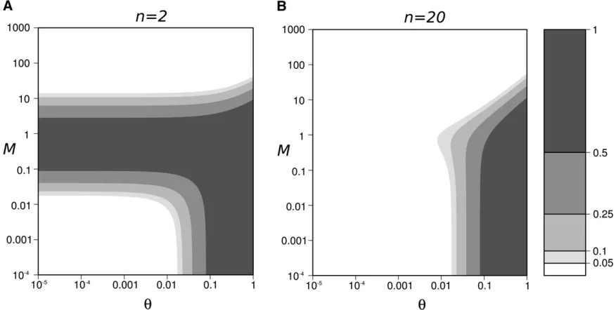
also whenm1=2Nandm.m. Whenn#14, the same conditions apply fort1t2except in a restricted domain where m’1=2N (m ðn21Þ=2nN or m ðn21Þ=2nN are required for t1 t2; see Figure A1). Indeed, denoting A¼lnð0:05Þ=lnð0:95Þ,t1=t2.Aimplies that
M.Aþ122nþ ðA21Þnuþ
ffiffiffiffi
D
p
2ðn2=ðn21ÞÞ or M,
Aþ122nþ ðA21Þnu2pffiffiffiffiD
2ðn2=ðn21ÞÞ ; (A14a)
where
D¼ ðAþ1ÞðAþ124nÞ þ2nuA221þn2ðA21Þ2u2: (A14b)
Foru1, we can neglect terms that do not containu, and conditions (A14) simplify to
M.ðA21Þn21
n u; (A15)
which simplifies toMu.
Foru1, terms that containucan be neglected in Equation A14, which yields the following conditions:
M.Aþ122nþ
ffiffiffiffiffiffiffiffiffiffiffiffiffiffiffiffiffiffiffiffiffiffiffiffiffiffiffiffiffiffiffiffiffiffiffiffiffiffiffiffiffiffi ðAþ1ÞðAþ124nÞ
p
2ðn2=ðn21ÞÞ or M,
Aþ122n2pðffiffiffiffiffiffiffiffiffiffiffiffiffiffiffiffiffiffiffiffiffiffiffiffiffiffiffiffiffiffiffiffiffiffiffiffiffiffiffiffiffiffiAþ1ÞðAþ124nÞ
2ðn2=ðn21ÞÞ (A16)
Therefore, Equation A10 is not valid when conditions of Equation A16 are not met. This domain is centered around
M¼ ððn21Þ=nÞ, as
Aþ122nþpðffiffiffiffiffiffiffiffiffiffiffiffiffiffiffiffiffiffiffiffiffiffiffiffiffiffiffiffiffiffiffiffiffiffiffiffiffiffiffiffiffiffiAþ1ÞðAþ124nÞ
2ðn2=ðn21ÞÞ and
Aþ122nþpðffiffiffiffiffiffiffiffiffiffiffiffiffiffiffiffiffiffiffiffiffiffiffiffiffiffiffiffiffiffiffiffiffiffiffiffiffiffiffiffiffiffiAþ1ÞðAþ124nÞ
2ðn2=ðn21ÞÞ
equalize toM¼ ððn21Þ=nÞ, forA= 4n21. The size of this domain decreases whennincreases (Figure A1), and Equation A10 is valid for any value ofMin the domainu1 whenn.14 (as conditions (A16) are relaxed when 4n.A+ 1, with
Appendix B: Peak of Genetic Diversity Generated by a Reconnection Event
We derive first the value of the peak of within-population genetic diversity, DHs, and the transient excess of
between-population genetic diversity, DHb, generated by a reconnection event. Second, we characterize their dependency on the
migration rate, mutation rate, size, and number of populations.
Derivation ofDH
We denote the vector of genetic diversity excess at the end of the transient dynamics phase asDH¼
ð
DHs DHbÞ
. The genetic diversity at the end of the transient dynamics phase is approximatelyHt2 ¼12ðFeqþC1lt2
1Þ(from Equation A9
whent’t2). ThusDHis approximately
DH¼Ht22H
eq
¼12FeqþC 1lt12
2ð12FeqÞ
¼ 2C1lt12:
(B1)
The peak of genetic diversity depends onC1=y10U1(from Equations A2 and A3). To derive the value ofC1, we computeU1
andy10. The eigenvectorU1¼
ð
u11u21
Þ
is associated withl1and followsAU1¼l1U1: (B2)
Equation B2 leads to the condition thatu21¼ 2ððað12cÞ2ð12bÞ2
ffiffiffiffiffiffiffiffiffi
Dred
p
Þ=2ð12aÞÞu11, whereDred= (12a(12c) + b)224bc. We setu
11= 2(12a), leading to
U1¼
2ð12aÞ
12að12cÞ2bþ
ffiffiffiffiffiffiffiffiffiffiffiffiffiffiffiffiffiffiffiffiffiffiffiffiffiffiffiffiffiffiffiffiffiffiffiffiffiffiffiffiffiffiffiffiffiffiffiffiffi ð12að12cÞ þbÞ224bc
q !:
Similarly, we can determine the eigenvector associated withl2:
U2¼
2ð12aÞ
12að12cÞ2b2
ffiffiffiffiffiffiffiffiffiffiffiffiffiffiffiffiffiffiffiffiffiffiffiffiffiffiffiffiffiffiffiffiffiffiffiffiffiffiffiffiffiffiffiffiffiffiffiffiffi ð12að12cÞ þbÞ224bc
q !:
Denoting the initial value of genetic identityF0¼
ð
Fs;0Fb;0
Þ
and replacing the expression ofU1andU2in Equation A3 leads toFigure A1 Domain of validity of Equation A10 (white contours), as a function of the strength of migration (M) and mutation (u), (A)n= 2, (B)n= 20. The dark shading represent the domains where the validity of Equation A10 is poor (i.e., the exact value ofllnð0:95Þ=lnðl1Þ