Asexual but Not Clonal: Evolutionary Processes in Automictic Populations

| INVESTIGATION

Asexual but Not Clonal: Evolutionary Processes in

Automictic Populations

Jan Engelstädter1 School of Biological Sciences, The University of Queensland, Brisbane, 4072, Australia ORCID ID: 0000-0003-3340-918X (J.E.)

ABSTRACT Many parthenogenetically reproducing animals produce offspring not clonally but through different mechanisms collectively referred to as automixis. Here, meiosis proceeds normally but is followed by a fusion of meiotic products that restores diploidy. This mechanism typically leads to a reduction in heterozygosity among the offspring compared to the mother. Following a derivation of the rate at which heterozygosity is lost at one and two loci, depending on the number of crossovers between loci and centromere, a number of models are developed to gain a better understanding of basic evolutionary processes in automictic populations. Analytical results are obtained for the expected neutral genetic variation, effective population size, mutation–selection balance, selection with overdominance, the spread of beneficial mutations, and selection on crossover rates. These results are complemented by numerical investigations elucidating how associative overdominance (two off-phase deleterious mutations at linked loci behaving like an overdominant locus) can in some cases maintain heterozygosity for prolonged times, and how clonal interference affects adaptation in automictic populations. These results suggest that although automictic populations are expected to suffer from the lack of gene shuffling with other individuals, they are nevertheless, in some respects, superior to both clonal and outbreeding sexual populations in the way they respond to beneficial and deleterious mutations. Implications for related genetic systems such as intratetrad mating, clonal reproduction, selfing, as well as different forms of mixed sexual and automictic reproduction are discussed.

KEYWORDSautomixis; parthenogenesis; neutral genetic variation; overdominance; mutation–selection balance; central fusion

T

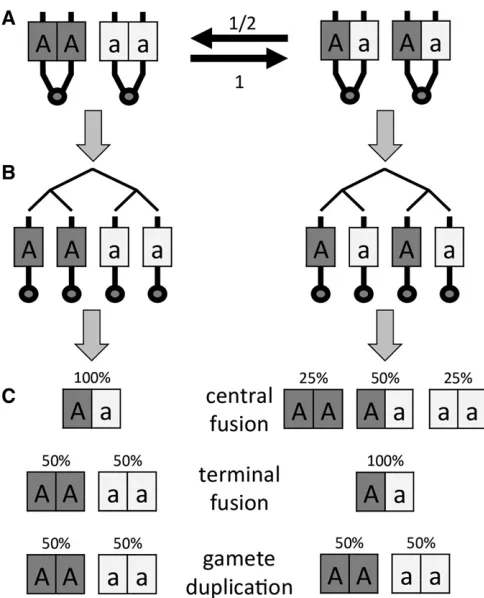
HE vast majority of animals and plants reproduce via the familiar mechanism of sex (Bell 1982): haploid gametes are produced through meiosis, and these fuse to form diploid offspring that are a genetic mix of their parents. Conversely, bacteria, many unicellular, and some multicellular eukary-otes reproduce clonally, i.e., their offspring are genetically identical to their mother. These two extreme genetic systems can also be alternated,e.g., a few generations of clonal re-production followed by one round of sexual rere-production. Such systems are found in many fungi (e.g., yeast) but also in animals such as aphids that exhibit“cyclical parthenogen-esis.”However, there are also genetic systems that resist an easy classification into“sexual”and“asexual.”Among them are automixis and related systems in which a modified meiosis

takes place in females, leading to offspring that develop from unfertilized but diploid eggs and that may be genetically di-verse and distinct from their mother (Suomalainen et al. 1987; Stenberg and Saura 2009). Explicably, there is much confusion and controversy about terminology in such sys-tems, with some authors referring to them as asexual (be-cause there is no genetic mixing between different lineages) and others as sexual (e.g., because they involve a form of meiosis and/or resemble selfing). Without entering this de-bate, I will adopt the former convention here, acknowledging that the latter is also valid and useful in some contexts. Also note that clonal,“ameiotic”reproduction in animals is usually referred to as apomixis but that this term has a different meaning in plants (Asker and Jerling 1992; van Dijk 2009). A good starting point for understanding automixis is to consider a specific system. One system that is particularly well studied is the South African honeybee subspeciesApis melli-fera capensis, the Cape honeybee (reviewed in Goudie and Oldroyd 2014). WithinA. mellifera capensis, workers can lay unfertilized eggs that develop parthenogenetically into dip-loid female offspring via a mechanism called“central fusion” Copyright © 2017 by the Genetics Society of America

doi:https://doi.org/10.1534/genetics.116.196873

Manuscript received October 17, 2016; accepted for publication March 21, 2017; published Early Online April 3, 2017.

Supplemental material is available online atwww.genetics.org/lookup/suppl/doi:10. 1534/genetics.116.196873/-/DC1.

1_{Address for correspondence: The University of Queensland, School of Biological}

(Verma and Ruttner 1983; Suomalainenet al.1987). Here, meiosis proceeds normally, producing four haploid nuclei, but diploidy is then restored through fusion of the egg pro-nucleus with the polar body separated in meiosis I. This means that in the absence of recombination between a given locus and its associated centromere, the maternal allelic state at this locus is restored and in particular, heterozygosity is maintained. However, crossover events between a locus and its centromere can erode maternal heterozygosity, leading to offspring that are homozygous for one allele (see below for details and Figure 1). Although workers can produce diploid female offspring asexually, queens (which may be the daugh-ters of workers) still mate and reproduce sexually. However, this system has also given rise to at least three lineages (two historical and one contemporaneous) that reproduce exclu-sively through central fusion automixis and parasitize colo-nies of another, sexual honeybee subspecies (A. mellifera scutellata). The contemporaneous lineage (colloquially re-ferred to as the“clone”in the literature) appeared in 1990 and has been spreading rapidly since, causing the collapse of commercial A. mellifera scutellata colonies in South Africa (the“Capensis Calamity”; Allsopp 1992). Heterozygosity lev-els are surprisingly high in this lineage given its mode of automictic reproduction (Baudryet al.2004; Oldroydet al. 2011). Initially, it was hypothesized that this is due to sup-pression of recombination (Moritz and Haberl 1994; Baudry et al.2004), as this would make central fusion automixis akin to clonal reproduction. However, more recent work indicates that it is more likely that natural selection actively maintains heterozygosity (Goudieet al.2012, 2014).

Several other species also reproduce exclusively or facul-tatively through central fusion automixis, including other hymenopterans (e.g., Beukeboom and Pijnacker 2000; Belshaw and Quicke 2003; Pearcyet al.2006; Rabeling and Kronauer 2013; Oxleyet al.2014), some dipterans (Stalker 1954, 1956; Murdy and Carson 1959; Markow 2013), moths (Seiler 1960; Suomalainenet al.1987), crustaceans (Nougue et al.2015), and nematodes (Van der Beeket al.1998). An-other mechanism of automictic parthenogenesis is terminal fusion. Here, the egg pronucleus fuses with its sister nucleus in the second-division polar body to form the zygote. With this mechanism, offspring from heterozygous mothers will become homozygous for either allele in the absence of re-combination, but may retain maternal heterozygosity when there is recombination between locus and centromere. Ter-minal fusion automixis has been reported, for example, in mayflies (Sekine and Tojo 2010), termites (Matsuuraet al. 2004), and oribatid mites (Heethoffet al.2009). [Note, how-ever, that in mites with terminal fusion automixis, meiosis may be inverted so that the consequences are the same as for central fusion (Wrensch et al. 1994).] Terminal fusion also seems to be the only confirmed mechanism of facultative parthenogenesis in vertebrates (reviewed in Lampert 2008). The most extreme mechanism of automixis is gamete dupli-cation. Here, the egg undergoes either a round of chromo-some replication without nuclear division, or a mitosis

followed by fusion of the resulting two nuclei. In both cases, the result is a diploid zygote that is completely homozygous at all loci. Gamete duplication has been reported in several groups of arthropods and in particular is frequently induced by inherited bacteria (Wolbachia) in hymenopterans (Stouthamer and Kazmer 1994; Gottliebet al. 2002; Pannebakker et al. 2004). Finally, there are a number of genetic systems that are cytologically distinct from automixis but genetically equivalent or similar, including intratetrad mating and selfing (seeDiscussion).

The peculiar mechanisms of automixis raise a number of questions. At the most basic level, one could ask why automixis exists at all. If there is selection for asexual reproduction, why not simply skip meiosis and produce offspring that are iden-tical to their mother? Are there any advantages to automixis compared to clonal reproduction, or are there mechanistic constraints that make it difficult to produce eggs mitotically? How common is automixis, and how can it be detected and distinguished from other modes of reproduction using ulation genetic methods? What is the eventual fate of pop-ulations reproducing via automixis? Are the usual long-term

Figure 1 Illustration of the genetic consequences of automixis at a single

problems faced by populations that forego genetic mixing (such as Muller’s ratchet or clonal interference) compounded in automictic populations because they also suffer from a form of inbreeding depression due to the perpetual loss of heterozygosity, or can the loss of heterozygosity also be ben-eficial in some circumstances?

Answering these questions requires afirm understanding of how key evolutionary forces such as selection and drift operate in automictic populations. Although a few studies have yielded important insights into this issue, these studies have been limited to specific settings,e.g., dealing with the initialfitness of auto-mictic mutants (Archetti 2004), selective maintenance of het-erozygosity (Goudieet al.2012), or the“contagious”generation of new automictic lineages in the face of conflicts with the sex-determination mechanism (Engelstädter et al.2011). Here, I develop mathematical models and report a number of analytical and numerical results on the evolutionary genetics in automictic populations. As a foundation, I first (re)derive the expected distribution of offspring genotypes with up to two loci and under different modes of automixis in relation to crossover frequen-cies. Next, results on several statistics describing neutral genetic diversity are derived. I then investigate how natural selection on deleterious, overdominant, and beneficial mutations operates in automictic populations. Finally, using the previous results, I in-vestigate the evolution of recombination suppression in auto-micts; a process that in extreme cases might effectively turn automictic into clonal reproduction.

Models and Results

Recombination and loss of heterozygosity

For a single locus, the relationship between crossover rates and loss of heterozygosity during automixis has been previ-ously analyzed by several authors (Pearcyet al.2006, 2011; Engelstädteret al.2011), so only a brief summary will be given here. The process can be understood by considering two steps. First, crossover events between the focal locus and its associ-ated centromere during prophase I may or may not produce

“recombinant” genotypic configurations following meiosis I prophase (Figure 1A). Second, the resulting configuration (Figure 1B) may then either retain the original heterozygous state or be converted into a homozygous state (Figure 1C).

In step 1, crossovers induce switches between two possible configurations (Figure 1A). A crossover invariably produces a transition from the original state where sister chromatids carry the same allele to the state where sister chromatids carry differ-ent alleles, but only produces the reverse transition with prob-ability 1/2. Based on this, it can be shown that withncrossovers, the probability of arriving in the recombinant state is

rðnÞ ¼ 2 3

12

21

2

n

: (1)

If we assume a Poisson distribution of crossover events with a mean ofn;we obtain

rðnÞ ¼2 3

h

12e2ð3n=2Þ

i

(2)

as the expected fraction of recombinant configurations. Of course, more complex distributions that take crossover in-terference into account could also be applied to Equation 1 (Svendsen et al. 2015). It can be seen from Equations 1 and 2 that when the number of crossovers increases (i.e., with increasing distance of the locus from the centromere), the expected fraction of recombinant configurations con-verges to 2/3.

In step 2, the meiotic products form diploid cells through different mechanisms, resulting in three possible genotypes in proportions as shown in Figure 1C. Combining Equation 2 with these probabilities yields the following overall proba-bilities of conversion from heterozygosity in the mother to homozygosity in her offspring for central fusion (CF), termi-nal fusion (TF), and gamete duplication (GD) automixis:

gCF_¼1 3

h

12e2ð3n=2Þ

i

; gTF_¼1

3

h

1þ2e2ð3n=2Þ

i

; gGD_¼1:

(3)

These equations can also be expressed in terms of map distance d (in Morgans) between the locus and its centro-mere, which may be known in sexual conspecifics or related sexual species. This is done simply by replacingnwith 2d. (The factor 2 arises because a single crossover event results in recombination in only half of the gametes produced by a sexually reproducing individual.)

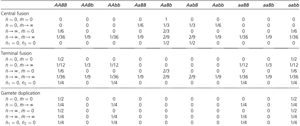
Let us next consider two loci. Offspring proportions when at most one locus is heterozygous can be readily deduced from the single-locus case outlined above. Similarly, when the two loci are on different chromosomes, predicting offspring pro-portions is relatively straightforward because homozygosity will be attained independently at the two loci. When the two loci are on the same chromosome, predicting offspring pro-portions is more complicated. Now there are not two but seven distinct genotypic configurations following prophase of mei-osis I, with transitions between these states induced by cross-overs between the two loci and between the loci and their centromere (Supplemental Material, Figure S1 inFile S2). In Section 1 inFile S1, the expected proportions of these

con-figurations are derived both forfixed numbers of crossovers and assuming again a Poisson distribution of crossovers. Table 1 lists the corresponding proportions of genotypic

A general result from this analysis is that, as expected, the total fraction of offspring that become homozygous at each locus is the same as predicted by the single-locus equations. Thus, in the case of central fusion automixis and denoting byAthe locus that is more closely linked to the centromere than the other locusB, we have

gCF A ¼

1 3

h

12e2ð3n=2Þ

i

and gCF_B ¼1 3

2

4_12e23ðnþmÞ 2

3

5_; (4)

wherenis the expected number of crossovers between the cen-tromere and locusAandm the expected number of crossovers between lociAandB. However, the two rates at which homozy-gosity is attained are not independent. Instead, since the two loci are linked, the fraction of offspring that are homozygous at both loci is greater than what is expected for each locus individually:

gCF AB¼1₃

h

12e2ð3n=2Þ

i 31

3

h

1þ2e2ð3m=2Þ

i .gCF

A gCFB : (5)

With terminal fusion, we obtain

gTF A ¼1₃

h

1þ2e2ð3n=2Þ

i

; gTF

B ¼ 1₃

2

4_1þ2e23ðnþmÞ 2

3

5_{; and}

gTF AB¼1₃

h

1þ2e2ð3n=2Þi31 3

h

1þ2e2ð3m=2Þi.gTF_A gTF_B : (6)

Neutral genetic variation

Let us assume an unstructured,finite population of females repro-ducing through automictic parthenogenesis. We consider a single locus at which new genetic variants that are selectively neutral can arise by mutation at a ratem;and we assume that each mutation produces a new allele (the“infinite alleles-model”). Heterozygosity in individuals may be lost through automixis (with probabilityg), and genetic variation can be lost through drift (determined by population sizeN). We are interested in the equilibrium level of genetic variation that is expected in such a population.

Afirst quantity of interest is the heterozygosityHI;i.e., the

probability that the two alleles in a randomly chosen female are different. Following the standard approach for these type of models (e.g., Hartl and Clark 1997), the change inHIfrom

one generation to the next can be expressed through the change in homozygosity, 12HI;as

12H_I9¼ ð12mÞ212ð12gÞHI : (7)

SolvingHI9¼HIyields the equilibrium heterozygosity

^

HI¼ 12ð12mÞ 2

12ð12mÞ2ð12gÞ 2m

2mþg: (8)

Here, the approximation ignores terms in m2 _{and hence is}

valid for small mutation rates. This approximation illustrates

Table 1 Pos tmeio tic genoty pe con fi gur ations and of fspring genoty pes arisin g from an AaBb mothe r Con fi gur ations after meiosis Proba bility of obtainin g a con fi guration unde r differ ent assum ptio ns abo ut linkage a Resulting of fspring geno type s with di fferent mecha nisms of autom ixis n¼ 0 ; _m¼ 0 n¼ 0 ; m/ N n/ N ; m¼ 0 n/ N ; m/ N

n¼1

0

;

n¼2

0 Cen tral fusion Termina l fusion Gam ete duplica tion AB-AB ab-ab 1 1/6 1/3 1/18 1/2 Only AaBb 1/2 AAB B , 1/2 aabb 1/2 AAB B , 1/2 aabb Ab-Ab aB-aB 0 1/6 0 1/18 1/2 Only AabB 1/2 AAb b , 1/2 aaBB 1/2 AAb b , 1/2 aaBB AB-Ab aB-ab 0 2/3 0 2/9 0 1/4 Aa bb , 1/4 AaBb , 1/4 AabB , 1/4 AaBB 1/2 AAB b , 1/2 aaBb 1/4 AAB B , 1/4 AAb b , 1/4 aaB B , 1/4 aabb AB-a B Ab-a b 0 0 0 2/9 0 1/4 AAB b , 1/4 Aa Bb , 1/4 Aa bB , 1/4 aaBb 1/2 AaBB , 1/2 Aa bb 1/4 AAB B , 1/4 AAb b , 1/4 aaB B , 1/4 aabb AB-a b AB-a b 0 0 2/3 1/9 0 1/4 AA BB , 1/2 Aa Bb , 1/4 aab b Only Aa Bb 1/2 AAB B , 1/2 aabb AB-a b Ab-a B 0 0 0 2/9 0 1/4 AAB b , 1/4 Aa BB , 1/4 Aa bb , 1/4 aaBb 1/2 AaBb , 1/2 Aa bB 1/4 AAB B , 1/4 AAb b , 1/4 aaB B , 1/4 aabb Ab-a B Ab-a B 0 0 0 1/9 0 1/4 AA bb , 1/2 Aa bB , 1/4 aaB B Only Aa bB 1/2 AAb b , 1/2 aaBB

an

1

¼

n¼2

that a balance is reached between the generation of new heterozygotes by mutation (at rate 2m) and their conversion into homozygotes by automixis (at rateg).

Second, we can calculate the probabilityHSthat two alleles

drawn randomly from two different females are different (the“population-level heterozygosity”). The recursion equa-tion forHSis given by

12H9S

¼ ð12mÞ2

1 N

12HI 2

þ

121 N

ð12HSÞ

:

(9)

After substitutingH^Ifrom Equation 8 forHI, the equilibrium

is found to be

^

HS¼12 2gð12mÞ

4_þmð12mÞ2_ð22mÞ

2

h

1þ ðN21Þmð22mÞ

ih

gð12mÞ2þmð22mÞ

i

12 mþg

ð1þ2NmÞð2mþgÞ:

(10)

Again, the approximation is valid for smallmand also assumes thatNis large. Combined, these two quantities allow us to calculate ^FIS; the relative difference between

population-level and individual-population-level heterozygosity at equilibrium:

^

FIS¼HS^ 2HI^ ^

HS ¼

ð2Ng21Þð12mÞ2

ð12mÞ2þ2N

h

gð12mÞ2þmð22mÞ

i

2Ng21

1þ2Nð2mþgÞ:

(11)

Note that as the mutation rate tends to zero,F^ISconverges to ð2Ng21Þ=ð2Ngþ1Þ;and that^FISis negative when 2Ng,1:

Finally, we can calculate the probability H^G that two

ran-domly drawn individuals have a different genotype at the locus under consideration. Unfortunately, this seems to re-quire a more elaborate approach than the simple recursion equations used to calculate H^I andH^S;this approach is

de-tailed in Section 2 inFile S1. The resulting formula is rather cumbersome and not given here, but we can approximate

^

HG assuming that the population size is not too small ðso thatNN21Þbut not too large relative to the mutation rate. This yields the (still unwieldy)

^

HG12N

2_g3_{ð22gÞ þ2mð1þ2NmÞð1þ3NmÞ þgð1þ2NmÞð1þ5NmÞ þNg}2_ð3þ8NmÞ

ð1þ2NmÞ½gþ2mð12gÞ½1þNðgþ3mÞ½1þNgð22gÞ þ4Nm : (12)

Figure 2 shows how the four statistics quantifying different aspects of genetic diversity depend on the rate g at which heterozygosity in individuals is eroded, and compares them to the corresponding statistics in outbreeding sexual popula-tions. Also shown in Figure 2 are diversity estimates from simulations (see Section 3 inFile S1for details), indicating that the analytical predictions are very accurate. It can be seen that both the within-individual and population-level heterozygosities decline with increasingg:Also, the former is greater than the latter for small values ofg; resulting in negative values of^FIS;but this pattern reverses for largerg:In Figure S2 inFile S2, the same relationships are shown but expressed in terms of map distance for the case of central fusion automixis (see Equation 3). These plots illustrate that for the parameters assumed, large between-locus variation in equilibrium genetic diversity is only expected in the close vicinity of the centromeres. Finally, note that the equilibria shown in Figure 2 and Figure S2 inFile S2are reached much more slowly with low than with high values ofg(Figure S3 in

File S2).

Table 2 Total offspring distributions produced by AaBb mother

AABB AABb AAbb AaBB AaBb AabB Aabb aaBB aaBb aabb

Central fusion

n¼0;m ¼0 0 0 0 0 1 0 0 0 0 0

n¼0;m/ N 0 0 0 1/6 1/3 1/3 1/6 0 0 0

n/N;m¼0 1/6 0 0 0 2/3 0 0 0 0 1/6

n/N;m/ N 1/36 1/9 1/36 1/9 2/9 2/9 1/9 1/36 1/9 1/36

n1¼0;n2¼0 0 0 0 0 1/2 1/2 0 0 0 0

Terminal fusion

n¼0;m ¼0 1/2 0 0 0 0 0 0 0 0 1/2

n¼0;m/ N 1/12 1/3 1/12 0 0 0 0 1/12 1/3 1/12

n/N;m¼0 1/6 0 0 0 2/3 0 0 0 0 1/6

n/N;m/ N 1/36 1/9 1/36 1/9 2/9 2/9 1/9 1/36 1/9 1/36

n1¼0;n2¼0 1/4 0 1/4 0 0 0 0 1/4 0 1/4

Gamete duplication

n¼0;m ¼0 1/2 0 0 0 0 0 0 0 0 1/2

n¼0;m/ N 1/4 0 1/4 0 0 0 0 1/4 0 1/4

n/N;m¼0 1/2 0 0 0 0 0 0 0 0 1/2

n/N;m/ N 1/4 0 1/4 0 0 0 0 1/4 0 1/4

n1¼0;n2¼0 1/4 0 1/4 0 0 0 0 1/4 0 1/4

n1¼n2¼0  refers to the case whereAandBare on different chromosomes but each is tightly linked to their centromere. In all other cases the two loci are on the same

To gain further insight into the formulas derived above, it may be helpful to consider a few special cases.

Special case 1:g= 0:This case corresponds to strict clonal

reproduction and has been studied previously (Ballouxet al. 2003). In line with these previous results, all individuals are expected to eventually become heterozygousðH^I¼1Þ;

rep-resenting an extreme case of the Meselson effect (Welch and Meselson 2000; Normarket al.2003). Furthermore, for the equilibrium population-level heterozygosity we get

^

HS1þ4N m

2þ4Nm; (13)

which is always greater than the corresponding genetic di-versity in outbreeding sexual populations½4Nm=ð1þ4NmÞ; see also Figure 2B]. When 4Nmis small,H^S1=2:^FIS

sim-plifies to

^

FIS 2 1

1þ4Nm: (14)

This is always negative because all individuals are heterozy-gous, but alleles sampled from different individuals may still be identical. Finally,

^

HG 4Nm

1þ4Nm; (15)

i.e.,H^Gis identical to the equilibrium heterozygosity in sexual

populations. This is because with strict clonal reproduction, each mutation gives rise to not only a new allele but also to a

new genotype. New diploid genotypes arise twice as often as new alleles in sexual populations, but this is exactly offset by twice the number of gene copies in sexual populations as genotypes in clonal populations.

Special case 2:g= 1 (gamete duplication):This represents

the opposite extreme: barring new mutations, all heterozy-gosity is immediately lost. Thus,H^I¼mð22mÞ 0 and, as a

direct consequence,^FIS1:Moreover,

^

HS 2mN

1þ2mN and HG^ 2mN

1þ2mN: (16)

Not surprisingly,H^SH^G because when all individuals are

homozygous, comparing sampled alleles from different fe-males and comparing genotype samples is equivalent. H^S

andH^G are always lower than the expected heterozygosity

in outbreeding sexual populations. Also note that with

g¼1=2;essentially the same approximations are obtained. This case is genetically equivalent to sexual reproduction with strict selfing, and indeed from the expressions in Ballouxet al.(2003), the above expressions can also be de-rived under this assumption.

Special case 3: N→∞:As the equilibrium heterozygosity is

not affected by population size, Equation 8 remains valid for ^

HI:As expected, bothH^SandH^Gconverge to one asNgoes to

infinity. Finally, we have

^

FIS/ g

2mþg; (17)

Figure 2Equilibrium genetic

diver-sity in neutrally evolving automictic populations, measured as (A) within-individual heterozygosity H^I; (B)

population-level heterozygosity H^S;

(C) relative reduction in heterozygos-ity ^FIS; and (D) diploid

genotype-level diversity H^G: The solid lines

which is equal to the equilibrium individual-level homozy-gosity, 12H^I;and close to one forgm:

Effective population size

The results in the previous section can be put into per-spective by considering the effective population size,Ne, a

commonly used measure for the amount of genetic drift operating within a population. Several definitions for Ne

have been proposed that may or may not be equivalent in different circumstances (Kimura and Crow 1963), but here the most natural choice is the coalescent effective popula-tion size (Nordborg and Krone 2002; Ballouxet al.2003; Sjödin et al. 2005). According to this, Ne is defined as

Ne¼t=2; wheret is the expected time until coalescence

of two randomly chosen alleles in a population. In other words, given thatt¼2Nin the standard coalescent with Ndiploid individuals,Neis defined through a rescaling of

time in a complex population model so that this population behaves like a Fisher–Wright population with respect to coalescent times.

For asexual populations, it is useful to further distinguish between a genotypic and an allelic effective population size (Ballouxet al. 2003). The genotypicNeis based on

coales-cence of diploid genotypes, and in asexual populations is given simply by Ne¼N=2 for both clonal (Balloux et al.

2003) and automictic populations. This is because instead of sampling 2Nalleles every generation in sexual popula-tions,Ngenotypes are sampled in clonal populations so that drift is stronger and coalescence times are shorter. This pro-vides an alternative explanation for the expressions for H^G

obtained above. With clonal reproduction, the mutation rate for diploid genotypes is twice the mutation rate for alleles in sexual populations, but the effective population size is only half that of a sexual population, so thatH^Gis the same as the

equilibrium heterozygosity in outbreeding sexual popula-tions. With gamete duplication, the genotypic mutation rate is effectively the same as the allelic mutation rate (because half of the mutations are immediately lost), so thatH^Gcan be

obtained from the classic equilibrium heterozygosity in sex-ual populations by replacing Nwith Ne¼N=2:In general,

automixis itself is not part of the coalescence process from a genotypic point of view but rather contributes, along with mutation, to switches between different genotypes.

To obtain the allelic effective population size we can distinguish between two situations. First, the two alleles sampled may both reside within the same female. This occurs with probability 1=N;and given that going backward in time the two alleles coalesce with probabilitygin each generation, the expected coalescence time in this case is 1=g:Second, the two alleles may be sampled from different females (with probability 121=NÞ: In this case, coalescence of the two genotypic lineages has to occurfirst (this will take on average Ngenerations), and when this has happened the two alleles may either have also coalesced simultaneously (with proba-bility 1/2), or it may again take an expected number of 1=g generations for coalescence to occur. In total we get

t¼1 N

1

gþ

121 N

Nþ1 2

1

g

; (18)

which translates into an allelic effective population size of

Ne¼t

2 ðN=2Þ þ 1

4g: (19)

Thus, in contrast to the genotypicNe;the allelicNedepends on g so that different loci within the genome may experience different levels of genetic drift in relation to their distance from the centromere. With gamete duplicationðg¼1Þthe allelic effective size is around N=2; i.e., the same as the genotypic effective size and half the effective size of a stan-dard Fisher–Wright population. As g decreases, the allelic effective population size increases, reaching that of the Fisher–Wright population for g1=ð2NÞ (which may be attained for some loci under central fusion automixis) and then increasing further to infinity as g approaches zero (clonal reproduction; see also Ballouxet al.2003). This

re-flects the expectation that for clonally or near clonally inherited loci, the two gene copies within a genotypic line will never, or only after a very long time, coalesce. As shown in the previous section (and Figure 2, A and B), this results in within-individual heterozygosity levels near one and also high population-level heterozygosity.

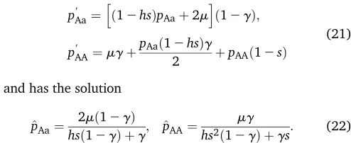
Mutation–selection balance

To investigate the balance between the creation of deleterious alleles through mutation and their purging by natural selec-tion in automictic populaselec-tions, let us assume an infinitely large population and a single locus with two allelesa(wild type) and A (deleterious mutation). Wild-type aa individuals have a fitness of waa¼1 relative to heterozygotes with

wAa¼12hs and mutant homozygotes with wAA¼12s:

To keep the model tractable, I assume that the mutation rate

mis small so that at most one mutation event occurs during reproduction, and that there is no back mutation from mu-tant to wild-type allele. Automixis operates as in the previous section, with heterozygotes producing a fractiong=2 of either homozygote. Assuming a life-history order of selection, mu-tation, and automixis, the recursion equations for the fre-quencies of the two mutant genotypes can be expressed as

p9Aa¼

h

ð12hsÞð12mÞpAaþ2mð12pAa2pAAÞ

i

ð12gÞ

12hspAa2spAA ;

p9AA¼

mgð12pAa2pAAÞ þ ð12hsÞ

_g

2þm

12g₂pAaþpAAð12sÞ

12hspAa2spAA :

(20)

Solvingðp9Aa;pAA9 Þ ¼ ðpAa;pAAÞ yields the frequencies of the

mutant genotypes under the mutation–selection equilibrium. Unfortunately, the resulting formulas are rather uninforma-tive and not given here. However, we can make progress by linearizing Equations 20 under the assumption that m;pAa;

will be met ifmsand ifgis not too small. This approxi-mation reads

p9_Aa¼hð12hsÞpAaþ2mið12gÞ;

p9_AA¼mgþpAað12hsÞg

2 þpAAð12sÞ

(21)

and has the solution

^ pAa¼

2mð12gÞ

hsð12gÞ þg; ^pAA¼

mg

hs2_{ð12gÞ þgs}: (22)

It may be informative to consider a few special cases where tractable results can also be obtained directly from the solu-tion to system (20).

Special case 1: Clonal reproduction (g= 0):In this case,

the equilibrium that will be attained depends on the magni-tude of the mutation rate. First, when the mutation rate is small,m#hs=ð1þhsÞ;we get

^

p_Aa¼ 2mðs22mÞ

sfhsþm½12hð2þsÞg 2m

hs;

^ pAA¼

2m2ð12hsÞ

sfhsþm½12hð2þsÞg0:

(23)

At this equilibrium, the population will consist mostly of mutation-freeaaindividuals, with some heterozygotes and very few AA homozygotes. Note that^pAais approximately the

same as the equilibrium frequency of heterozygotes in an outbreeding sexual population.

Second, when hs=ð1þhsÞ,m#s=2; the equilibrium is given by

^

pAa¼12

mð12hsÞ

ð12hÞs; ^pAA¼

mð12hsÞ

ð12hÞs: (24)

No mutation-free aa individuals persist in the population in this case (sincep^Aaþ^pAA¼1Þ:Intuitively, this situation

arises when selection against heterozygotes is so weak rela-tive to the mutation rate that eventually allaaindividuals are converted into heterozygotes and a mutation–selection bal-ance is attained betweenAaandAAindividuals. This balance is then analogous to the standard mutation–selection balance in haploid populations. Indeed, after renormalizing allfitness values with the fitness of heterozygotes and defining an adjusted selection coefficient against AA homozygotes, ~s¼12ð12sÞ=ð12hsÞ;the equilibrium frequency of homo-zygous mutants can be expressed as^pAA¼m=~s:Finally, when m.s=2; the mutation pressure outweighs selection com-pletely and the mutant homozygotes will become fixed in the populationð^pAA¼1Þ:

Special case 2: Gamete duplication (g= 1):At the opposite

extreme, when all heterozygotes are immediately converted into homozygotes, the equilibrium frequencies are given by

^

pAa¼0; ^pAA¼

m

s: (25)

It is clear that in this case, selection against heterozygotes and thus the dominance coefficienthis irrelevant. Mutation-free aa homozygotes produce heterozygote mutant offspring at a rate 2mper generation, but these heterozygotes are immedi-ately converted into aa andAAoffspring, each with probabil-ity 1/2. Thus, the effective rate at which AA offspring are produced ism and the attained mutation–selection balance is identical to the one attained in haploid populations.

Special case 3: Recessive deleterious mutations (h = 0):

With arbitrary values of gbut strictly recessive deleterious mutations, the equilibrium is given by

^ pAa¼

2mðs2mÞð12gÞ

sgþmð223gÞ ; ^pAA¼

m

s: (26)

Thus, the equilibrium frequency^pAAof mutant homozygotes

is identical to the one expected in sexual populations with recessive deleterious mutations(corresponding to an equilib-rium allele frequency of ^pA¼

ffiffiffiffiffiffiffiffi m=s

p

Þ:The equilibrium fre-quency of heterozygotes is a decreasing function ofgand can be either higher or lower than the corresponding equilibrium frequency of heterozygotes in sexual populations.

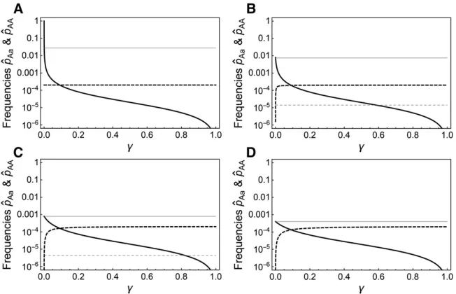
Figure 3 shows equilibrium frequencies of theAaandAA genotypes under mutation–selection balance for recessive, partially recessive, semidominant, and dominant mutations, and compares these frequencies to the corresponding fre-quencies in sexual populations. For g.0;the frequency of heterozygotes is generally lower than in sexual populations, whereas the frequency ofAAhomozygotes is higher than in sexual populations. Related to this, the equilibrium frequen-cies in automictic populations are generally much less sensi-tive to the dominance coefficienththan in sexual populations becauseg.0 implies that selection against heterozygotes is much less important than in sexual populations. Also note that populations reproducing by strict selfing (corresponding tog¼1=2Þare characterized by very similar frequencies of AAhomozygotes as automictic populations with high values ofg; while the frequencies of heterozygotes are very low in both cases.

The equilibrium frequencies can also be used to calculate the mutational load Lmut;i.e., the relative reduction in the

meanfitness of the population caused by recurrent mutation. This quantity can be expressed as

Lmut¼12w¼hsp^Aaþs^pAAm

2hsð12gÞ þg hsð12gÞ þg:

From this and Equations 25 and 26 it can be deduced that both with gamete duplication ðg¼1Þ and recessive mutations

ðh¼0Þ;the genetic load in the population is given by the mutation ratem; the same as for recessive mutations in sex-ual diploid populations and also the same as in haploid pop-ulations. In general, Lmut will be greater thanmbut always

load in clonal diploids in which the maintenance of hetero-zygosity caused the asexual populations to accumulate a higher load than the sexual populations (Chasnov 2000; Haag and Roze 2007). It is important to note, however, that the simple results derived here do not account forfinite pop-ulation size and interference between multiple loci, which may have a strong impact on the mutation–selection balance and the mutational load (Glémin 2003; Haag and Roze 2007; Roze 2015).

Overdominance

When there is overdominance (i.e., a heterozygote fitness advantage over the homozygote genotypes), it is useful to parameterize the fitness values as waa¼12saa; wAa¼1;

andwAA¼12sAA;with 0,saa; sAA#1:The recursion

equa-tion for the genotype frequenciespAa andpAA can then be

expressed as

p9Aa¼

ð12gÞpAa

12ð12pAA2pAaÞsaa2pAAsAA;

p9_AA¼ ð12sAAÞpAAþpAag=2 12ð12pAA2pAaÞsaa2pAAsAA:

(27)

Solvingðp9Aa;pAA9 Þ ¼ ðpAa;pAAÞyields the following

polymor-phic equilibrium:

^ pAa¼

2ðsaa2gÞðsAA2gÞ

2saasAA2gðsaaþsAAÞ; ^pAA¼

gðsaa2gÞ 2saasAA2gðsaaþsAAÞ:

(28)

This equilibrium takes positive values forg,saaandg,sAA;

and stability analysis indicates that this is also the condition for the equilibrium to be stable. [The eigenvalues of the associated Jacobian matrix areð12saaÞ=ð12gÞandð12sAAÞ=ð12gÞ:

Thus, overdominant selection can maintain heterozygotes in the face of erosion by automixis if the selection coefficient against both homozygotes is greater than the rate at which heterozygosity is lost. This result has previously been

conjectured by Goudieet al.(2012) on the basis of numerical results of a similar model, and more complex expressions for equilibrium (28) have been derived by Asher (1970).

Depending ong;the equilibrium frequency of heterozygotes can take any value between 0ðwheng$minfsaa;sAAgÞand 1 (when g¼0;i.e., with clonal reproduction). This is shown in Figure 4 and contrasted with the equilibrium frequency in outbreeding sexual populations, given by 2saasAA=ðsaaþsAAÞ2:

We can also calculate how much the meanfitness in the population at equilibrium is reduced by automixis compared to clonal reproduction. Provided thatg,saa;sAA;this“

auto-mixis load”is given by

Lautomixis¼12^pAA2^pAa

saa2^pAAsAA¼g: (29)

This simple formula parallels the classic result that the mu-tational load in haploid populations is given by the mutation rate and thus shows that automixis acts like mutation in producing two genotypes (AAandaa), of inferiorfitness from the fittest genotype (Aa), that are then purged by natural selection. The genetic load can be either smaller or greater than the corresponding segregation load in a sexual popu-lation. More precisely, when g,Lseg¼saasAA=ðsaaþsAAÞ

(Crow and Kimura 1970), there will be more heterozygotes in the automictic population and their genetic load will be lower than in the sexual population, and vice versa. When

g.minfsaa;sAAg;the heterozygotes are lost from the

popu-lation and either the aa (ifsaa,sAA) or theAAgenotype (if

saa . sAA) will become fixed. In this case, we obtain the

largest possible load,Lautomixis¼ minfsaa;sAAg.

Associative overdominance

In addition to overdominance, heterozygosity could also be maintained through off-phase recessive deleterious mutations at tightly linked loci (Frydenberg 1963; Ohta 1971), and this has been proposed to explain heterozygosity in the Cape honeybee (Goudie et al.2014). Consider a recently arisen

Figure 3 Equilibrium genotype frequencies under

lineage reproducing through central fusion automixis in which, by chance, the founding female carries a strongly del-eterious recessive mutation Aon one chromosome and an-other strongly deleterious recessive mutation Bat a tightly linked locus on the homologous chromosome. Thus, the genetic constitution of this female is AabB. Then, the vast majority of offspring that have become homozygous for the high-fitness alleleaare also homozygous for the deleterious alleleB and vice versa, so that linkage produces strong in-direct selection against bothaaandbbhomozygotes.

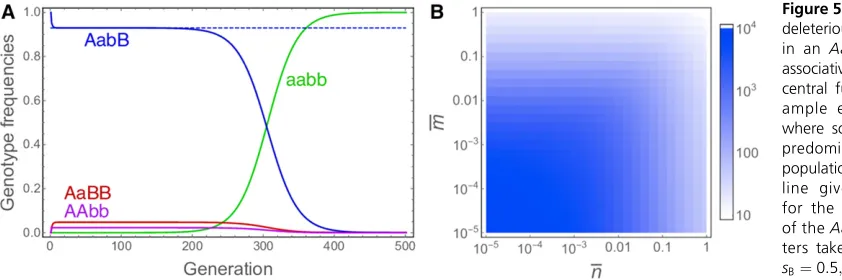
To investigate this mechanism, numerical explorations of a two-locus model of an infinitely large population undergoing selection and reproduction through automixis were per-formed. This model builds upon the expressions for loss of heterozygosity in the presence of recombination between a centromere and two loci derived above (for details see Section 4 inFile S1). Heterozygosity at either locus entails a reduc-tion offitness of 12hisiði2 fA;BgÞ;whereas homozygosity for the deleterious alleles reduces fitness by 12si in each locus. Fitness effects at the two loci are multiplicative (i.e., no epistasis). An example run is shown in Figure 5A. As can be seen, theAabBgenotype is maintained at a high frequency for a considerable number of generations (in automixis– selection balance with the two homozygous genotypesAAbb andaaBB) before it is eroded by recombination between the two loci and theaabbgenotype spreads tofixation. We can also treat the two linked loci as a single locus and use the equilibrium frequency of heterozygotes derived above for single-locus overdominance to estimate the quasi-stable fre-quency of theAabBgenotype before it is dissolved. Specifi -cally, this frequency can be approximated by Equation 28 following substitution ofsAA forsB;saa forsA;andg for

the expression in Equation 3, yielding

pAabB

2

h

1þ3sA2expð23n=2Þ ih

1þ3sB2expð23n=2Þ i

18sAsBþ3ðsAþsBÞ h

12expð23n=2Þ

i :

(30)

For simplicity, this approximation assumes complete recessiv-ityðhA¼hB¼0Þ;but partial recessivity could also readily be incorporated. As shown in Figure 5A, this approximation is very close to the quasi-stable frequency of theAabBgenotype obtained numerically.

Next, we can ask for how long the AabB genotype is expected to persist in the population. To address this ques-tion, screens of the parameter space with respect to the two mean crossover numbers were performed. The recursion equations were initiated with onlyAabBindividuals present in the population and iterated until their frequency dropped below 0.01. The number of generations this took for different mean numbers of crossoversnbetween locusAand the cen-tromere and different numbers of crossoversm between loci

AandBare shown in Figure 5B. It can be seen that, provided the two loci are both tightly linked to the centromere, central fusion automixis can indeed maintain the polymorphism for many generations. The same principle also applies to termi-nal fusion automixis and sexual reproduction, but here the deleterious recessive mutations are only maintained for very short time periods (results not shown).

Spread of beneficial mutations

To better understand adaptive evolution in automictic pop-ulations, consider first a deterministic single-locus model without mutation and with relativefitness 1þhsand 1þs for heterozygotes andAAhomozygotes, respectively. Analo-gously to Equations 20 for deleterious mutations (but assum-ing a mutation rate of zero), the recursion equations for this model can then be written as

p9_Aa¼ð1þhsÞð12gÞpAa 1þpAahsþpAAs ;p

9

AA¼

ð1þhsÞgpAa=2þ ð1þsÞpAA 1þpAahsþpAAs :

(31)

Assuming that both theAaand theAAgenotype are rare in the population and thatsis small, these recursion equations can be approximated by

p9_Aa ð1þhsÞð12gÞpAa;p9_AA¼1

2ð1þhsÞgpAaþ ð1þsÞpAA: (32)

This linear system of recursion equations can be solved, and if we further assume that initially there are only one or few heterozygote mutants but noAAhomozygotes½pAAð0Þ ¼0; this solution becomes

pAaðtÞ ¼pAað0Þktand

pAAðtÞ ¼pAað0Þð1þhsÞg

ð1þsÞt2kt

2ð1þs2kÞ ;

(33)

with k:¼ ð1þhsÞð12gÞ: These expressions demon-strate that whengis large relative to the selection

bene-fit of heterozygotes—more precisely when k,1; or

g. hs

1þhshs—the heterozygotes will not be maintained and the beneficial mutation will instead spread as a

Figure 4 Equilibrium heterozygote frequencies under overdominant

selection and for given rates gat which heterozygotes are converted into homozygotes. The bold lines show these frequencies under auto-mictic reproduction and forsAA¼saa¼0:9 (solid line),sAA¼saa¼0:5

(dashed line), and sAA¼1; saa¼0:2 (dotted line). For comparison,

homozygous genotype through the population. Thus, in this case we have for sufficiently larget:

pAaðtÞ 0 and pAAðtÞ pAað0Þ ð1þhsÞg 2ð1þs2kÞð1þsÞ

t_:

(34)

Here,handgdetermine how efficiently the initial heterozy-gotes are maintained and converted to homozyheterozy-gotes, but onlysdetermines the actual rate at which the beneficial mu-tation spreads. By comparison, a beneficial mutation in an outbreeding sexual population will initially be found in het-erozygotes only, with

pAaðtÞ pAað0Þð1þhsÞt: (35)

Thus, the rate at which the mutation spreads in sexual pop-ulations is determined by thefitness advantage in heterozy-gotes only, which means the mutation will always spread at a lower rate than in automictic populations. Nevertheless, the heterozygotes in sexual populations have a“head start” rel-ative to the homozygotes in automictic populations (see frac-tion in Equafrac-tion 34), which results from the fact that only half of the original heterozygotes are converted into homozy-gotes. This means that with high dominance levelsh, it might still take some time until a beneficial allele reaches a higher frequency in an automictic compared to a sexual population.

When 0,g, hs

1þhshs; both heterozygotes andAA ho-mozygotes will spread simultaneously in the population and, for very smallg;it may take a long time until the homo-zygotes reach a higher frequency than the heterohomo-zygotes. In the extreme case of g¼0 (clonal reproduction), heterozy-gote frequency increases by a factor ofð1þhsÞin each gen-eration (i.e., at the same rate as in outbreeding sexuals), and no homozygotes are produced.

The above considerations apply only to the early phase of the deterministic spread of a beneficial mutation destined to spread in a population. In a more realistic setting involving random genetic drift, we can also ask what thefixation prob-ability of beneficial mutations is in automictic populations.

Assuming that offspring numbers of rare mutant females are distributed independently, we can treat the spread of benefi -cial mutations as a multi-type branching process (e.g., Allen 2003, Chap. 4). (Note that this approach is valid for large populations; for small populations different approaches that take the effective population size into account will provide better approximations.) Building on Equation 32, the mean numberMijof offspring of typej(1 =Aa, 2 =AA) produced by a mother of typeiis given by the matrix

M¼

ð1þhsÞð12gÞ ð1þhsÞg=2

0 1þs

: (36)

Assuming that offspring numbers follow Poisson distributions with these means, we arrive at the following probability-generating functions for the branching process:

f1ðq1;q2Þ ¼eð1þhsÞð12gÞðq121Þ_e

ð1þhsÞgðq₂21Þ

2 ;

f2ðq1;q2Þ ¼eð1þsÞðq221Þ:

(37)

Simultaneously solving

f1ð12U1;12U2Þ ¼12U1and

f2ð12U1;12U2Þ ¼12U2 (38)

then yields thefixation probabilitiesU1andU2when there is

initially a single Aa or AA mutant individual, respectively. Equations 38 can only be solved numerically. However, as-suming weak selection, series expansion off2and retaining

only quadratic and lower terms gives the approximation U22s;mirroring a well-known result in haploid

popula-tions. Substituting 2sforU2in the expression forf2;

expand-ing, and again retaining only quadratic or lower terms then gives the biologically more interesting

U1

wð12gÞ2eswgþ

ffiffiffiffiffiffiffiffiffiffiffiffiffiffiffiffiffiffiffiffiffiffiffiffiffiffiffiffiffiffiffiffiffiffiffiffiffiffiffiffiffiffiffiffiffiffiffiffiffiffiffiffiffiffiffiffiffiffiffiffiffiffiffiffiffiffiffiffiffiffiffiffiffiffiffiffiffiffiffiffiffiffiffiffiffiffiffiffiffiffiffiffiffiffiffi

e2swg_2w2_ð12gÞ2_ð

122eswgÞ22wð12gÞeswg

q

w2_ð12gÞ2 ;

(39)

with placeholder w:¼1þhs: When g is not too small, this expression can be further approximated by Taylor

Figure 5Maintenance of strongly

deleterious mutations (A and B) in an AabB genotype through associative overdominance with central fusion automixis. (A) Ex-ample evolutionary dynamics where solid lines show the four predominant genotypes in the population and the dashed blue line gives the approximation for the quasi-stable frequency of theAabBgenotype. Parame-ters take the values sA¼0:999;

sB¼0:5; hA¼hB¼0; n¼0:1;

andm¼1027_{:(B) Time until}

expansion ins(discarding terms above second order) to yield

U1s

12s122h 2g

: (40)

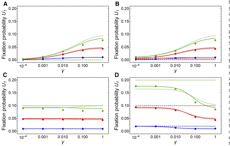
Figure 6 illustrates both Equation 39 and numerical solutions of Equations 38 for thefixation probability of a new beneficial mutation. Figure 6 also shows that unless selection is strong, there is a good correspondence between these results based on the branching process approximation and simulation re-sults. It can be seen that for recessive and partially recessive mutations, thefixation probability increases with increasing

gand is greater than thefixation probability in outbreeding sexual populations (Figure 6, A and B). Beneficial mutations with additive effects are relatively insensitive to g (Figure 6C), and for dominant mutations thefixation probability de-creases with increasing g:The approximation in Equation 40 also illustrates the dependency ofU1 ong for different

dominance levels. In all cases, thefixation probability con-verges toU1sasgapproaches 1. This is rather intuitive as

withg¼1 (i.e., gamete duplication), anAafemale produces an AA offspring individual with a probability of approxi-mately 1/2 in thefirst generation, upon which theAA geno-type thenfixes in the population with probability2s:When

g¼1=2;corresponding to strict selfing, thefixation proba-bility is already close to U1s;as has been derived

previ-ously (Charlesworth 1992).

The above considerations demonstrate that unless benefi -cial mutations are completely dominant, their deterministic spread is expected to be faster in automictic than in either clonal or sexual populations. For recessive or partially re-cessive beneficial mutations, this also translates into a higher probability offixation. To what extent do these results hold when more than one locus is considered? It is well known that asexually reproducing populations may fix beneficial mu-tations more slowly because of clonal interference, i.e., competition between simultaneously spreading beneficial mutations that, in the absence of recombination, cannot be brought together into the same genome (Fisher 1930; Muller 1932). Despite the term “clonal interference,” this mecha-nism should also operate in automictic populations, and we can ask whether and under what conditions the decelerating effect of clonal interference on the speed of adaptive evolu-tion can offset the beneficial effects of turning heterozygotes with one beneficial mutation into homozygotes with two ben-eficial mutations.

To address this question, numerical investigations of a two-locus model involving recombination, automixis, selection, and drift were performed. (Note that clonal interference only operates infinite populations subject to random genetic drift and/or random mutations.) Full details of this model can be found in Section 5 inFile S1. The results of a screen of the two crossover numbersn(between locusAand the centromere) and crossoversm (between lociAandB) are shown in Figure S5 inFile S2. It appears that unlessnis very small, recessive

beneficial mutations spread considerably faster in automictic than in sexual populations, despite clonal interference in the former. With additivefitness effects, the difference between automictic and sexual populations is less pronounced and the beneficial effects of recombination become apparent whenn is very small. Perhaps surprisingly, the mean number m of crossovers between the two loci under selection, which de-termines the recombination rate in the sexual population, plays only a minor role and needs to take low values for re-cessive beneficial mutations to spread slightly faster in sexual than automictic populations (bottom-left corner in Figure 6A). This is because although increasing values ofm lead to faster spread of the beneficial mutations in sexual popula-tions, this effect is only weak compared to the accelerating effect of increasingm in automictic populations.

The results obtained in this section regarding the spread of beneficial mutations are only a step toward understanding adaptive evolution in automictic populations. Further prog-ress should be made by deriving expprog-ressions forfixation and extinction times (see, e.g., Mandegar and Otto 2007 and Glémin 2012 for the related cases of clonal reproduction with mitotic recombination and selfing, respectively), by consid-ering many loci (see Pamiloet al.1987 for some results on automictic populations for mutations with additive fitness effects), and by developing models for the recurrent spread of beneficial mutations with variablefitness effects (see,e.g., Kim and Orr 2005 for a comparison between sexual and clonal populations).

Selection on crossover rates

Wefinally turn to the question of whether natural selection is expected to reduce crossover rates in automictic populations. Let usfirst consider a population reproducing by central fusion automixis in which heterozygosity at a given locus is main-tained through overdominant selection. Combining the re-sults from Equations 3 and 29, the meanfitness of a resident population with a mean crossover numbernis given by

w¼12g¼1 3

"

2þexp

23n

2

#

: (41)

Since reproduction is asexual and assuming a dominant cross-over modifier allele, the selection coefficient sfor a mutant genotype with a different crossover rate can be obtained sim-ply by comparing the mean fitness of the resident and the mutant lineage. [This is in contrast to recombination rate evo-lution in sexual populations, where a much more sophisticated approach is required (Barton 1995).] If the factor by which crossover numbers are altered is denoted bya(i.e., the mutant mean number of crossovers isanÞ;this yields

s¼exp

23an 2

2exp23n₂ 2þexp23n₂

1

2ð12aÞn; (42)

selectively favored ðs.0Þ: In the extreme case of a¼0 (complete crossover suppression),

s¼12exp

23n

2

2þexp23n

2

; (43)

which ranges from around n=2;when the initial crossover rate is already very small, to 1=2;whennis very large.

With terminal fusion automixis, we obtain

s¼e2 3n

22e2 3an

2

12e232n

a21: (44)

Again, the approximation is valid for smalln(but note that conditions where overdominance stably maintains heterozy-gosity are rather limited in this case; see Equation 26). In-creases in crossover rates are selected for with terminal fusion, but even when there are many crossovers between the focal locus and its centromere, a substantial genetic load

ðL¼1=3Þwill persist.

We can also ask how selection should operate on crossover rates in automictic populations evolving under mutation– selection balance. Without answering this question in any quantitative detail, we can note that since the equilibrium genetic load decreases with increasing g(Figure S4 in File S2), there should be selection for increased crossover rates in populations with central fusion automixis and selection for decreased recombination rates in populations with terminal fusion automixis. However, given that genetic load is always in the range betweenmand 2m;selection for increased cross-overs will be only very weak on a per-locus basis ðs,mÞ: Stronger selection is expected when there are preexisting

deleterious mutations at high frequencies (e.g., following the emergence of a new, genetically uniform automictic line-age). For example, with partially recessive mutations and central fusion automixis, there may initially be strong selec-tion against crossovers (avoiding the unmasking of the mu-tation in heterozygotes), followed by selection for increased crossover rates (enabling more efficient purging of the mu-tation). Preliminary numerical investigations competing two lineages with different crossover rates confirm these predic-tions on selection on crossover rates (e.g., Figure S6 inFile S2). However, it will be important to study this problem more thoroughly in a multi-locus model and withfinite populations so that, for example, the impact of stochastically arising as-sociative overdominance can also be ascertained.

Data availability

The authors state that all data necessary for confirming the conclusions presented in the article are represented fully within the article. Most results were obtained using Mathe-matica v.10 (Wolfram Research Inc.); the MatheMathe-matica note-book is available at https://github.com/JanEngelstaedter/ AutomixisEvolution.

Discussion

Automixis as a viable system of reproduction

Automixis is a peculiar mode of reproduction. Not only are, as with other modes of asexual reproduction, the benefits of recombination forfeited, but the fusion of meiotic products to restore diploidy also means that heterozygosity can be lost at a high rate. This raises intriguing questions as to why automixis

Figure 6 Fixation probabilities of

has evolved numerous times and how stably automictically reproducing populations can persist. Previous work has shown that the loss of complementation faced by a newly evolved automictically reproducing female can cause severe reduc-tions infitness that may exceed the twofold cost of sex, and are likely to severely constrain the rate at which sex is abandoned (Archetti 2004, 2010; Engelstädter 2008). However, the re-sults obtained here indicate that once an automictic popula-tion is established, it may persist and in some respects even be superior to clonal or sexual populations. In particular, neutral genetic diversity will be lower in automictic than in clonal populations but may still be greater than in sexual popula-tions, the mutational load will generally be lower in automic-tic than in both sexual and clonal populations (unless mutations are completely recessive), and the genetic load caused by overdominant selection can be lower in automictic than in sexual populations.

Empirical examples confirming that automicts can be highly successful at least on short to intermediate timescales include the Cape honeybee clone (which has been spreading for.25 years) (Goudie and Oldroyd 2014), the invasive ant Cerapachys biroi(which has been reproducing asexually for at least 200 generations) (Wettereret al.2012; Oxleyet al. 2014), and Muscidifurax uniraptorwasps which have been infected by parthenogenesis-inducing Wolbachia for long enough that male functions have degenerated (Gottlieb and Zchori-Fein 2001). Of course, automictic populations still suffer from the lack of recombination and hence long-term consequences such as the accumulation of deleterious mutations through Muller’s ratchet or reduced rates of adap-tation because of clonal interference. It therefore does not come as a surprise that, like other asexuals, automictic spe-cies tend to be phylogenetically isolated (Schwander and Crespi 2009). One exception to this rule are the oribatid mites, in which10% out of.10,000 species reproduce by automixis and radiations of automictic species have occurred (Domeset al.2007; Heethoffet al.2009). To better under-stand the long-term dynamics of adaptation and mutation accumulation in automictic populations, it would be useful to develop more sophisticated models than presented here that incorporate multiple loci and random genetic drift.

Relationship to other genetic systems

There is a bewildering diversity of genetic systems that have similarities to automixis. To discuss the relationship of the results obtained here with prior work it may be useful to group these genetic systems into two classes. Thefirst are systems that are mechanistically distinct from automixis but are ge-netically equivalent. This includes systems in animals and plants where there is no fusion of meiotic products but some other meiotic modification that has the same consequences, and also systems of intratetrad mating. The results obtained here are thus directly applicable, and previous theoretical work on such systems can directly be compared to the work presented here. For example, parthenogenesis in Daphnia pulex has been reported to proceed through a modified

meiosis in which thefirst anaphase is aborted halfway, ho-mologous chromosomes are rejoined, and the second meiotic division proceeds normally (Hiruta et al. 2010). Similarly, some forms of apomixis in plants (meiotic diplospory) are also achieved by suppression of the first meiotic division (Gustaffson 1931; van Dijk 2009). These modifications of meiosis are genetically equivalent to central fusion automixis and can, through complete suppression of recombination, also lead to clonal reproduction. Intratetrad mating is com-monly found in many fungi, algae, and other organisms and is achieved through a variety of mechanisms (Kerrigan et al. 1993; Hood and Antonovics 2004). Provided the mating-type locus is completely linked to the centromere, intratetrad mating is genetically equivalent to central fusion automixis (Antonovics and Abrams 2004). If the mating-type locus is not closely linked to the centromere, the outcome would still be equivalent to automixis but with a mixture of terminal and central fusion, depending on whether or not there has been a recombination event between the mating-type locus and the centromere. Finally, systems of clonal reproduction with mi-totic recombination should also be equivalent to central fusion automixis; here, heterozygosity is also lost with probability 1/2 during one of the mitoses in the germline when there was a recombination event between a locus and its associated centromere (Mandegar and Otto 2007).

The second class of systems comprises those that are very similar to automixis but equivalent only when a single locus is considered. This means that many of the results reported here (e.g., on neutral variation, mutation–selection balance, and overdominance) can still be applied. For example, clonal pop-ulations in which there is occasional, symmetrical gene con-version can be considered genetically equivalent to the single-locus models considered here, with the rate of loss of heterozygositygreplaced by the gene conversion rate. Gene conversion has been reported in several parthenogenetic an-imals (Crease and Lynch 1991; Schon and Martens 2003; Flot et al. 2013), and recently a number of results concerning coalescent times and patterns have been derived for such systems (Hartfieldet al.2016).

2015). The only exceptions to this rule are automictic pop-ulations reproducing by gamete duplication (whereg¼1 for all loci), and when gametic products fuse randomly (resulting ing¼1=3 for all loci).

Populations with mixed automictic and sexual reproduction

The models presented here assume populations that repro-duce exclusively through automixis. Although several species with exclusively automictic reproduction have been reported, many other species exhibit different forms of mixed sexual and automictic reproduction. The simplest case is one where a lineage of automicts competes with sexual conspecifics but where there is no geneflow between these two populations. Such a situation is found in the Cape honeybee,A. mellifera capensis, in which a subpopulation (the clone) reproduces through central fusion automixis and parasitizes colonies of a sexual subspecies, A. mellifera scutellata (Goudie and Oldroyd 2014). In principle, the results presented here could be used to predict the outcome of such competitions by com-paring population meanfitness of sexual and automictic pop-ulations. However, the case of the Cape honeybee is fraught with a number of additional complexities, including both honeybee characteristics such as eusociality and the comple-mentary sex determination system, as well as the parasitic nature and epidemiological dynamics of the clone. This will make it necessary to develop specifically tailored models that incorporate both the evolutionary genetics consequences of automixis explored in the present article and the ecological and genetic idiosyncrasies of the clone (Martinet al.2002; Moritz 2002).

More complicated is the case of gene flow between the sexual and automictic subpopulations. This can occur, for example, when otherwise automictic females occasionally produce males. Provided these males are viable and fertile, they may mate and produce offspring with the sexual females. This will not only introduce genetic material from the asexual into the sexual populations, but it may also lead to the emergence of new automictic lineages because the males may transmit the genes coding for automictic reproduction to their female offspring. Such cases of “contagious parthe-nogenesis” (Simon et al. 2003) associated with automixis have been reported in the parasitoid waspLysiphlebus faba-rum(Sandrock and Vorburger 2011; Sandrocket al.2011) and Artemiabrine shrimps (Maccariet al.2014). Some as-pects of the evolutionary dynamics of such systems have been studied (Engelstädter et al. 2011), but population genetic processes such as the ones studied here remain to be investigated.

Finally, there are many species in which there are no clear sexual and asexual subpopulations but where females can reproduce both sexually and through automixis. This includes, for example, the majority ofDrosophilaspecies where parthe-nogenesis has been reported (Markow 2013), and also a num-ber of vertebrates with facultative parthenogenesis (Lampert 2008). It is expected that sexual populations capable of

occasional automictic reproduction should not differ much from sexual populations in terms of population genetic processes. One exception is that rare automixis may facilitate the colo-nization of previously uninhabited areas. Distinguishing the genomic signature of the resulting automictically arisen pop-ulation bottlenecks from those of“conventional”bottlenecks will be challenging but may be feasible with data on genome-wide levels of heterozygosity (see also Svendsenet al.2015). On the other hand, rare sex in predominantly automictic populations is expected to have a great impact as the mixing of lineages may efficiently counteract clonal interference and Muller’s ratchet (Hojsgaard and Horandl 2015).

Conclusions

In this study, a number of theoretical results regarding basic population genetic processes in automictic populations were derived for both neutral and selective processes. A general conclusion that emerges is that, in analogy to strong levels of inbreeding, automictic reproduction is difficult to evolve but once established may be viable on intermediate timescales and even has advantages compared to clonal and sexual reproduction. Future theoretical work is still necessary to elucidate long-term evolutionary patterns of automictic spe-cies, such as the rate of mutational meltdown under Muller’s ratchet or the dynamics of adaptation.

Acknowledgments

I thank Christoph R. Haag, Nicholas M. A. Smith, and two anonymous reviewers for their insightful comments on the manuscript. One of the anonymous reviewers provided particularly helpful advice on obtaining compact approxi-mations for some of the analytical results. I thank Isabel Gordo and the Instituto Gulbenkian de Ciência (Portugal) for hosting me during thefinal stages of preparing this man-uscript. The author declares no conflict of interest.

Literature Cited

Allen, L. J. S., 2003 An Introduction to Stochastic Processes with Applications to Biology. Pearson/Prentice Hall, Upper Saddle River, NJ.

Allsopp, M., 1992 The Capensis calamity. South Afr. Bee J. 64: 52_–55. Antonovics, J., and J. Y. Abrams, 2004 Intratetrad mating and the

evolution of linkage relationships. Evolution 58: 702–709. Archetti, M., 2004 Recombination and loss of complementation: a

more than two-fold cost for parthenogenesis. J. Evol. Biol. 17: 1084–1097.

Archetti, M., 2010 Complementation, genetic conflict, and the evolution of sex and recombination. J. Hered. 101: S21–S33. Asher, Jr., J. H., 1970 Parthenogenesis and genetic variability. II.

One-locus models for various diploid populations. Genetics 66: 369–391.

Asker, S. E., and L. Jerling, 1992 Apomixis in Plants. CRC Press, Boca Raton, FL.