Leverage Scores: Sensitivity and Applications to Randomized Algorithms.

(1)

ABSTRACT

WENTWORTH, THOMAS ALLEN. Leverage Scores: Sensitivity and Applications to Randomized Algorithms.(Under the direction of Ilse Ipsen.)

In this thesis, we present various results pertaining to a matrix property called leverage scores and their application to randomized row sampling. We begin by investigating three uni-form strategies for randomized row sampling from matrices with orthonormal columns (without replacement, with replacement, and Bernoulli sampling). Our analysis is focused on the two-norm condition number of the sampled matrices due to it’s applications to the generation of efficient preconditioners for the randomized least squares solverBlendenpik. As part of our anal-ysis, we present probabilistic bounds on the condition number of the sampled matrix in terms of both leverage scores and coherence (the largest leverage score). We also develop algorithms for generating test matrices with specified leverage scores.

Next, we derive leverage score perturbation bounds. These bounds show that the leverage scores of the perturbed matrix are close to the leverage scores of the original matrix if the two norm of the perturbation and the two norm of the left pseudoinverse of the original matrix are small. We also bound the change in the leverage scores in terms of the principal angles between the original matrix and the perturbed matrix.

(2)

(3)

Leverage Scores: Sensitivity and Applications to Randomized Algorithms

by

Thomas Allen Wentworth

A dissertation submitted to the Graduate Faculty of North Carolina State University

in partial fulfillment of the requirements for the Degree of

Doctor of Philosophy

Applied Mathematics

Raleigh, North Carolina 2014

APPROVED BY:

Petros Drineas Jonathan Hauenstein

Stephen Campbell Ilse Ipsen

(4)

DEDICATION

(5)

BIOGRAPHY

Thomas Allen Wentworth was born in Stoneham, Massachusetts on December 12th, 1985. From an early age, he showed a fascination with all things technical and scientific and would barrage his parents, Bruce and Diana, with countless questions. This inquisitive nature flourished into a love for all science, and in 2004, Thomas began his undergraduate studies at Rensselaer Polytechnic Institute as a physics major. After his freshman year, having completed nearly all of his required math courses, he added mathematics as a second major. By the end of his junior year Thomas’ love and appreciation for the intensely logical approach to problem solving in mathematics had convinced him to change his plans and apply to graduate programs in mathematics.

It was around this time that Thomas met his future wife Mami. She was also a dual math and physics major and the classes that Thomas and Mami shared a↵orded them with an ample amount of study time in which to get to know each other. They both graduated from Rensselaer Polytechnic Institute in 2008 and within 6 months were engaged to be married.

(6)

ACKNOWLEDGEMENTS

I would like to extend my most sincere thanks to those who have helped me along my path to completing my dissertation.

First and foremost, I would like to start by thankingMami Wentworth, my lovely wife. It is her love and support, both emotional and mathematical, that made this dissertation possible.

I want to thank Ilse Ipsen, my advisor, for her patience and dedication to my educational success. It is her e↵orts that have helped shape me from a student into a professional mathe-matician. Additionally, a significant portion of the work in this thesis is due to Ilse and I would also like to thank her for her contributions.

I would also like to thank my other committee members,Steve Campbell,Jonathan Hauen-stein,Petros Drineas and John Morillo as well as Michael Mahoney for their time, comments and questions.

I want to thank John Holodnak for finding errors in one of the papers that comprises this thesis.

(7)

TABLE OF CONTENTS

LIST OF TABLES . . . viii

LIST OF FIGURES . . . ix

Chapter 1 Introduction . . . 1

Chapter 2 The E↵ect of Coherence on Sampling From Matrices With Or-thonormal Columns, and Preconditioned Least Squares Problems 3 2.1 Introduction . . . 3

2.1.1 Motivation . . . 3

2.1.2 Overview and main results . . . 4

2.1.3 Literature . . . 8

2.1.4 Notation . . . 9

2.2 The Blendenpik algorithm, and coherence . . . 9

2.2.1 Algorithm . . . 9

2.2.2 Coherence . . . 10

2.3 Sampling Methods . . . 11

2.3.1 Sampling without replacement . . . 11

2.3.2 Sampling with replacement . . . 12

2.3.3 Bernoulli sampling . . . 13

2.3.4 Relating Bernoulli sampling and sampling without replacement . . . 13

2.3.5 Numerical experiments . . . 15

2.3.6 Conclusions for Section 2.3 . . . 18

2.4 Condition number bounds based on coherence . . . 18

2.4.1 Bounds . . . 19

2.4.2 Numerical experiments . . . 20

2.5 Condition number bounds based on leverage scores, for uniform sampling with replacement . . . 23

2.5.1 Leverage scores . . . 24

2.5.2 Bounds . . . 24

2.5.3 Computable bounds . . . 25

2.5.4 Analytical comparison of the bounds in Sections 2.4.1 and 2.5.2 . . . 27

2.5.5 Experimental comparison of the bounds in Sections 2.4.1 and 2.5.2 . . . 27

2.6 Algorithms for generating matrices with prescribed coherence and leverage scores 29 2.6.1 Matrices with prescribed leverage scores . . . 29

2.6.2 Leverage score distributions with prescribed coherence . . . 30

2.6.3 Structured matrices with prescribed coherence . . . 32

2.7 Proofs for Sections 2.4 and 2.5.2 . . . 33

2.7.1 Matrix Cherno↵Concentration inequality . . . 33

(8)

2.7.3 Proof of Corollary 8 . . . 34

2.7.4 Matrix Bernstein concentration inequality . . . 35

2.7.5 Proof of Theorem 11 . . . 35

2.8 Two-norm bound for scaled matrices, and proofs for Sections 2.5.3 and 2.5.4 . . 36

2.8.1 Bound . . . 37

2.9 Existence of matrices with prescribed coherence and leverage scores . . . 41

Chapter 3 Sensitivity of Leverage Scores . . . 43

3.1 Introduction . . . 43

3.2 Supplemental Results . . . 45

3.2.1 Leverage Score Perturbation in Terms of Principal Angles . . . 45

3.2.2 Upper Bounds for the Largest Principal Angle . . . 46

3.3 Leverage Score Perturbation in terms of Matrix Perturbation . . . 47

3.3.1 Leverage score bound for givens rotation . . . 49

3.4 Experiments . . . 49

3.5 Conclusion . . . 52

3.6 Proofs . . . 53

3.6.3 Proof of Theorem 32 from [41] . . . 55

3.6.5 Proof of Lemma 34 . . . 56

Chapter 4 kappa SQ . . . 59

4.1 Introduction . . . 59

4.2 kappa SQ Design . . . 60

4.2.1 kappa SQ GUI . . . 61

4.2.2 Algorithm Codes . . . 63

4.2.3 Other Functions . . . 70

4.3 Examples . . . 71

4.3.1 Example 1 . . . 71

4.3.2 Example 2 . . . 71

4.3.3 Example 3 . . . 73

4.4 Conclusions . . . 73

Chapter 5 Future Work . . . 74

(9)

(10)

LIST OF TABLES

Table 2.1 Comparison of information from Figure 2.3, with Theorem 7 and Corollary 8. 23 Table 2.2 Lower bounds for number of sampled rows in Corollaries 8 and 15 and

ap-proximation ⌧, for di↵erent values of coherence µ. The first value represents minimal coherence µ=n/m. Here m= 10,000, n= 5, =.01,✏= 99/101, with leverage scores generated by Algorithm 2.6.2. . . 28 Table 2.3 Lower bounds for number of sampled rows in Corollaries 8 and 15, for di↵erent

(11)

LIST OF FIGURES

Figure 2.1 Condition numbers and percentage of rank-deficiency for matrices with low coherence and small amounts of sampling. HereQism⇥nwith orthonormal columns,m= 10,000,n= 5, coherenceµ= 1.5n/m, and generated with Al-gorithm 2.6.2. Left panels: Horizontal coordinate axes represent amounts of samplingn_c_1,000. Vertical coordinate axes represent condition num-bers (SQ); the maximum is 10. Right panels: Horizontal coordinate axes represent amounts of sampling that give rise to numerically rank deficient matrices SQ. Vertical coordinate axes represent percentage of numerically rank deficient matrices. . . 16 Figure 2.2 Condition numbers and percentage of rank-deficiency for matrices with higher

coherence and large amounts of sampling. HereQism_⇥nwith orthonormal columns,m= 10,000,n= 5, coherenceµ= 150n/m, and generated with Al-gorithm 2.6.3. Left panels: Horizontal coordinate axes represent amounts of sampling 4,000_c_m. Vertical coordinate axes represent condition num-bers (SQ); the maximum is 10. Right panels: Horizontal coordinate axes represent amounts of sampling that give rise to numerically rank deficient matrices SQ. Vertical coordinate axes represent percentage of numerically rank deficient matricesSQ; the maximum is 10 percent. . . 17 Figure 2.3 Condition numbers and bound from Theorem 7, and percentage of

rank-deficiency. Here Q is m_⇥n with orthonormal columns, m = 10,000 and n= 5. Left panels: The horizontal coordinate axes represent amounts of sam-plingc. The vertical coordinate axes represent condition numbers(SQ); the maximum is 10. The dots at the bottom represent the condition numbers of matrices sampled with Algorithm 2.3.2, while the upper line represents the bound from Theorem 7. Right panels: The horizontal coordinate axes repre-sent amounts of sampling that produce numerically rank deficient matrices SQ. The vertical coordinate axes represent the percentage of numerically rank deficient matricesSQ. . . 22 Figure 3.1 Here,A has orthonormal columns and thus _kA_k2= n(A) = 1 andkEk2 ⇡

2.6⇤10 15. The entries ofE have mean 0 and variance 10 16. On the left, we plot the absolute change in the leverage scores and the absolute bound from Corollary 37, and on the right we plot the relative change in the leverage scores against the relative bound from Corollary 37. . . 50 Figure 3.2 Here,A has orthonormal columns and thus kAk2= n(A) = 1 andkEk2 ⇡

(12)

Figure 3.3 Here,A has orthonormal columns and thus_kA_k2 =_kA†_k2 = 1 and_kE_k2 _⇡ 1.2_⇤10 4_{. The ‘x’ represents}_|_`

100(A) `100(B)|and is⇠5⇤10 10below the absolute bound implied by Corollary 37. On the left, we plot the absolute change in the leverage scores and the absolute bound from Corollary 37, and on the right we plot the relative change in the leverage scores against the relative bound from Corollary 37. . . 52 Figure 4.1 In this plot we show the results of a numerical experiment (triangles) and a

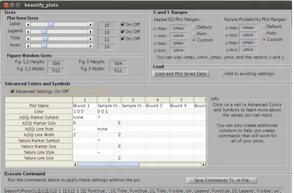
bound on kappa SQ (line) that holds with probability 1 . . . 62 Figure 4.2 In this plot we show the failure rate of a numerical experiment on kappa SQ. 62 Figure 4.3 kappaSQ GUI with advanced features shown. . . 64 Figure 4.4 Beautify Plots GUI. . . 64 Figure 4.5 The solid line shows Bound 1 and the triangles show the results of the

(13)

Chapter 1

Introduction

The leverage scores of am⇥nmatrixA with full column rank are defined as follows:

`i(A) =keTi Qk22, for 1im,

where Q is any basis of orthonormal columns for the column space of A. Conceptually, the leverage scores give a “measure” of the relative importance of each row where the meaning of the word ‘importance’ depends on the application. They were first described in [20] where the authors used leverage scores as a regression diagnostic for least squares to help identify potential outliers in the data. In the paper, they describe how the magnitude of the ith leverage score gives a measure of the influence of the ith _{row on the least squares fit. If the} _ith _{leverage score} is large, and one questions the accuracy of the corresponding data point, then one may want to remove the data point in order to better fit the rest of the data. Leverage scores are also used in importance sampling for low rank matrix approximation. In [26, 14, 31], leverage scores are used to identify important rows and columns 1 which are then used (or sampled with higher probability) to approximate the matrix. Leverage scores have also been used in the following [25, 13, 14, 6, 35, 12, 7].

In Chapter 2, motivated by the least squares solver Blendenpik[1], we investigate three strategies for uniform sampling of rows from matricesQwith orthonormal columns. The goal is to determine, with high probability, how many rows are required so that the sampled matrices have full rank and are well-conditioned with respect to inversion. Extensive numerical exper-iments illustrate that the three sampling strategies (without replacement, with replacement, and Bernoulli sampling) behave almost identically, for small to moderate amounts of sampling. In particular, sampled matrices of full rank tend to have two-norm condition numbers of at

1_{There are more general definitions of leverage scores than what we examine in this dissertation. Leverage}

(14)

most 10.

We derive a bound on the condition number of the sampled matrices in terms of the coher-enceµof Qwhere the coherence is simply the largest leverage score. This bound applies to all three di↵erent sampling strategies; it implies a, not necessarily tight, lower bound of_O(mµlnn) for the number of sampled rows; and it is realistic and informative even for matrices of small dimension and the stringent requirement of a 99 percent success probability.

For uniform sampling with replacement we derive a potentially tighter condition number bound in terms of the leverage scores of Q. To obtain a more easily computable version of this bound, in terms of just the largest leverage scores, we first derive a general bound on the two-norm of diagonally scaled matrices.

To facilitate the numerical experiments and test the tightness of the bounds, we present deterministic algorithms to generate matrices with user-specified coherence and leverage scores. In Chapter 3, we derive bounds for the leverage scores as well as leverage scores computed from the top k left singular vectors. Our bounds show that if the principal angles between A and B are small, then the leverage scores of B are close to the leverage scores of A. Next, we use two results by Wedin [41, 40] to bound the principal angles from above in terms of the singular values of A and kB Ak2. Finally, we combine these results and derive bounds for the leverage scores of B in terms of the singular values of A and _kB A_k2 and show that if kB A_k2 and n(A) 1 are small, then the leverage scores of B are close to the leverage scores of A. Additionally, we show that if kB Ak2 is small with respect to the kth singular value gap, then the leverage scores ofAand B, as computed from the topkleft singular vectors, are close.

(15)

Chapter 2

The E

↵

ect of Coherence on

Sampling From Matrices With

Orthonormal Columns, and

Preconditioned Least Squares

Problems

2.1 Introduction

This chapter was inspired by Avron, Maymounkov and Toledo’s Blendenpik algorithm and analysis [1].

Blendenpik is an iterative method for solving overdetermined least squares/regression prob-lems minxkAx bk2 with the Krylov space method LSQR [30]. In order to accelerate conver-gence, Blendenpik constructs a preconditioner Rs and solves instead the preconditioned least squares problem minzkAR_s1z bk2. The solution to the original problem is recovered by solv-ing a linear system with coefficient matrixRs. The innovative feature is the construction of the preconditionerRs by a random sampling method.

2.1.1 Motivation

(16)

Here is a conceptual point of view of how Blendenpik constructs the preconditioner: First it “smoothes out” the rows of A by applying a randomized unitary transform F, and then it uniformly samples (i.e. selects) a small number of rows Ms fromF A. At last it computes a QR factorization of the smaller sampled matrix,Ms=QsRs, where the triangular factor Rs serves as the preconditioner.

The neat and crucial observation in [1] is to realize that sampling rows from F A amounts, conceptually, to sampling rows from an orthonormal basis of F A. That is, if the columns of Q represent an orthonormal basis for the column space of F A, and if S is a sampling matrix thenSQhas the same two-norm condition number as AR 1

s . This means, it suffices to consider sampling from matricesQ with orthonormal columns.

The analysis in [1] suggests that SQ is well conditioned, if Q has low “coherence”. Intu-itively, coherence gives information about the localization or “uniformity” of the elements of Q. Mathematically, coherence is the largest (squared) norm of any row ofQ. For instance, ifQ consists of canonical vectors, then the non-zero elements are concentrated in only a few rows, so that Q has high coherence. However, if Q is a submatrix of a Hadamard matrix, then all elements have the same magnitude, so that Qhas low coherence.

If Q has low coherence, then, in the context of sampling, all rows are equally important. Hence any sampled matrix SQ with sufficiently many rows is likely to have full rank. The purpose of the randomized transformF is to produce a matrix F Awhose orthonormal basisQ has low coherence.

We were intrigued by the analysis ofBlendenpik because it appears to be the first to exploit the concept of coherence for numerical purposes. We also wanted to get a better understanding of the condition number bound for SQ in [1, Theorem 3.2], which contains an unspecified constant, and of the e↵ect of uniform sampling strategies.

2.1.2 Overview and main results

We survey the contents of the chapter , with a focus on the main results.

From preconditioned matrices to sampled matrices with orthonormal columns (Sec-tion 2.2)

(17)

the same two-norm condition number1_,

(AR_s1) =(SQ).

Then we discuss the notion of coherence and its properties (Section 2.2.2). For am_⇥nmatrix Qwith orthonormal columns, QTQ=In, thecoherence

µ⌘ max 1jmke

T jQk22

is the largest squared row norm2_.

Sampling methods (Section 2.3)

We discuss three randomized methods for producing sampling matrices S: Sampling without replacement (Section 2.3.1), sampling with replacement (Section 2.3.2), and Bernoulli sampling (Section 2.3.3). We show that Bernoulli sampling can be viewed as a form of sampling without replacement (Section 2.3.4).

The sampling matricesSfrom all three methods are constructed so thatSTSis an unbiased estimator of the identity matrix. The action of applying S to a matrix Q with orthonormal columns,SQ, amounts to randomly sampling rows from Q.

The numerical experiments (Section 2.3.5) illustrate two points: First, the three sampling methods behave almost identically, in terms of the percentage of sampled matricesSQthat have full rank and their condition numbers, in particular for small to moderate sampling amounts. Second, those sampled matricesSQ that have full rank tend to be very well-conditioned, with condition numbers (SQ)_10.

As a consequence (Section 2.3.6), we recommend sampling with replacement forBlendenpik, because it is fast, and it is easy to implement.

Numerical experiments

Since random sampling methods can be expected to work well in the asymptotic regime of very large matrix dimensions, we restrict all numerical experiments to matrices of small dimension. Furthermore, we consider only matrices that have many more rows than columns, m n. This is the situation where random sampling methods can be most efficient. In contrast, random sampling methods are not efficient for matrices that are almost square, because the number of rows inSQhas to be at least equal to n, otherwise rank(SQ) =nis not possible.

1_Here_₍_X₎

⌘ kXk2kX†k2 denotes the Euclidean two-norm condition number with respect to inversion of a

full rank matrixX. The matrixX†_{is the Moore-Penrose inverse of}_X_.

2_{The superscript}_T _{denotes transpose, and}_I

(18)

Condition number bounds based on coherence (Section 2.4)

We derive a probabilistic bound, in terms of coherence, for the condition numbers of the sampled matrices (Theorem 7 in Section 2.4.1). The bound applies to all three sampling methods. From this we derive the following lower bound, not necessarily tight, on the required number of sampled rows.

Preview of Corollary 8 Given a failure probability0< <1, and a tolerance0✏<1.

To achieve the condition number bound (SQ) _q1+₁ ✏_✏, the number of rows from Q, sampled by any of three methods, should be at least

c 3mµ ln(2n/ )

✏2 . (2.1)

This suggests that one has to sample more rows for SQ if Q has high coherence (µ close to 1), if one wants a low condition number bound (small ✏), or if one wants a high success probability (small ).

Numerical experiments (Section 2.4.2) illustrate that the bounds are informative for matrices with sufficiently low coherenceµ and sufficiently high aspect ratio m/n. Our bounds have the following advantages (Section 2.4.3):

1. They are tighter than those in [1, Theorem 3.2] because they are non-asymptotic, with all constants explicitly specified.

2. They apply to three di↵erent sampling methods.

3. They imply a lower bound, of⌦(mµlnn), on the required number of sampled rows. 4. They are realistic and informative – even for matrices of small dimension and the stringent

requirement of a 99 percent success probability.

Condition number bounds based on leverage scores, for uniform sampling with replacement (Section 2.5)

The goal is to tighten the coherence-based bounds from Section 2.4 by making use of all the row norms of Q, instead of just the largest one. To this end we introduce leverage scores (Section 2.5.1), which are the squared row norms of Q,

`j =keTjQk22, 1jm.

(19)

largest leverage scores (Section 2.5.3). It implies the following lower bound, not necessarily tight, on the number of samples.

Preview of Corollary 15 Given a failure probability 0 < < 1, a tolerance 0 _✏< 1,

and a labeling of leverage scores in non-increasing order,

µ=`[1] · · · `[m].

To achieve the condition number bound (SQ) _q1+₁ ✏_✏, the number of rows from Q, sampled uniformly with replacement, should be at least

c 2₃m(3⌧ +✏µ) ln(2n/ )

✏2 , (2.2)

where t_{⌘ b}1/µ_c and⌧ _⌘µ Pt_j=1`_[j]+ (1 t µ)`_[t+1].

We show (Section 2.5.4) that (2.2) is indeed tighter than (2.1). This is confirmed by nu-merical experiments (Section 2.5.5). The di↵erence becomes more drastic for matrices Q with widely varying non-zero leverage scores, and can be as high as ten percent. Hence (Section 2.5.6), when it comes to lower bounds for the number of rows sampled uniformly with replacement, we recommend (2.2) over (2.1).

Algorithms for generating matrices with prescribed coherence and leverage scores (Section 2.6)

The purpose is to make it easy to investigate the efficiency of the sampling methods in Sec-tion 2.3, and test the tightness of the bounds in SecSec-tions 2.4 and 2.5.

To this end we present algorithms for generating matrices with prescribed leverage scores and coherence (Section 2.6.1), and for generating particular leverage score distributions with prescribed coherence (Section 2.6.2). Furthermore we present two classes of structured matrices with prescribed coherence that are easy and fast to generate (Section 2.6.3). The basis for the algorithms is the following majorization result.

Preview of Theorem 25 Given integersm nand a vector`withm elements that satisfy

0`j 1 andPm_j=1`j =n, there exists a m⇥nmatrixQ with orthonormal columns that has leverage scores _keT

jQk22=`j, 1jm, and coherenceµ= max1jm`j.

Bound for two-norms of diagonally scaled matrices (Section 2.8)

(20)

Preview of Theorem 22 Let Z be a m_⇥n matrix with rank(Z) =n and largest squared row norm µz ⌘ max1jmkeTjZk22. Let D be a m⇥m non-negative diagonal matrix, and a labeling of diagonal elements in non-increasing order,

kD_k2 =d_[1] _{· · ·} d_[m] 0.

If t⌘⌅(kZ†k2 2µz) 1

⇧

, then either

kDZ_k2₂ _µz t

X

j=1

d2_[j]+ _kZ_k2₂ t µz d2[t+1] ifkZk22 t µzµz

or

kDZk22µz t+1

X

j=2

d2_[j]+ kZk22 t µz d2[1]. if kZk22 t µz > µz.

Proofs (Sections 2.7, 2.8 and 2.9)

All proofs, except those for Sections 2.2 and 2.3, have been relegated to these three sections. Section 2.7 contains the proofs for Sections 2.4 and 2.5, which are based on two matrix con-centration inequalities: A Cherno↵bound (Section 2.7.1), and a Bernstein bound (Section 2.7.4). Section 2.8 contains the proofs for the easily computable bounds in Sections 2.5.3 and 2.5.4, together with the majorization results (Section 2.8.1) required for the proofs.

The majorization results in Section 2.9 represent the foundation for the algorithms in Sec-tion 2.6.

2.1.3 Literature

Existing randomized least squares methods are based on randomized projections. This means, conceptually they multiplyA by a random matrix F, and then sample a few rows from F A.

The algorithms in [4, 12, 15] solve a smaller sampled problem by a direct method. Like

Blendenpik [1], the algorithm in [33] computes a preconditioner from the QR factorization of a sampled submatrix, but then solves the preconditioned problem by applying the conjugate gradient method to the normal equations. The parallel solver LSRN [27] computes a precon-ditioner from the SVD of a sampled submatrix, and then solves the preconditioned problem with an iterative method. This solver applies to general matrices rather than just those of full column rank.

(21)

2.1.4 Notation

The norm _k_·_k2 denotes the Euclidean two-norm, and the two-norm condition number with respect to inversion of a realm_⇥nmatrixZ with rank(Z) =nis denoted by(Z)_{⌘ k}Z_k2kZ†_k2, where Z† is the Moore-Penrose inverse. Thek⇥k identity matrix is Ik =

⇣

e1 . . . ek

⌘

, and its columns are thecanonical vectors ej, 1jk.

The probability of an event _X is denoted by Pr[_X], and the expected value of a random variableX is denoted byE[X].

2.2 The Blendenpik algorithm, and coherence

We describe the Blendenpik algorithm for solving least squares problems (Section 2.2.1), and present the notion of coherence (Section 2.2.2).

2.2.1 Algorithm

TheBlendenpik algorithm [1, Algorithm 1] solves full column rank least squares problems with the Krylov space methodLSQR[30] and a randomized preconditioner. Algorithm 2.2.1 presents a conceptual sketch of Blendenpik. The subscript “s” denotes quantities associated with the sampled matrix.

Algorithm 2.2.1 Sketch of Blendenpik [1]

Input: m⇥nmatrixA withm n and rank(A) =n,m⇥1 vectorb m⇥m random unitary matrixF

k_⇥nsampling matrixS withk n

Output: Solution of minxkAx bk2 M =F A _{Improve coherence_}

Ms=SM {Sample for preconditioner}

Thin QR factorization Ms=QsRs {Generate preconditioner}

Determine solution y to minzkARs1z bk2 {Solve preconditioned problem} Solve Rsxˆ=y {Recover solution to original problem}

(22)

The sampling matrix S selects k n rows from the transformed matrix M. We discuss di↵erent types of sampling matrices in Section 2.3. The k⇥n sampled matrix Ms has a thin QR decomposition Ms =QsRs where Qs is k⇥n with orthonormal columns and Rs is n⇥n upper triangular.

The basis for the analysis is the thin QR decomposition M =QR, where Qis m⇥nwith orthonormal columns andRisn_⇥nupper triangular. This QR decomposition isnotcomputed. The next result links the condition number of the preconditioned matrix to that of the matrix SQ, see also [1, Section 3.1] and [33, Theorem 1].

Lemma 1 With the notation in Algorithm 2.2.1, if rank(Ms) =n, then

(AR_s1) =(SQ).

Proof. From F A=M =QR and the fact that the 2-norm is invariant under premultiplica-tion by matrices with orthonormal columns, it follows that

(AR_s1) = (M R_s1) =(RR_s1) =(RsR 1) =(MsR 1) =(SM R 1) = (SQ).

In Sections 2.4 and 2.5 we derive bounds for the condition number of the preconditioned matrix,(AR_s1). Our bounds are tighter than those in [1, Theorem 3.2], because they have all constants explicitly specified, and apply to three di↵erent sampling strategies. Since Lemma 1 implies (AR 1

s ) = (SQ), we state the bounds for (SQ) only. An important ingredient in these bounds is the coherence of Q.

2.2.2 Coherence

Coherence gives information about the localization or “uniformity” of the elements in an or-thonormal basis. The more general concept ofmutual coherencebetween two orthonormal bases was introduced in [10, §VII], in the context of signal processing and computational harmonic analysis, to describe a condition for the existence of sparse representations of signals. What we use here is a special case, and can be viewed as a measure for how close an orthonormal basis is to sharing a vector with a canonical basis.

Definition 2 (Definition 3.1 in [1], Definition 1.2 in [7]) Let Q be a real m_⇥n matrix with orthonormal columns,QTQ=In, then thecoherence of Q is

µ_⌘ max 1jmke

(23)

If the columns of Q are an orthonormal basis for the column space of a matrixM, then the coherence of M isµ.

The second part of Definition 41 emphasizes that coherence is really a property of the column space, hence basis-independent. In other words, if ˆQ = QV, where V is a real n_⇥n orthogonal matrix, then ˆQand Q have the same coherence.

The range for coherence is _mn _µ_1. If Qis am_⇥nsubmatrix of the m_⇥m Hadamard matrix, thenµ=n/m. If a column ofQis a canonical vector, thenµ= 1. Hence an orthonormal basis has high coherence if it shares a vector with a canonical basis.

There are other definitions of coherence that di↵er from the above by factors depending on the matrix dimensions [32, Definition 1], [35, Definition 1]. However, the notion of statistical coherence in Bayesian analysis [24] appears to be unrelated.

2.3 Sampling Methods

We present three di↵erent types of sampling methods: Sampling without replacement (Sec-tion 2.3.1), sampling with replacement (Sec(Sec-tion 2.3.2), and Bernoulli sampling (Sec(Sec-tion 2.3.3). We show that Bernoulli sampling can be viewed as a form of sampling without replacement (Section 2.3.4). The numerical experiments illustrate that there is little di↵erence among the three methods for small to moderate amounts of sampling (Section 2.3.5). Hence we recommend sampling with replacement for Algorithm 2.2.1 (Section 2.3.6).

The sampling matricesSin all three methods are scaled so thatSTSis an unbiased estimator of the identity matrix.

2.3.1 Sampling without replacement

The obvious sampling strategy, in Algorithm 2.3.1, picks the requested number of rows, so that the sampling matrix S is just a scaled submatrix of a permutation matrix.

Uniform sampling without replacement can be implemented via random permutations3_{. A} permutation ⇡1, . . . ,⇡m of the integers 1, . . . , mis a random permutation, if it is equally likely to be one of m! possible permutations [29, pages 41 and 48].

The following lemma presents the probability that sampling without replacement picks a particular row.

Lemma 3 If Algorithm 2.3.1 samples c out of m indices, then the probability that a particular index is picked equals c/m.

(24)

Algorithm 2.3.1 Uniform sampling without replacement [16, 18]

Input: Integers m 1 and 1_c_m

Output: c⇥msampling matrix S with E[STS] =Im Let k1, . . . , km be a random permutation of 1, . . . , m S =pm_c ek1 . . . ekc

T

Proof. The probability that some index, sayr, is not sampled in the first trial is 1 _m1 = m_m1. Now there are onlym 1 indices left. So the probability that indexris not sampled in the second trial is 1 _m1₁ = m_m 2₁. Repeating this argument shows that with probabilityQc_t=1_{m t+1}m t = m c_m indexr is not sampled in ctrials.

The complementary event, the probability that index r is sampled, equals 1 m c_m = _mc.

2.3.2 Sampling with replacement

This is the sampling strategy that appears to be analyzed in [1]. It samples exactly the requested number of rows, but with replacement, which means a row may be sampled more than once. Algorithm 2.3.2 is the same as the EXACTLY(c) algorithm [15, Algorithm 3] with uniform probabilities, which is also used in theBasicMatrixMultiplication Algorithm [11, Fig. 2].

Algorithm 2.3.2 Uniform sampling with replacement [11, 15]

Input: Integers m 1 and 1_c_m

Output: c⇥msampling matrix S with E[STS] =Im

for t= 1 :c do

Samplektfrom {1, . . . , m} with probability 1/m, independently and with replacement

end for

S =pm_c ek1 . . . ekc

T

Sampling with replacement (Algorithm 2.3.2) is often easier to analyze and implement than sampling without replacement (Algorithm 2.3.1), and it can also be more robust to errors [29,

(25)

2.3.3 Bernoulli sampling

The sampling strategy in Algorithm 2.3.3 is implemented inBlendenpik [1, Algorithm 1]. Fol-lowing [18, Section A], we use the term Bernoulli sampling, because the strategy treats each row as an independent, identically distributed Bernoulli random variable. Each row is either sampled or not, with the same probability for each row. Algorithm 2.3.3 produces a m_⇥m square matrix S – in contrast to Algorithms 2.3.1 and 2.3.2, which produce c_⇥m matrices.

Algorithm 2.3.3 Bernoulli sampling [1, 16, 18]

Input: Integers m 1 and 1cm

Output: m_⇥m sampling matrixS withE[STS] =Im S = 0m_⇥m

for t= 1 :m do

Stt=pm_c

(

1 with probability _mc 0 with probability 1 _mc

end for

The number of sampled rows, which is equal to the number of non-zero diagonal elements in S, is not known a priori, but the expected number of sampled rows isc. The lemma below shows that the actual number of rows picked by Bernoulli sampling is characterized by a binomial distribution [34, Section 2.2.2].

Lemma 4 If Algorithm 2.3.3 samples from m indices with probability _⌘c/m, then the prob-ability that it picks exactly kindices equals m_k k(1 )m k.

Proof. Determining the diagonal elements of them⇥msampling matrixSin Algorithm 2.3.3 can be viewed as performing m independent trials, where trial t is a success (Stt 6= 0) with probability , and a failure (Stt = 0) with probability 1 . The probability of k successes is given by the binomial distribution m_k k(1 )m k.

2.3.4 Relating Bernoulli sampling and sampling without replacement

We show that Bernoulli sampling (Algorithm 2.3.3) is the same as first determining the number of samples with a binomial distribution (motivated by Lemma 4), and then sampling without replacement (Algorithm 2.3.1). This is described in Algorithm 2.3.4 below.

(26)

Algorithm 2.3.4 Simulating Algorithm 2.3.3 with Algorithm 2.3.1

Input: Integers m 1 and 1cm

Output: ˜c_⇥msampling matrix S with E[STS] =Im

that “behaves like” a sampling matrix generated by Algorithm 2.3.3 ⌘c/m

Sample ˜cfrom {1, . . . , m} wherePr[˜c=k] = m_k k(1 )m k

Use Algorithm 2.3.1 to sample ˜c indicesk1, . . . , k˜c uniformly and without replacement S =pm_˜_c ek1 . . . ek˜c

T

Lemma 5 The probability that Algorithm 2.3.4 picks a particular index equals =c/m. Proof. Motivated by Lemma 4, the actual number of samples k in Algorithm 2.3.4 is given by a binomial distribution. Once a specific k has emerged, one applies Lemma 3 to conclude that the probability that Algorithm 2.3.1 picks some index r isk/m.

Now the probability that Algorithm 2.3.4 picks some index r is obtained by conditioning [34, Section 3.5] on the number of samples, k, and equals

m

X

k=0

Pr[k indices sampled] Pr[index r sampled|k indices sampled]

= m

X

k=1

✓

m k

◆

k ₍₁ ₎m k k m

=

m_X1

k=0

✓

m 1

k

◆

k₍₁ ₎m 1 k₌ _{( + (1} ₎₎m 1 ₌ _,

where the first equality follows from the zero summand fork= 0.

Finally, we can conclude that sampling with Algorithm 2.3.4 is the same as sampling with Algorithm 2.3.3.

Theorem 6 Both, Algorithms 2.3.4 and 2.3.3 pick a particular set of indices i1, . . . , ic with probability c(1 )m c.

(27)

that Algorithm 2.3.4 picks indices i1, . . . , ic equals 1

m c

✓

m c

◆

c₍₁ ₎m c₌ c₍₁ ₎m c_.

2.3.5 Numerical experiments

We present two representative comparisons of the three sampling strategies, with two plots for each strategy: The condition numbers of full-rank sampled matrices SQ, and the failure percentage, that is the percentage of sampled matrices SQthat are numerically rank deficient (as determined by the Matlab commandrank).

The experiments are limited to very tall and skinny matrices (with many more rows than columns,m n), because that’s when the sampling strategies are most efficient. In particular, sincec nis required forSQto have full column rank, sampling methods are inefficient when nis not much smaller than m, in which case a deterministic algorithm would be preferable.

Experimental setup

The m⇥n matrices Q with orthonormal columns have m = 104 rows and n = 5 columns. The condition numbers and failure percentages are plotted against various sampling amounts c, with 30 runs for eachc. For the failure percentages we display only those sampling amounts c that give rise to rank-deficient matrices, in these particular 30 runs. For Algorithm 2.3.3 the horizontal axis represents the numerator c in the probability, that is, the expected number of sampled rows. All three strategies sample from the same matrix.

We consider two di↵erent types of matrices: Matrices with low coherence µ = 1.5n/m in Figure 2.1; and matrices with higher coherenceµ= 150n/m and many zero rows in Figure 2.2. Our numerical experiments indicate that these coherence values are representative, in the sense that di↵erent values of coherence would not produce any other interesting e↵ects.

Figure 2.1

(28)

250 500 750 1000 1 2 5 10 c κ (SQ)

5 10 15 21

0 25 50 75 100 c

% of rank deficient SQ

(a) Algorithm 2.3.1: Sampling without replacement

250 500 750 1000

1 2 5 10 c κ (SQ)

5 10 20 30 35

0 25 50 75 100 c

(b) Algorithm 2.3.2: Sampling with replacement

250 500 750 1000

1 2 5 10 c κ (SQ)

5 10 20 30 40 46

0 25 50 75 100 c

(c) Algorithm 2.3.3: Bernoulli sampling

(29)

40001 5000 6000 7000 8000 9000 10000 2 5 10 c κ (SQ)

40000 4500 5000 5222

1 3 5 7 10 c

(a) Algorithm 2.3.1: Sampling without replacement

40001 5000 6000 7000 8000 9000 10000 2 5 10 c κ (SQ)

40000 4500 5000 5500 6000 6500 7000 7500 7732 1 3 5 7 10 c

(b) Algorithm 2.3.2: Sampling with replacement

40001 5000 6000 7000 8000 9000 10000

2 5 10 c κ (SQ)

40000 4500 5000 5301

1 3 5 7 10 c

(c) Algorithm 2.3.3: Bernoulli sampling

(30)

Figure 2.2

Shown are condition numbers and percentage of rank deficient matrices for a matrix Q, gener-ated by Algorithm 2.6.3, with coherence 150n/m and many zero rows. The number of sampled rows ranges from c = 4000 to m. The sampled matrices SQ of full rank are very well condi-tioned, with (SQ) _ 10. Even for c = 4,000, as many 10 percent of the sampled matrices can still be rank-deficient. All three algorithms have to sample more than half of the rows ofQ in order to always produce matrices SQwith full column rank. Specifically in these particular runs, Algorithms 2.3.1 and 2.3.3 need to sample c 5,222 and c 5,301 rows, respectively, while Algorithm 2.3.1 needsc 7732.

Note that the condition numbers of matrices from Algorithms 2.3.1 and 2.3.3 approach 1 as more and more rows are sampled. This is because no row is sampled more than once; and for c=m all rows are sampled.

Again, the three strategies exhibit almost identical behavior: The sampled matrices SQ of full rank are very well conditioned, with (SQ) _ 10. However, due to the higher coherence, numerically rank-deficient matrices occur more frequently.

2.3.6 Conclusions for Section 2.3

The numerical experiments illustrate that the three sampling strategies behave almost identi-cally, in particular for small to moderate sampling amounts, and that sampled matrices of full rank tend to be very well-conditioned4. Furthermore, Section 2.3.4 shows that Bernoulli sam-pling can be viewed as a form of samsam-pling without replacement, and the numerical experiments confirm the similarity in behavior.

Among the three strategies, we recommend sampling with replacement (Algorithm 2.3.2) for small to moderate amounts of sampling in Algorithm 2.2.1. It is fast and easy to implement in both.

2.4 Condition number bounds based on coherence

We derive bounds for the condition numbers of matrices produced by the sampling strategies in section 2.3, in terms of coherence. These bounds are based on a specific concentration inequality and imply a, not necessarily tight, lower bound for the number of sampled rows (Section 2.4.1). Numerical experiments illustrate that the bounds are informative (Section 2.4.2). We end this section by summarizing the main features of the bounds (Section 2.4.3).

(31)

2.4.1 Bounds

We show that the three sampling strategies in Section 2.3 all have the same condition number bound, in terms of coherence.

Theorem 7 below is based on a matrix Cherno↵ concentration inequality (Section 2.7.1). We chose this particular inequality because extensive numerical experiments with our Matlab toolboxkappaSQ v3[22] suggest that it tends to produce the tightest bound.

Theorem 7 Let Q be a real m ⇥n matrix with QTQ = In and coherence µ. Let S be a sampling matrix produced by Algorithms 2.3.1, 2.3.2, or 2.3.3 with ncm. For 0<✏<1 and f(x)_⌘ex_{(1 +}_x) (1+x) _define

⌘n⇣f( ✏)c/(mµ)+f(✏)c/(mµ)⌘.

If <1, then with probability at least 1 we have rank(SQ) =n and

(SQ)_

r

1 +✏ 1 ✏.

Proof. The proof is based on results from [16, 36, 37] and is relegated to Section 2.7.2. Since 0 < f(_±✏) < 1 for 0 < ✏ < 1, Theorem 7 implies that the sampling strategies in Section 2.3 are more likely to produce full-rank matrices as the number c of sampled rows increases. Furthermore, for a given total number of rowsm, matrices Q with fewer columnsn and lower coherence µare more likely to give rise to sampled matricesSQ that have full rank. Theorem 7 implies the following lower bound on the number of samples, but we make no claims about the tightness of this bound.

Corollary 8 Under the assumptions of Theorem 8,

c 3mµ ln(2n/ ) ✏2

samples are sufficient to achieve (SQ)q1+✏

1 ✏ with probability at least 1 .

Proof. See Section 2.7.3.

Corollary 8 implies that the sampling strategies in Section 2.3 should sample at least c= ⌦(mµlnn) rows to produce a full rank, well-conditioned matrix. In particular, ifQhas minimal coherence µ = n/m, then Corollary 8 implies that the number of sampled rows should be at least

c 3nln(2n/ )

(32)

that is c=⌦(nlnn).

To achieve (SQ) 10 with probability at least .99 requires that the number of sampled rows be at least

c 3.2mµ (ln(2n) + 4.7). (2.4)

Here we chose✏0= 99/101, so that the condition number bound equals q1+✏0

1 ✏0 = 10.

Remark 9 Theorem 7 is informative only for sufficiently low coherence values.

For instance, consider the higher coherence matrices from Figure 2.2 in Section 2.3.5 with m= 10,000, n= 5 and coherenceµ= 150n/m. Choose ✏= 99/101so that (SQ)10, and a failure probability =.01. Then Corollary 8 implies the lower bound c 12,408, which means that the number of sampled rows would have to be larger than the total number of rows.

2.4.2 Numerical experiments

We compare the bound for the condition numbers of the sampled matrices (Theorem 7) with the true condition numbers of matrices produced by sampling with replacement (Algorithm 2.3.2). There are several reasons why it suffices to consider only a single sampling strategy: The three sampling methods all have the same bound (Theorem 7); Bernoulli sampling is a form of sampling without replacement (Section 2.3.4); and all three sampling methods exhibit very similar behavior for matrices of low coherence (Sections 2.3.5 and 2.3.6). Furthermore, this allows a clean comparison with the bounds in Section 2.5 which apply only to Algorithm 2.3.2.

Experimental setup

The m_⇥n matrices Q with orthonormal columns have m = 104 rows and n = 5 columns. The left panels in Figure 2.3 show the condition numbers of the full-rank sampled matricesSQ produced by Algorithm 2.3.2 against di↵erent sampling amountsc, with 30 runs for eachc. The right panels in Figure 2.3 show the percentage of rank deficient matrices SQ against di↵erent sampling amounts c. We display only those sampling amountsc that give rise to rank-deficient matrices, in these particular 30 runs.

The left panels in Figure 2.3 also show the condition number bound ✏ ⌘

q

1+✏

1 ✏ from

Theorem 7. For each value ofc, we obtain✏as the solution of the nonlinear equationFc(x)2 = 0 associated with Theorem 7 and defined as

Fc(x)⌘ n

⇣

f( x)c/(mµ)+f(x)c/(mµ)⌘.

(33)

probabil-ity. Since an explicit expression seems out of reach, we use unconstrained nonlinear optimization (a Nelder-Mead simplex direct search) to solveFc(x)2 = 0. This is done in Matlab with a code equivalent to

✏= fminsearch(Fc(x)2,0,10 30) ,

where fminsearch starts at the point 0, and terminates when |Fc(✏)|2 _ ₁₀ 30_{. If 0} _<_✏ _< ₁ then✏ is plotted, otherwise nothing is plotted.

As explained in Remark 9, Theorem 7 is not informative for higher coherence values, so we consider matrices with the following properties: Minimal coherence µ=n/m in Figure 2.3(a); low coherence µ= 1.5n/m in Figure 2.3(b); slightly higher coherence µ = 15n/m with many zero rows in Figure 2.3(c). The matrices for Figures 2.3(a) and 2.3(b) were generated with Algorithm 2.6.2, while the matrix for Figure 2.3(c) was generated with Algorithm 2.6.3.

Figure 2.3

The left panels illustrate that Theorem 7, constrained to a 99 percent success probability, correctly predicts the magnitude of the condition numbers, i.e. (SQ)10. Hence Theorem 7 provides informative qualitative bounds for matrices with very low coherence, as well as for matrices with slightly higher coherence and many zero rows.

Table 2.1

This is a comparison of the numerical experiments in Figure 2.3 with the bounds from Theorem 7 and Corollary 8, both restricted to a 99 percent success probability.

The third column depicts the highest values of c for which a rank-deficient matrix occurs, during these particular 30 runs. It should be kept in mind that these values are highly dependent on the particular sampling runs. This column is to be compared to the fourth column which contains the lowest values of c where Theorem 7 starts to apply. Although there is a gap between the occurrence of the last rank deficiency and the onset of Theorem 7, the values have qualitatively the same order of magnitude.

The rightmost column in Table 2.1 contains the values of the lower bound (2.4), and is to be compared to the column with the starting values for Theorem 7. Although (2.4) is weaker than Theorem 7, its values are close to the starting values of Theorem 7, especially for lower co-herence. Hence, the lower bound (2.4) captures the correct magnitude of the sampling amounts where Theorem starts to become informative.

(34)

5 500 1000 1 2 5 10 c κ (SQ)

5 10 20 30 31

0 25 50 75 100 c

(a)Qhas minimal coherenceµ=n/m. Sampling amounts aren_c_1,000.

250 500 750 1000 1 2 5 10 c κ (SQ)

5 10 15 20 25 31

0 25 50 75 100 c

(b)Qhas low coherenceµ= 1.5n/m. Sampling amounts arenc1,000.

43 1000 2000 3000

1 2 5 10 c κ (SQ)

5 100 200 300 400 500 600 700 740 0 25 50 75 100 c

(c)Qhas slightly higher coherenceµ= 15n/mand many zero rows. Sampling sampling amounts are

n_c_3,000.

(35)

Table 2.1: Comparison of information from Figure 2.3, with Theorem 7 and Corollary 8.

Figure coherence µ last rank deficiency Theorem 7 (2.4) occurs at c= starts atc=

2.3(a) n/m 31 81 83

2.3(b) 1.5n/m 31 121 125

2.3(c) 15n/m 740 1207 1241

The bounds in Theorem 7 and Corollary 8 have the following advantages:

1. They are non-asymptotic bounds, where all constants have explicit numerical values, hence they are tighter than the bounds in [1, Theorem 3.2].

2. They apply to three di↵erent sampling methods.

3. They imply a lower bound, of ⌦(mµlnn), on the required number of sampled rows. Although we did not give a formal proof of tightness, numerical experiments illustrate that sampling only the required number of rows implied by the bound is realistic. numerical experiments illustrate that the bound is realistic.

4. Even under the stringent requirement of a 99 percent success probability, they are infor-mative for matrices of small dimension because they correctly predict the magnitude of the condition numbers for the sampled matrices.

Note that the bounds in Theorem 7 and Corollary 8 are informative only for matrices that are tall and skinny (m n) and have low coherence. The restriction to tall and skinny matrices is not an imposition, because it is required for the e↵ectiveness of the sampling strategies, see Section 2.3.5.

In the next section we try to relax the restriction to low coherence matrices, by more thoroughly exploiting the information available from the row norms ofQ.

2.5 Condition number bounds based on leverage scores, for

uni-form sampling with replacement

(36)

row norms of Q. We use them to derive a bound for uniform sampling with replacement (Sec-tion 2.5.2), and for more easily computable versions of the bound (Sec(Sec-tion 2.5.3). Analytical (Section 2.5.4) and experimental (Section 2.5.5) comparisons demonstrate that the implied lower bound on the number of sampled rows is better than the coherence-based bounds in Section 2.4. A review with some reflection ends this section (Section 2.5.6).

2.5.1 Leverage scores

So-calledstatistical leverage scores were first introduced in 1978 by Hoaglin and Welsch [20] to detect outliers when computing regression diagnostics, see also [8, 38]. Mahoney and Drineas pioneered the use of leverage scores for importance sampling strategies in randomized matrix computations [25].

Specifically, if M is a real m⇥n matrix with rank(M) =n, then them⇥m hat matrix

H _⌘M(MTM) 1MT

is the orthogonal projector onto the column space of M, and its diagonal elements are called leverage scores [20, Section 2]. Hence, leverage scores are basis-independent. For our purposes, though, it suffices to define them in terms of a thin QR decomposition M = QR, so that the hat matrix can be expressed asH =QQT.

Definition 10 If Q is a m⇥n matrix with QTQ=In, then its leverage scores are

`j ⌘ keTjQk22, 1jm.

Them⇥m diagonal matrix of leverage scores is

L_⌘diag(`1, . . . ,`m).

Note that the coherence is the largest leverage score,

µ= max

1jm`j =kLk2. 2.5.2 Bounds

(37)

Theorem 11 Let Q be a m_⇥n real matrix with QT_Q ₌ _I

n, leverage scores `j, 1  j  m, and coherence µ. Let S be a sampling matrix produced by Algorithm 2.3.2 with ncm. For 0<✏<1 set

⌘2nexp

✓

3 2

c✏2

m(3kQT_LQ_k2₊_✏µ)

◆

.

If <1, then with probability at least 1 we have rank(SQ) =n and

(SQ)_

r

1 +✏ 1 ✏.

Proof. The proof uses results from [2, 32] and is relegated to Section 2.7.5.

Like Theorem 7, Theorem 11 implies that sampling with replacement is more likely to produce full-rank matrices as the numbercof sampled rows increases. Furthermore, for a given total number of rows m, matrices Q with fewer columns n and lower coherence µ are more likely to yield sampled matricesSQ that have full rank. The dependence of _kQT_LQ_k2 _on _µ _is discussed below.

Remark 12 The norm _kQT_LQ_k2 _{has simple and tight bounds in terms of the coherence,}

µ2_{ k}QTLQ_k2 _µ. (2.5)

The lower bound follows from kQTLQk2 =kL1/2Qk2 2 and

kL1/2Q_k2 _keT_jL1/2Q_k2 =`_j1/2_keT_jQ_k2 =`j, 1jm,

which implies kL1/2Qk2 µ.

The bounds (2.5) are attained for extreme values of the coherence:

• In case of minimal coherence µ = `j for all 1  j  m, we have L = µIm. Thus kQTLQk2 =µkQTQk2 =µ, and the upper bound is attained.

• In case of maximal coherence µ = 1, we have µ2 = µ. Thus kQTLQk2 = µ2 = µ, and both, lower and upper bounds are attained.

2.5.3 Computable bounds

We present easily computable bounds for kQTLQk2, based on coherence and several of the largest leverage scores.

To this end, we use a labeling of the leverage scores in non-increasing order,

(38)

Corollary 13 Under the assumptions of Theorem 11, ift_{⌘ b}1/µ_c, then

kQTLQ_k2 _µ t

X

j=1

`_[j]+ (1 t µ)`_[t+1]_µ.

If, in addition, t is an integer, then _kQTLQ_k2_µ Pt_j=1`_[j].

The number of large leverage scores appearing in Corollary 13 depends on the coherence: Few leverage scores for high coherence, but more for low coherence. Henceforth we will use the approximation from Corollary 13 instead of the true value kQTLQk2, for two reasons: First, numerical experiments show that the approximation tends to be very accurate. Second, the approximation is convenient, because it requires only a leverage score distribution rather than a full-fledged matrix Q.

Remark 14 Corollary 13 is tight for the extreme cases of minimal and maximal coherence.

• In case of minimal coherenceµ=`j for all1jm, Remark 12 implieskQTLQk2 =µ. The bound in Corollary 13 is _kQT_LQ_k2 __{µ, thus tight.}

• In case of maximal coherenceµ= 1, Remark 12 implies_kQT_LQ_k2 ₌_µ2 ₌_{µ. Corollary 13} holds witht= 1 and gives the bound_kQT_LQ_k2__{µ, which is tight as well.}

Inserting this approximation for kQTLQk2 into the expression for in Theorem 11 yields a, not necessarily tight, lower bound on the number of samples.

Corollary 15 Under the assumptions of Theorem 11,

c 2₃m(3⌧ +✏µ)ln(2n/ ) ✏2 ,

where ⌧ _⌘µ Pt_j=1`_[j]+ (1 t µ)`_[t+1], samples are sufficient to achieve (SQ) _q1+₁ ✏_✏ with probability at least 1 .

In particular, if Q has minimal coherence µ = n/m, then Corollary 15 implies that the number of sampled rows should be at least

c 3nln(2n/ ) ✏2 .

(39)

To achieve (SQ) _10 with probability at least .99 requires that the number of sampled rows be at least

c m(2.1⌧+.7µ) (ln(2n) + 4.7). (2.6)

2.5.4 Analytical comparison of the bounds in Sections 2.4.1 and 2.5.2 An analytical comparison between Theorems 7 and 11 is not obvious, because they are based on di↵erent concentration inequalities. Instead we compare the implied lower bounds for the number of sampled rows, and show that the leverage-score based bound in Corollary 15 is at least as tight as the coherence-based bound in Corollary 8.

Corollary 16 Under the assumptions of Theorem 11 and Corollary 13,

2

3m(3⌧+✏µ)

ln(2n/ )

✏2 3mµ

ln(2n/ ) ✏2 .

Hence Corollary 15 is at least as tight as Corollary 8.

2.5.5 Experimental comparison of the bounds in Sections 2.4.1 and 2.5.2 We present numerical experiments to compare the lower bounds for the number of sampled rows in Corollaries 8 and 15, for di↵erent values of coherence. This gives quantitative insight into the comparison in Corollary 16, and illustrates the reduction in the number of sampled rows from Corollary 15, as compared to Corollary 8.

Experimental setup

As in previous sections, we use m⇥n matrices with m = 104 rows and n= 5 columns. The success probability is .99; and ✏= 99/101, so that the bound for (SQ) is equal to 10. Hence the bounds in Corollaries 8 and 15 amount to (2.4) and (2.6), respectively.

We consider two di↵erent leverage scores distributions: A distribution generated by rithm 2.6.2 with one large leverage score in Table 2.2; and a distribution generated by Algo-rithm 2.6.3 with as many zeros as possible in Table 2.3.

Table 2.2

(40)

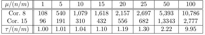
Table 2.2: Lower bounds for number of sampled rows in Corollaries 8 and 15 and approximation ⌧, for di↵erent values of coherence µ. The first value represents minimal coherence µ =n/m. Herem= 10,000,n= 5, =.01,✏= 99/101, with leverage scores generated by Algorithm 2.6.2.

µ/(n/m) 1 5 10 15 20 25 50 100

Cor. 8 108 540 1,079 1,618 2,157 2,697 5,393 10,786

Cor. 15 96 191 310 432 556 682 1,3343 2,777

⌧/(n/m) 1.00 1.01 1.04 1.10 1.19 1.30 2.22 9.95

the coherence, and all remaining leverage scores being non-zero and identical. The bounds, as well as the approximation⌧ to_kQTLQ_k2, are displayed for eight di↵erent values of coherence, ranging from minimal coherenceµ=n/m toµ= 100n/m.

Table 2.2 illustrates that with increasing coherence, the number of sampled rows implied by Corollary 15 is only about 20 percent of that from Corollary 8. This is because⌧ increases much more slowly than µ. For instance,⌧ ⇡µ/10 when µ= 100n/m.

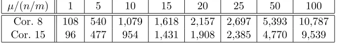
Table 2.3

This table shows the lower bounds on the number of sampled rows. The corresponding leverage score distribution is generated with Algorithm 2.6.3 and consists of as many zeros as possible. All non-zero leverage scores, expect possibly one, are equal to the coherence µ, so that ⌧ ⇡µ. The bounds are displayed for eight di↵erent values of coherence, ranging from minimal coherence µ=n/m toµ= 100n/m.

The bounds for Corollary 8 are the same as in Table 2.2, because the coherence values are the same. Since ⌧ =µ, the di↵erence between Corollaries 8 and 15 is not as drastic as in Table 2.2, yet it increases with increasing coherence. For µ = 100n/m, Corollary 15 remain informative, while Corollary 8 does not.

The goal of this section was to derive condition number bounds that are based on leverage scores rather than just coherence, when rows are sampled uniformly with replacement (Algo-rithm 2.3.2). Corollary 16 and the numerical experiments illustrate that the lower bound on the number of sampled rows implied by Corollary 15 is smaller than that from Corollary 8.

(41)

Table 2.3: Lower bounds for number of sampled rows in Corollaries 8 and 15, for di↵erent values of coherenceµ. The first value represents minimal coherenceµ=n/m. Herem= 10,000,n= 5,

=.01, ✏= 99/101, with leverage scores generated by Algorithm 2.6.3.

µ/(n/m) 1 5 10 15 20 25 50 100

Cor. 8 108 540 1,079 1,618 2,157 2,697 5,393 10,787 Cor. 15 96 477 954 1,431 1,908 2,385 4,770 9,539

measure⌧ is the same as the coherence, Corollary 15 still retains a small advantage, which can increase with increasing coherence. Hence Corollary 15 tends to remain informative for larger values of coherence, even when Corollary 8 fails.

The di↵erence in implied sampling amounts becomes more drastic in the presence widely varying non-zero leverage scores, and can be as high as ten percent. This is because the coherence-based bound in Corollary 8 cannot take advantage of the distribution of the leverage scores.

Hence, when it comes to lower bounds for the number of rows sampled uniformly with replacement, we recommend Corollary 15.

We have yet to derive leverage score based bounds for the other two sampling strategies, uni-form sampling without replacement (Algorithm 2.3.1) and Bernoulli sampling (Algorithm 2.3.3).

2.6 Algorithms for generating matrices with prescribed

coher-ence and leverage scores

In order to investigate the efficiency of the sampling methods in Section 2.3, and test the tightness of the bounds in Sections 2.4 and 2.5, we need to generate matrices with orthonormal columns that have prescribed leverage scores and coherence. The algorithms are implemented in the Matlab packagekappa SQ v3 [22].

(42)

2.6.1 Matrices with prescribed leverage scores

We present an algorithm that generates matrices with orthonormal columns that have prescribed leverage scores. In Section 2.9 we prove an existence result to show that this is always possible. Algorithm 2.6.1 is a transposed version of [9, Algorithm 3]. It repeatedly applies m⇥m Givens rotations Gij that rotate two rows iand j, and are computed from numerically stable expressions [9, section 3.1]. At most m 1 such rotations are necessary. Since each rotation a↵ects only two rows, Algorithm 2.6.1 requiresO(mn) arithmetic operations.

Algorithm 2.6.1 Generating a matrix with prescribed leverage scores [9]

Input: Integers m and nwithm n 1

Vector `with elements 0`1 · · ·`m1 andPm_j=1`j =n

Output: m_⇥nmatrixQ withQT_Q₌_I

n and leverage scoreskeTjQk22=`j, 1jm Q= In 0n⇥(m n)

T

{Initialization_}

repeat

Determine indicesi < k < j with keT_iQ_k2₂<`i,keTkQk22 =`k,keTjQk22 >`j

if `i keT_i Qk2

2 keTjQk22 `j then

Apply rotation Gij to rows iand j so that keTi GijQk22 =`i

else

Apply rotation Gij to rows iand j so that keT_jGijQk2 2 =`j

end if

Q=GijQ {Update}

until no more such indices exist

2.6.2 Leverage score distributions with prescribed coherence

We present algorithms that generate leverage score distributions for prescribed coherence. The resulting distributions then serve as inputs for Algorithm 2.6.1. These particular leverage score distribution help to distinguish the e↵ect of coherence, which is the largest leverage score, from that of the remaining leverage scores.

One large leverage score

(43)

Algorithm 2.6.2Generating a leverage score distribution with prescribed coherence: One large leverage score

Input: Integers m and nwithm n 1 Real numberµwith n/m_µ_1

Output: Vector` with elements`1=µ, 0<`j 1 andPm_j=1`j =n `1 =µ

for j= 2 :m do

`j = _mn µ₁

end for

In the special case of minimal coherence µ = n/m, Algorithm 2.6.2 generates m identical leverages equal toµ, which is the only possible leverage score distribution in this case.

Many zero leverage scores

Given a prescribed coherence, Algorithm 2.6.3 generates a distribution with as many zero lever-age scores as possible. This serves as an “adversarial” distribution for the sampling algorithms in Section 2.3.

Given a prescribed coherence µ, Algorithm 2.6.3 first determines the smallest number of rows ms that can realize this coherence, setsms 1 leverage scores equal toµ, assigns another leverage score to to take up the possibly non-zero slack, and sets the remaining leverage scores to zero.

Algorithm 2.6.3 Generating a leverage score distribution with prescribed coherence: Many zero leverage scores

Input: Integers m and nwithm n 1 Real numberµwith n/m_µ_1

Output: Vector` with elements`1=µ, 0`j 1 andPm_j=1`j =n ms=dn/µe {Number of nonzero rows}

for j= 1 :ms 1 do `j =µ

end for

`ms =n (ms 1)µ

for j=ms+ 1 :m do

`j = 0

(44)

2.6.3 Structured matrices with prescribed coherence

We present two classes of structured matrices with orthonormal columns that have prescribed coherence. Although the structure puts constraints on the matrix dimensions, the generation of these matrices is faster than running Algorithm 2.6.1. Note that the matrices produced by Algorithm 2.6.1 also have structure, but it is not easily characterized.

Stacks of diagonal matrices Given matrix dimensions m and n, where s = m/n is an integer, and prescribed coherenceµ. Them⇥nmatrixQbelow has orthonormal columns and coherence µ, and consists of sstacks ofn_⇥ndiagonal matrices,

Q= 0 B B B B @

p_{µ I} n In .. . In 1 C C C C

A where ⌘

s

1 µ

m n 1

.

Matrices with Hadamard structure Given matrix dimensions m and n, where m = 2k and n < mis also a power of two, and prescribed coherenceµ. The m_⇥nmatrix

Q=Dk In

0

!

has orthonormal columns and coherenceµ, and is defined recursively as follows. For

↵_⌘

v u u

tµ mn 11

1 _mn 1₁, ⌘

r

1 ↵2

m 1

define square matricesBj of dimension 2j and square matricesDj of dimension 2j+1 as follows,

B0 = , Bj+1 =

Bj Bj Bj Bj

!

0_j_k 1

D1 = ↵ ↵

!

, Dj+1= Dj Bj Bj Dj

!

.

(45)

2.7 Proofs for Sections 2.4 and 2.5.2

For the coherence-based bounds in Section 2.4 we first present a matrix concentration inequality (Section 2.7.1), and then the proofs of Theorem 7 (Section 2.7.2) and Corollary 8 (Section 2.7.3). For the bound based on leverage scores in Section 2.5.2, we first present a matrix concen-tration inequality (Section 2.7.4), and then the proof of Theorem 11 (Section 2.7.5).

2.7.1 Matrix Cherno↵ Concentration inequality

The matrix concentration inequality below is the basis for Theorem 7 and Corollary 8.

Denote the eigenvalues of a Hermitian matrix Z by j(Z), and the smallest and largest eigenvalues by min(Z)⌘minj j(Z) and max(Z)⌘maxj j(Z), respectively.

Theorem 17 (Corollary 5.2 in [37]) LetXj be a finite number of independent randomn⇥n Hermitian positive semidefinite matrices with maxjkXjk2 ⌧. Define

!min ⌘ min

0

@X

j

E[Xj]

1

A !max ⌘ max

0

@X

j

E[Xj]

1