Life Cycle Inventory Incorporating Fuel Cycle and Real-World In-Use Measurement Data for Construction Equipment and Vehicles.

(1)

ABSTRACT

PANG, SHIH-HAO. Life Cycle Inventory Incorporating Fuel Cycle and Real-World In-Use Measurement Data for Construction Equipment and Vehicles. (Under the direction of Dr. H. Christopher Frey.)

Biodiesel is an alternative fuel that can be made from vegetable oils or animal fat. This

study focuses on whether substitution of soy-based biodiesel fuels for petroleum diesel

would produce an overall reduction in emissions of selected pollutants. A life cycle

inventory model was developed to estimate energy consumption and emissions of

selected pollutants and greenhouse gases. Real-world measurements using portable

emission measurement system (PEMS) were made for 15 construction vehicles, including

five backhoes, four front-end loaders, and six motor graders on both petroleum diesel and

soy-based B20 biodiesel. These data are used as the basis for vehicle tailpipe emission

factors of CO2, CO, HC, NOx, and PM. The results imply that biodiesel is a promising

alternative fuel for diesel, but that there are some environmental trade-offs. Analysis of

empirical data reveals that intra-vehicle variability of energy use and emissions is

strongly influenced by vehicle activity that leads to variations in engine load, as

represented by manifold absolute pressure (MAP). Vehicle-specific models for fuel use

(2)

The time-based regression model has the highest explanatory ability among six models

and is recommended in order to predict fuel use and emission rate for diesel-fueled

nonroad construction equipment. Representative duty cycles for each type of vehicles

were characterized by a frequency distribution of normalized manifold absolute pressure

(MAP). In order to assess the variations of fuel use and emissions among different duty

cycles, for a given engine, the inter-cycle variability is assessed. In order to assess the

variations of fuel use and emissions among engines, for a given duty cycle, the

engine variability is assessed. The results indicated time-based cycle and

inter-engine variations of fuel use and emissions are significant. Fuel-based emission factors

have less variability among cycles and engines than time-based emission factors.

Fuel-based emission factors are more robust with respect to inter-engine and inter-cycle

variations and are recommended in order to develop an emissions inventory for nonroad

construction vehicles. Real-world in-use measurements should be a basis for developing

(3)

Life Cycle Inventory Incorporating Fuel Cycle and Real-World In-Use Measurement

Data for Construction Equipment and Vehicles

by

Shih-Hao Pang

A dissertation submitted to the Graduate Faculty of

North Carolina State University

In partial fulfillment of the

Requirements for the degree of

Doctor of Philosophy

Civil Engineering

Raleigh, NC

2007

APPROVED BY:

Dr. E. Downey Brill Jr. Dr. William Rasdorf

(4)

BIOGRAPHY

Shih-Hao Pang was born on the 11th of December, 1976 in Taipei, Taiwan. He got his

Bachelor’s Degree in Atmospheric Science from National Taiwan University, Taiwan, in

1999. After his graduation, he started his graduate studies in the Graduate Institute of

Environmental Engineering in National Taiwan University. He worked on

photochemical trajectory air quality modeling and got his Master’s Degree in 2001. He

came to North Carolina State University for his Doctoral Degree in Environmental

Engineering in 2004. He was a research assistant in Dr. H. Christopher Frey’s research

group, and his research was focused on life cycle inventory for petroleum diesel and

biodiesel fuels, assessment of on-board emissions measurements of nonroad construction

equipment and vehicles, and emissions modeling. This dissertation completes the

requirements for this degree.

(5)

ACKNOWLEDGEMENTS

This material is based upon work supported by the National Science Foundation under

Grant No. 0327731. Any opinions, findings, and conclusions or recommendations

expressed in this material are those of the author(s) and do not necessarily reflect the

views of the National Science Foundation.

I would like to express my appreciation to Dr. H. Christopher Frey for his continues

guidance and valuable technical suggestions throughout the course of this work. Without

Dr. Frey’s suggestion and guidance, this work would not have been in its current form. I

would like to thank Dr. W. Rasdorf and other committee members, Dr. E.D Brill and Dr.

D. van der Vaart for their suggestions and assistances. I would like to thank Dr. Jon Van

Gerpen, Dr. Carl J Bern, Dr. Dev Shrestha, Dr. Larry Johnson, Dr. Alex Hobbs, Mr. Jim

Wilder, Mr. Andy Aden, Mr. Vince Vavpot, and Mr. Bev Thessen provided useful

information and suggestions for the life cycle study. I would like also to thank my

co-workers, Kaishan, Saeed, Kangwook, Phil, Haibo, Po-Yao, and Hyunk-Wook for helping

me with any questions that I had and giving me company in the times of hard work.

Last, but certainly not least, I would like to thank my parents, my wife, my son, my

sisters, and my mother-in-law for their sincere love, enormous support and enthusiasm

for my education. Without their endless encouragement and support, this work could not

have been possible.

(6)

TABLE OF CONTENTS

LIST OF TABLES ... vi

LIST OF FIGURES ... ix

PART I INTRODUCTION ... 1

1.1 Instrumentation ... 6

1.2 Research Objectives... 7

1.3 Organization... 8

1.4 References... 11

PART II FIELD DATA COLLECTION PROCEDURES ON NONROAD CONSTRUCTION EQUIPMENT... 13

2.1 Pre-Installation... 13

2.2 Installation... 34

2.3 Data Collection ... 41

2.4 Decommissioning ... 44

2.5 Cleanup after Data Collection... 50

2.6 Problems and Solutions for Field Measurement... 58

PART III DATA SCREENING AND QUALITY ASSURANCE... 76

3.1 Montana System, Preliminary Data Validity Check ... 77

3.2 Data Quality Checks Associated With Intake Air Temperature ... 82

3.3 Identification and Evaluation of the Effects of Air Leakage on Data Quality... 86

PART IV VEHICLE-SPECIFIC EMISSIONS MODELING FOR NON-ROAD CONSTRUCTION EQUIPMENT BASED UPON REAL-WORLD MEASUREMENTS... 107

Abstract ... 107

4.1 Introduction... 109

4.2 Methodology... 112

4.3 Results... 126

4.4 Discussion... 145

PART V CHARACTERIZATION OF INTER-CYCLE AND INTER-ENGINE VARIABILITY FROM DIESEL POWERED NON-ROAD CONSTRUCTION VEHICLES ... 149

Abstract ... 149

5.1 Introduction... 150

5.3 Results... 164

(7)

PART VI REVIEW OF PREVIOUS LIFE CYCLE STUDIES... 191

6.1 The Greenhouse Gases, Regulated Emissions, and Energy consumption in Transportation (GREET) Model ... 191

6.2 Lifecycle Emissions Model (LEM) ... 192

6.3 GM Well-to-Wheel North American Study ... 193

6.4 Economic Input-Output Life-Cycle Analysis Model... 194

6.5 National Renewable Energy Laboratory Study ... 195

6.6 Other Life Cycle Studies... 196

PART VII DEVELOPMENT OF LIFE CYCLE INVENTORY FOR PETROLEUM DIESEL AND BIODIESEL FUELS... 210

7.1 Definition of LCI System Boundaries ... 211

7.2 Estimations of Energy Use and Emissions for Well-to-Pump Stages... 216

7.3 Vehicle Tailpipe Emissions ... 226

7.4 Model Inputs and Parameters... 229

7.5 Probability Distribution of Inputs for Uncertainty Analysis... 234

PART VIII LIFE CYCLE INVENTORY ENERGY CONSUMPTION AND EMISSIONS FOR BIODIESEL VERSUS PETROLEUM DIESEL FUELED CONSTRUCTION VEHICLES ... 271

Abstract 271 8.1 Introduction... 272

8.3 Results... 288

PART IX CONCLUSIONS AND RECOMMENDATIONS ... 303

9.1 Conclusions... 303

9.2 Recommendations for Future Work... 309

APPENDIX A MEASURED TIME-BASED MODAL FUEL USE AND EMISSION RATES AND FUEL-BASED EMISSION RATES FOR ENGINE AND TASK ORIENTED MODES FOR ALL TESTED VEHICLES ... 311

APPENDIX B. COEFFICIENTS OF PHYSICALLY REGRESSION MODELS FOR EACH TESTED VEHICLE ... 654

(8)

LIST OF TABLES

PART II FIELD DATA COLLECTION PROCEDURES ON NONROAD CONSTRUCTION EQUIPMENT

Table 2.1 Pre-installation Checklist Form ... 16

Table 2.2 Typical Time Period and Range for Pre-installation ... 19

Table 2.3 Installation Checklist Form... 36

Table 2.4 Typical Time Period and Range for Installation Based on Equipment Type... 37

Table 2.5 Data Collection Checklist Form... 43

Table 2.6 Decommissioning Checklist Form... 45

Table 2.7 Cleanup Checklist Form ... 51

Table 2.8 Problems and Solutions during Data Collection... 73

PART III DATA SCREENING AND QUALITY ASSURANCE Table 3.1 Indicators Flagged by the Montana System... 79

Table 3.2 Examples of Data Flagged as Valid and Invalid... 81

Table 3.3 Equivalent Molecular Formulas for Diesel, Biodiesel B20, and Biodiesel B100... 92

Table 3.4 An Example of One Second of Emission Data from a Generator Tested on November 11, 2005... 93

Table 3.5 Example Case Study of the Predicted Effect of Air Leakage on Observed Concentrations of Pollutants from a Generator Tested on November 11, 2005... 93

Table 3.6 Mass Emission Rate of Each Pollutant at Different Ratio of Oxygen to Fuel from a Generator Tested on November 11, 2005... 95

Table 3.7 Case Study of One Second of Emission Data below the Precision of the Montana System ... 98

Table 3.8 Case Study of the Observed and Predicted Emission Data on a Dry Basis from an Off-Highway Truck Tested on February 09, 2006 ... 99

Table 3.9 Input Assumptions for Uncertainty Analysis...100

Table 3.10 95% Probability Range of Mass Emission Rates of One Second of Data below the Precision of the Montana System ...101

Table 3.11 95% Probability Range of Mass Emission Rates of One Second of Data from an Off-Highway Truck Tested on February 09, 2006 ...101

Table 3.12 Application of Criteria for Air-to-Fuel Ratio to Six Pieces of Construction Equipment ...105

(9)

PART IV VEHICLE-SPECIFIC EMISSIONS MODELING FOR NON-ROAD CONSTRUCTION EQUIPMENT BASED UPON REAL-WORLD MEASUREMENTS

Table 4.1 Characteristics of Tested Vehicles...115 Table 4.2 Rank Correlation of Fuel Use and Emissions With Respect to

Engine Data Based on Front-End Loader 1 ...128 Table 4.3 Coefficient of Determination of Time-Based Engine-Based Modal

Models for Fuel Use and Emissions ...133 Table 4.4 Coefficient of Determination of Fuel-Based Engine-Based Modal

Models for Fuel Use and Emissions ...134 Table 4.5 Coefficient of Determination of Time-Based Task-Based Modal

Models for Fuel Use and Emissions ...135 Table 4.6 Coefficient of Determination of Fuel-Based Task-Based Modal

Models for Fuel Use and Emissions ...136 Table 4.7 Coefficient of Determination of Time-Based Regression Models

for Fuel Use and Emission Rates ...140 Table 4.8 Coefficient of Determination of Fuel-Based Regression Models for

Fuel Use and Emissions ...141 Table 4.9 Benchmarks of Weighted Average Emission Rates Based on

NONROAD Model ...143

PART V CHARACTERIZATION OF CYCLE AND INTER-ENGINE VARIABILITY FROM DIESEL POWERED NON-ROAD CONSTRUCTION VEHICLES

Table 5.1 Inter-Engine and Inter-Cycle Variations of Time-Based Fuel Use

Rates (g/sec)...170 Table 5.2 Inter-Engine and Inter-Cycle Variations of Time-Based NOx

Emission Rates (mg/sec)...172 Table 5.3 Inter-Engine and Inter-Cycle Variations of Fuel-Based NOx

Emission Rates (g/gal) ...175 Table 5.4 Ratio of High versus Low Value for Cycle Average Time-Based

Fuel Use and Emission Rates Based on Comparisons of 16 Duty

Cycles for Engines of Each of 30 Tested Engines...177 Table 5.5 Ratio of High versus Low Value for Cycle Average Fuel-Based

Emission Rates Based on Comparisons of 16 Duty Cycles for

Engines of Each of 30 Tested Engines ...179 Table 5.6 Ratio of High versus Low Value for Cycle Average Time-Based

Fuel Use and Emission Rates Based on Comparisons of 30 Engines

for Each of 16 Duty Cycle ...185 Table 5.7 Ratio of High versus Low Value for Cycle Average Fuel-Based

Emission Rates Based on Comparisons of 30 Engines for Each of

16 Duty Cycle ...186

(10)

PART VI REVIEW OF PREVIOUS LIFE CYCLE STUDIES

Table 6.1 A Comparison of Previous Life Cycle Models...202

PART VII DEVELOPMENT OF LIFE CYCLE INVENTORY FOR PETROLEUM DIESEL AND BIODIESEL FUELS Table 7.1 Estimate of 2002 U.S. National Average Emission Factors of Utility Boiler ...222

Table 7.2 Estimate of 2002 U.S. National Average Emission Factors of Industrial Boiler ...223

Table 7.3 Comparison of 2002 U.S. National Average Emission Factors with GREET 1.6 Model, Utility Boiler...224

Table 7.4 Comparison of 2002 U.S. National Average Emission Factors with GREET 1.6 Model, Industrial Boiler...225

Table 7.5 Characteristics of Tested Vehicles...227

Table 7.6 Petroleum Diesel LCI: Feedstock and Product...230

Table 7.7 Biodiesel B100 LCI: Feedstock and Product...230

Table 7.8 Energy Efficiencies for Petroleum Diesel Fuel Cycle ...232

Table 7.9 Transportation Distance for Petroleum Diesel LCI ...232

Table 7.10 Transportation Distance for Biodiesel B100 LCI ...233

Table 7.11 Energy Use for Petroleum Diesel and Biodiesel Fuel Cycle ...233

Table 7.12 Probability Distributions of Uncertain Inputs for Petroleum Diesel Life Cycle...235

Table 7.13 Probability Distribution of Uncertain Inputs for Biodiesel Life Cycle ...251

PART VIII LIFE CYCLE INVENTORY ENERGY CONSUMPTION AND EMISSIONS FOR BIODIESEL VERSUS PETROLEUM DIESEL FUELED CONSTRUCTION VEHICLES Table 8.1 Characteristics of Tested Vehicles...282

Table 8.2 Study Design of Life Cycle Inventory ...285

Table 8.3 Example of Key Input Assumptions and Best Estimates of Petroleum Diesel and Biodiesel LCI for Front-End Loader 1 Based on NCSU In-Use Measurement Data...287

Table 8.4 Average Percentage Difference (%) of B20 versus Petroleum Diesel in LCI Emissions per Gallon of Diesel Equivalent ...291

Table 8.5 Proportion of Vehicle Tailpipe Emissions to Total LCI Emissions Based on Vehicle Types and Engine Tier (NCSU In-Use Measurement data)...292

(11)

LIST OF FIGURES

PART II FIELD DATA COLLECTION PROCEDURES ON NONROAD CONSTRUCTION EQUIPMENT

Figure 2.1 Timeline for Pre-installation Procedures Performed by Two People ... 18

Figure 2.2 Safety Cage for Montana Installation ... 20

Figure 2.3 Safety Cage on a Backhoe ... 21

Figure 2.4 Safety Cage on a Motor Grader ... 21

Figure 2.5 Attachment of Exhaust Gas Sampling Probes to the Tailpipe... 22

Figure 2.6 Attachment of the Sampling Hose to the Main Unit... 23

Figure 2.7 Illustration of a Typical Gap between Muffler and Tailpipe ... 24

Figure 2.8 Sealing a Gap Using Aluminum Foil and Hose Clamps... 24

Figure 2.9 Illustration of MAP Port ... 26

Figure 2.10 MAP Port on the Engine and a Barb Fitting Attached to the Port... 26

Figure 2.11 MAP Sensor after Installation... 27

Figure 2.12 Magnetized Engine Speed Sensor Attached on the Metal ... 28

Figure 2.13 Engine Speed Sensor and Optical Tape ... 29

Figure 2.14 Installation of Intake Air Temperature Sensor... 30

Figure 2.15 Sensor Unit on a Bulldozer ... 31

Figure 2.16 External Battery Setup for Montana System Power Source ... 32

Figure 2.17 Timeline for Installation Procedures Performed by Two Persons ... 37

Figure 2.18 Trimble GPS Receiver ... 39

Figure 2.19 Synchronization of the Camcorder and the Laptop Computer ... 41

Figure 2.20 Timeline for Data Collection Procedures ... 44

Figure 2.21 Timeline for Decommissioning Performed by One Person... 47

Figure 2.22 Timeline for Decommissioning Performed by Two Persons... 48

Figure 2.23 Parts of the Montana Addressed in the Cleaning Procedure... 53

Figure 2.24 Illustration of a Stabilized Pressure Sensor ... 63

Figure 2.25 Illustration of an Engine Speed Sensor and Optical Tape ... 65

Figure 2.26 Gap between Muffler and Tailpipe ... 70

Figure 2.27 Sealing the Gap between Muffler and Tailpipe ... 70

(12)

PART III DATA SCREENING AND QUALITY ASSURANCE

Figure 3.1 Cumulative Frequency of the Difference of Intake Air Temperature between Consecutive Seconds Based on a Backhoe Tested on

December 30, 2005 ... 83 Figure 3.2 Cumulative Frequency of the Difference of Intake Air Temperature

between Consecutive Seconds Based on a Skid Steer Loader

Tested on January 20, 2006 ... 85 Figure 3.3 Cumulative Frequency of Air-to-Fuel Ratio for Different

Construction Equipment, with Type of Equipment and Data of

Field Measurement Indicated... 97 Figure 3.4 Flow Diagram of the Evaluation Procedures for Air-to-Fuel Ratio ...104

PART IV VEHICLE-SPECIFIC EMISSIONS MODELING FOR NON-ROAD CONSTRUCTION EQUIPMENT BASED UPON REAL-WORLD MEASUREMENTS

Figure 4.1 Example of a Time Series Plot of Manifold Absolute Pressure,

Fuel Use, and NO Emission Rate for a Front-End Loader ...129 Figure 4.2 Observed Fuel Use and Emissions versus Predicted Fuel Use and

Emissions Based on Time-Based Engine-Based Modal Models for

Excavator 1 ...131 Figure 4.3 Observed Fuel Use and Emissions versus Predicted Fuel Use and

Emissions Based on Time-Based Task-Oriented Modal Models for

Excavator 1 ...132

PART V CHARACTERIZATION OF CYCLE AND INTER-ENGINE VARIABILITY FROM DIESEL POWERED NON-ROAD CONSTRUCTION VEHICLES

Figure 5.1 Cumulative Frequency Distribution of MAP for All Duty Cycles ...167 Figure 5.2 Scatter Plot of Time-Based and Fuel-Based NO Emission Rate

versus Engine Displacement Based on Duty Cycle 11...187

(13)

PART VII DEVELOPMENT OF LIFE CYCLE INVENTORY FOR PETROLEUM DIESEL AND BIODIESEL FUELS

Figure 7.1 Diagram of Life Cycle Inventory for Petroleum Diesel ...212

Figure 7.2 Detailed Diagram of Stage 4 of Petroleum Diesel Life Cycle...213

Figure 7.3 Detailed Diagram of Stage 5 of Petroleum Diesel Life Cycle...214

Figure 7.4 Diagram of Life Cycle Inventory for Biodiesel...215

Figure 7.5. Example of Allocation of Process Fuel among Life Cycle Inventory...218

Figure 7.6 Process Energy for Petroleum Diesel and B100 LCI...231

PART VIII LIFE CYCLE INVENTORY ENERGY CONSUMPTION AND EMISSIONS FOR BIODIESEL VERSUS PETROLEUM DIESEL FUELED CONSTRUCTION VEHICLES Figure 8.1 System Boundaries for Petroleum Diesel and Biodiesel Life Cycle Inventory...278

Figure 8.2 Example of Life Cycle Inventory (LCI) Results for Scenario (1), (2), and (5) ...290

Figure 8.3 Fossil Energy Consumption for Petroleum Diesel, B20, and B100 LCI per Gallon of Petroleum Diesel Equivalent...293

Figure 8.4 Soybean Yield, Biodiesel Plants and Air Quality in the U.S...296

Figure 8.5 Comparison of Local Urban and Total Emissions Based on the Average of 15 NCSU Tested Vehicles ...297

(14)

1

PART I INTRODUCTION

In 2002, annual emissions of nonroad diesel construction vehicles for carbon monoxide

(CO), volatile organic compounds (VOC), nitrogen oxides (NOx), and particulate matter

(PM10) were 414, 85, 764 and 71 thousand short tons, respectively. These emissions are

significant, yet they only include direct emissions from the vehicle and they do not

include life cycle emissions from the fuel cycle. An improved quantitative understanding

of life cycle emissions is needed in order to assess the role of these vehicles in air quality

problems and to develop management strategies.

Nonroad diesel powered equipment is coming under increased scrutiny because it is a

significant source of nonroad mobile source air pollutant emissions. Emissions from

nonroad construction equipment are typically quantified based on steady-state engine

dynamometer tests. However, such tests do not represent actual duty cycles. Emission

inventory developed based on these steady-state engine dynamometer tests can not

represent real-world emissions. Therefore, there is a need to quantify energy use and

emissions from construction equipment based on in-use measurement methods.

Compared with other types of vehicles, there has been relatively little real world

measurement of in-use emissions of nonroad diesel powered vehicles. There is a need to

develop a set of standard procedures for field data collection and analysis for this

(15)

2

In the United States, more than half of the biodiesel is made from soybean oil. The

production of biodiesel accounted for 1.42% of total U.S. soybean oil consumption in

2004. Biodiesel can be used in a diesel engine without major modifications and has

lower emissions of hydrocarbon (HC), carbon monoxide (CO), and particulate matters

(PM) based on dynamometer testing of engines (EPA 2002). Based on engine

dynamometer data from EPA and chassis dynamometer data from National Renewable

Energy Laboratory (NREL), the percentage changes when comparing B20 biodiesel

versus petroleum diesel of NOx, PM, CO, and HC are +2%, -10%, -11%, and -21%,

respectively, for the EPA data and +0.6%, -16%, -17%, and -12%, respectively, for the

NREL data (EPA 2002, McCormick et al. 2006). The recent NREL study agrees on the Frey and Kim (2006) and other studies that show a decrease in NOx for B20 if the blend

stock meets the ASTM standard.

Biodiesel has several advantages, e.g., it is biodegradable, and non-toxic, and it has the

potential of reducing U.S. dependence on foreign crude oil. Because of the Energy

Policy Act of 2005, many government agencies are already using biodiesel in their

(16)

3

Nonroad construction equipment is a significant source of nonroad mobile source air

pollutant emissions. Three common types of construction vehicles are backhoes,

front-end loaders, and motor graders. These vehicles contribute to 26.5% of NOx, 29.1% of

CO, 27.6% of HC and 28.3% of PM10 among all construction vehicles. In-use

measurements on construction vehicles were described by Frey et al. (2007). Data collection procedures include: (1) pre-installation; (2) installation; (3) field data

collection; and (4) decommissioning. Field data were reviewed by standard quality

assurance procedures to determine whether any errors exist in the data, and corrected

such errors if possible. Emission factors of HC, CO, NOx, and PM were developed based

on typical duty cycles performed by each vehicle.

Life cycle inventories are used for a more complete assessment of comparisons between

fuels, taking into account energy consumption, and emissions for fuel production and fuel

use. Life cycle inventory approaches, include process flow diagrams, matrix

representation of product system, and input-output-based LCI. Process flow diagrams are

the most common method for representing the energy use and emissions of processes in a

product system (MacLean et al. 2003, Sheehan et al. 1998, Suh et al. 2005). An example is the Greenhouse Gases, Regulated Emissions, and Energy use in Transportation

(GREET) model. GREET has been used to estimate fuel cycle upstream energy use and

air emissions in life cycle inventories of bio-based products and lubricants (Landis et al.

(17)

4

Sheehan et al. conducted a study of soy-based biodiesel and petroleum diesel life cycles in 1998. The study quantified environmental flows associated with soy-based biodiesel

and petroleum diesel. The result indicated soy-based B20 biodiesel has lower life cycle

emissions of carbon monoxide and particulate matters, but higher LCI emissions of

nitrogen oxides (NOx) and hydrocarbons (HC). However, this study was based on old

soyoil plant, which is not subject to the new emission standards in 2004, and EPA engine

dynamometer data. The EPA engine dynamometer data showed a 2% increase of vehicle

tailpipe NOx emissions when comparing B20 versus petroleum diesel. In recent study,

the use of B20 biodiesel does not have significant change or perhaps a decrease in NOx

(McCormick et al. 2006).

Soy-based B100 biodiesel production includes three major processes: soybean farming,

soybean oil extraction, and biodiesel production. In the United States, most soybean oil

production plants use a solvent extraction process to remove the oil from the soybeans

(Erickson 1995). Soybean oil extraction was found to be the most significant source of

HC emissions in the biodiesel life cycle (Sheehan et al. 1998). In November 2004, EPA promulgated national emission standards for the solvent extraction process (EPA 2004).

The standards require reduction of emissions of air toxics and volatile organic

(18)

5

An improved quantification of the life cycle inventory (LCI) is developed here in order to

evaluate the benefits of biodiesel and to assess the tailpipe emissions of selected types of

construction vehicles. The key improvements include the use of PEMS data for

real-world fuel use and emissions and comparisons based on 15 construction vehicles which

(19)

6

1.1 Instrumentation

A portable emission measurement system (PEMS) was used for real world in-use data

collection developed by Clean Air Technologies International, Inc. The PEMS is

comprised of two identical gas analyzers, a particulate matter (PM) measurement system,

an engine diagnostic scanner or sensor array, a global position system (GPS), and an

on-board computer. This system is designed to measure mass emission rates under actual

operating conditions of a vehicle using engine operating data and concentration of

pollutants in the exhaust.

The engine data is obtained from either the engine scanner, which is used when an engine

has an electronic diagnostic link, or a sensor array, which can be used as long as the

engine has a port to which the manifold absolute pressure (MAP) sensor can be attached.

The sensor array is composed of a MAP sensor, an engine speed sensor, and an intake air

(20)

7

The concentrations for nitric oxide (NO), hydrocarbons (HC), carbon monoxide (CO),

carbon dioxide (CO2), and oxygen (O2) in the vehicle exhaust measured by the gas

analyzer are expressed in parts per million or volume percentage. The PM measurement

device includes a laser light scattering detector that is basically an opacity type of

measurement, and a sample conditioning system. The results of the PM measurement

have been correlated to a mass per volume basis by the instrument vendor. A global

positioning system (GPS) is used to measure the vehicle position. The on-board

computer synchronizes the incoming emissions, engine, and GPS data. Intake airflow,

exhaust flow, and mass emissions are estimated using a method reported by

Vojtisek-Lom and Cobb (1997).

1.2 Research Objectives

The key research objectives are:

– Develop a life cycle inventory (LCI) model for energy consumption and

emission of criteria pollutants and greenhouse gases. This LCI will support the

future development of rigorous life cycle assessment and impact analyses for

the purposes of air quality management

– Recommend a set of standard procedures for field data collection and analysis

(21)

8

– Characterize the second-by-second in-use emissions and energy use of

nonroad construction vehicles and equipment, including emissions of nitric

oxide (NO), carbon monoxide (CO), hydrocarbons (HC), carbon dioxide

(CO2), and particulate matters (PM)

– Develop a predictive micro-scale emission model to estimate energy use and

emissions for a wide variety of activity patterns

1.3 Organization

Part I describes general information regarding nonroad construction vehicle emissions,

production of biodiesel, life cycle inventory, and the needs for development of life cycle

inventory for petroleum diesel and biodiesel fuels, the research objectives.

Part II explains the general procedures for portable on-board emissions data collection

when collecting data on nonroad construction vehicle, including front-end loaders,

backhoes, and motor graders. These procedures are good for all nonroad construction

vehicles and equipment.

Part III describes data screening and quality assurance procedures for reviewing data

collected in the field, determining whether any errors or problems exist in the data,

correcting such errors or problems where possible, and removing invalid data if errors or

(22)

9

Part IV is a draft paper and applies recently collected in-use data to gain insight into

real-world variability in fuel use and emissions for individual vehicles. Analysis of empirical

data reveals that intra-vehicle variability of energy use and emissions is strongly

influenced by vehicle activity that leads to variations in engine load, as represented by

manifold absolute pressure (MAP). Vehicle-specific models for fuel use and tailpipe

emissions were developed for each of the 32 construction vehicles.

Part V is a draft paper to characterize real-world variability in fuel use and emissions

when comparing vehicles and duty cycles. Representative duty cycles for each type of

vehicles were characterized by a frequency distribution of normalized manifold absolute

pressure (MAP). Vehicle-specific models for fuel use and tailpipe emissions were

developed for each of the construction vehicle based on physically-based regression

model. In order to assess the variations of fuel use and emissions among different duty

cycles, for a given engine, the inter-cycle variability is assessed. In order to assess the

variations of fuel use and emissions among engines, for a given duty cycle, the

inter-engine variability is assessed.

Part VI gives the reviews of previous life cycle studies and a comparison of each life

(23)

10

Part VII gives the methodology of life cycle inventory development, including the fuel

life cycle and characterizing in-use emissions and energy use from nonroad construction

vehicles and equipment.

Part VIII is a draft paper and focuses on whether substitution of soy-based biodiesel fuels

for petroleum diesel would produce an overall reduction in emissions of selected

pollutants. A life cycle inventory model was developed to estimate energy consumption

and emissions of selected pollutants and greenhouse gases.

The main conclusions of this study and the recommendations for future are given in Part

(24)

11

1.4 References

Duffield, J., Shapouri, H., Graboski, M., McCormick, R., Wilson R. (1998), “U.S. Biodiesel Development: New Markets for Conventional and Genetically Modified Agricultural Fats and Oils,” Economic Research Service/U. S. Department of Agriculture,

Washington D.C.

EPA (2002), “A comprehensive analysis of biodiesel impacts on exhaust emissions,” EPA 420-P-02-001, U.S. Environmental Protection Agency, Washington D.C.

McCormick, R. L., A. Williams, J. Ireland, M. Brimhall, R.R. Hayes (2006), “Effects of Biodiesel Blends on Vehicle Emissions,” NREL/MP-540-40554, Prepared by National Renewable Energy Laboratory for U.S. Department of Energy, October.

Frey, H.C., and K. Kim (2006), “Comparison of Real-World Fuel Use and Emissions for Dump Trucks Fueled with B20 Biodiesel Versus Petroleum Diesel,” Transportation Research Record, 1987:110-117.

Energy Policy Act of 2005 (2005), PUBLIC LAW 109–58, August 8.

Frey, H.C., W.R. Rasdorf, K. Kim, S. Pang, P. Lewis, S. Abolhasani (2007), “Real-World Duty Cycles and Utilization for Construction Equipment in North Carolina,” Draft Final Report, Prepared by North Carolina State University for North Carolina Department of Transportation, Raleigh, NC, August.

MacLean, H. L.; Lave, L. B. (2003), “Evaluating automobile fuel/propulsion system technologies,” Progress in Energy and Combustion Science, 29(1): 1–69.

Sheehan, J., Camobreco, V., Duffield, J., Graboski, M., Shapouri, H. (1998), “Life Cycle Inventory of Biodiesel and Petroleum Diesel for Use in an Urban Bus,” NREL/SR-580-24089, Prepared by National Renewable Energy Laboratory for U.S. Department of Agriculture and U.S. Department of Energy, Golden, Colorado.

Suh S., Huppes, G. (2005), “Methods for Life Cycle Inventory of a Product,” Journal of Cleaner Production, 13(7): 687-697.

(25)

12

Miller S. A., A. E. Landis, T. L. Theis, R. A. Reich (2007), “A Comparative Life Cycle Assessment of Petroleum and Soybean-Based Lubricants,” Environ. Sci. Technol., 41(11): 4143-4149.

Erickson, D. R., Ed. (1995), Practical Handbook of Soybean Processing and Utilization, AOCS Press: Champaign, Illinois and the United Soybean Board: St. Louis, Missouri, Chapter 5-6.

EPA (2004), National Emission Standards for Hazardous Air Pollutants: Solvent Extraction for Vegetable Oil Production – Federal Register. 40 CFR Part 63, Vol. 69, No. 169, U.S. Environmental Protection Agency, Washington D.C.

(26)

13

PART II FIELD DATA COLLECTION PROCEDURES ON NONROAD CONSTRUCTION EQUIPMENT

The objective of this section is to explain the general procedures for portable on-board

emissions data collection when collecting data on nonroad construction vehicle, such as

front-end loaders, backhoes, and motor graders. These procedures are for nonroad

construction vehicles and equipment. These procedures include pre-installation,

installation, field data collection, decommissioning, and cleanup. For each of these major

steps of data collection, a checklist and explanation of procedures is given.

2.1 Pre-Installation

Construction workers usually start working in the early morning. In order to have

sufficient time to install the Montana system and not to interfere with their work, the data

collection crew installs some of the major components the day before a test. This is

(27)

14

Pre-installation involves installing the sensors, sampling hoses, the safety cage, the cables,

and the connections, except for the final installation of the main unit. The main unit is

installed in the morning of data collection. It typically takes two people two to three

hours to finish a pre-installation procedure. The pre-installation differs from installation

because pre-installation is done the day before a test, typically in the afternoon.

Pre-installation includes the installation of the major test system components on the test

vehicle, except for the instrument itself. The following sections explain these major

components and installation procedures. Table 2.1 shows the checklist for

pre-installation. Two people are needed to finish pre-pre-installation. Even with two people

working together pre-installation takes a minimum of two hours and forty minutes.

Figure 2.1 shows the timeline for pre-installation when performed by two people. Due to

different engine models and ambient conditions, the time period for pre-installation may

vary from two hours and forty minutes to three hours and forty minutes. Each of the

items of equipment has a different engine model and engine compartment room shape. In

some cases, pre-installation of engine sensors is very difficult due to the small engine

compartment room. If the data collection crew cannot locate the port for the manifold

(28)

15

When a new construction vehicle is to be tested (of a type not previously tested by the

data collection crew) the data collection crew needs additional time to find the

appropriate place to install engine sensors. When the same model of construction

equipment is to be tested again, two hours and forty minutes is usually enough for

pre-installation. Table 2.2 presents typical pre-installation time period and pre-installation

time range for a backhoe, motor grader, and front-end loader.

The height of equipment presents also another difficulty for completing test equipment

pre-installation. Working at 9 to 11 feet high from the ground and on the limited space of

the roof of the construction equipment is not easy. These roofs were not initially

designed for someone to be working on there. This area is very slippery and not safe.

Extra care must be taken to ensure safety. For this reason, pre-installation may also need

more time to be completed.

When pre-installation is completed, the main unit of the Montana system will be brought

to the laboratory and calibrated. There is a gap in time between pre-installation

completion and calibration, because of the traveling time from the construction site to the

(29)

16

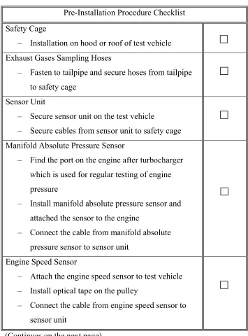
Table 2.1 Pre-installation Checklist Form

Pre-Installation Procedure Checklist Safety Cage

– Installation on hood or roof of test vehicle Exhaust Gases Sampling Hoses

– Fasten to tailpipe and secure hoses from tailpipe to safety cage

Sensor Unit

– Secure sensor unit on the test vehicle

– Secure cables from sensor unit to safety cage Manifold Absolute Pressure Sensor

– Find the port on the engine after turbocharger which is used for regular testing of engine pressure

– Install manifold absolute pressure sensor and attached the sensor to the engine

– Connect the cable from manifold absolute pressure sensor to sensor unit

Engine Speed Sensor

– Attach the engine speed sensor to test vehicle – Install optical tape on the pulley

– Connect the cable from engine speed sensor to sensor unit

(30)

17 Table 2.1 Continued.

Intake Air Temperature Sensor

– Install intake air temperature sensor

– Fix the intake air temperature sensor near the intake air flow using duct tape or plastic wire – Connect the cable from intake air temperature

sensor to sensor unit External Power Source

– Install external power source – Secure power cable to safety cage Measurement Instrument Pre-test

– Install main unit of Montana system – Connect sensor unit to main unit

– Read engine data to decide if it is necessary to re-install engine sensors

Re-installation (if engine sensor is not installed properly) – Re-install sensors

Re-test (after re-install sensors)

– Read engine data to decide if it is necessary to re-install engine sensors again

Wrap-up

– Pick up tools and put into the toolbox Calibration of Montana System

– Warm up the main unit for forty-five minutes – Perform calibration procedures according to

(31)

18

Figure 2.1 Timeline for Pre-installation Procedures Performed by Two People 30 Safety Cage S 00:0 00:3 Sampling Hose Setup 20 00:5 MAP Sensor Setup 30 RPM Sensor Setup 30 00:30 01:0 30 Air Temperature Sensor Setup 01:30 External Power Setup 20 01:30 Sensor Unit Setup 20 01:1 Pre-test

10 30

Re-installation

(if necessary) Test

10

Wrap Up

10

01:40 _{02:10 02:20}

Durations of individual

02:10 Cumulative time (in hours:minutes) from the start of the activity 30 min

02:40 ……

…… ₁₀ Cali-bration

01:30

Pre-test

10 30

Re-installation

(if necessary) Test

10

Wrap Up

10

01:40 02:10 02:20

(32)

19

Table 2.2 Typical Time Period and Range for Pre-installation

Pre-Installation Time Period Equipment Type

Typical Range

Backhoe 2 hr 40 min

2 hr 40 min to 3 hr 40 min

Motor Grader 2 hr 40 min

Front-End Loader 2 hr 40 min

2.1.1 Safety Cage

To protect the Montana system from damage, and to help control transmission of

vibration from the vehicle to the Montana system, a hard metal safety cage has been

developed. The cage is large enough to enclose the main unit of the Montana system.

The cage is intended to protect the main unit from being impacted by tree branches or

other potential obstacles that might be encountered at a construction site.

Vibration of the construction equipment might cause a short circuit and disconnection of

cables in the Montana unit itself. To dampen vibrations, a flexible rubber pad is installed

between the safety cage and the main unit. This cage is fastened to the hood or roof of

the test vehicle using straps. The safety cage is covered to protect it from dust at the

(33)

20

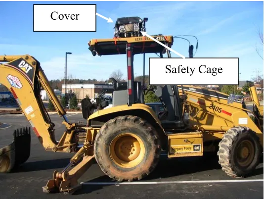
The Montana system should be located on a vehicle so that it does not block the driver or

operator view of the task being performed, nor interfere with the task-oriented functions

of the vehicle. For a backhoe, bulldozer, and front-end loader, the typical location for the

safety cage is on the roof of test vehicle. For a motor grader, the typical location for the

safety cage is on the hood. Figures 2.3 and 2.4 show the typical locations for a backhoe

and a motor grader, respectively.

Figure 2.2. Safety Cage for Montana Installation Rubber Pad Safety Cage

(34)

21

Figure 2.3. Safety Cage on a Backhoe

Figure 2.4. Safety Cage on a Motor Grader Safety Cage

Cover Cover

(35)

22

2.1.2 Exhaust Gases Sampling Hoses

Two sampling hoses are used in order to take exhaust gas samples from the tailpipe. An

exhaust gas sample for particulate matter is obtained from one sampling hose and for NO,

HC, CO, CO2, O2 from the other. The sampling hoses include a probe that is inserted

into the exhaust pipe. The probe assembly is secured to the tailpipe using an adjustable

metal hose clamp shown in Figure 2.5.

Figure 2.5. Attachment of Exhaust Gas Sampling Probes to the Tailpipe Exhaust Gas

Sampling Probes

Sampling hoses

Handles

(36)

23

The probe handles and the hoses should be located so that they are not in the path of hot

gases and so that they are not likely to get caught on any obstacles. The sampling hoses

should be secured to the equipment and there should be minimal slack in the line between

the tailpipe and the main unit. Each sampling hose is attached to the main unit through a

sample bowl. Figure 2.6 shows how a sampling hose connects to the main unit.

Figure 2.6. Attachment of the Sampling Hose to the Main Unit

The exhaust sampling probes should be inserted directly into the tailpipe in order to

obtain accurate tailpipe emissions. However, some construction equipment has a gap

between the muffler and tailpipe as shown in Figure 2.7. Fresh ambient air may enter the

tailpipe from this gap and dilute the pollutant concentration. In order to get accurate

emissions data, it is preferred not to have excess air enter the tailpipe and dilute the

exhaust gas. Main Unit Sample Bowl

(37)

24

A method that has been tried in the field and that appears to work well is to use several

layers of aluminum foil with two clamps for sealing the gap as shown in Figure 2.8. The

area where aluminum foil is used for sealing the gap is hot and care must be taken when

working with it.

Figure 2.7. Illustration of a Typical Gap between Muffler and Tailpipe

Figure 2.8. Sealing a Gap Using Aluminum Foil and Hose Clamps Hose Clamps Muffler

Tailpipe Gap

(38)

25

2.1.3 Sensor Array

A sensor unit is connected to the main unit to provide engine data. The sensor array is

composed of a manifold air boost pressure (MAP) sensor, engine speed sensor, intake air

temperature sensor, and sensor unit.

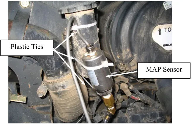
2.1.3.1 Manifold Air Boost Pressure Sensor

In order to measure MAP, a pressure sensor is installed on the engine. There is a port on

the engine after the turbocharger as shown in Figure 2.9. In a regular engine performance

check, this port is used for performance testing of the turbocharger. The MAP sensor

installation involves replacing Bolt “A”, shown in Figure 2.9, with a barb fitting, shown

in Figure 2.10. The data collection crew installs a barb fitting and connects it to the MAP

sensor. Plastic ties are used to route and secure the MAP sensor cable between the

engine and the main unit. Figure 2.11 shows the MAP sensor attached to a construction

vehicle engine. The MAP sensor provides manifold air pressure data for the computer of

the main unit through a cable that connects the sensor to the MAP port located in the

back of the main unit. The MAP sensor should be secured to adjacent engine parts using

(39)

26

Figure 2.9. Illustration of MAP Port

Figure 2.10. MAP Port on the Engine and a Barb Fitting Attached to the Port

MAP port and barb fitting MAP port

(40)

27

Figure 2.11. MAP Sensor after Installation

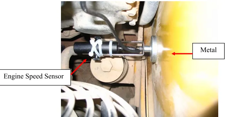
2.1.3.2 Engine Speed Sensor

The engine speed sensor must be installed at an adequate location in order to provide

accurate data. The engine speed sensor has strong magnetization to enable it to be

attached easily to metal materials as shown in Figure 2.12. Optical tape must be installed

on the pulley which is connected to the crankshaft. Thus, the location of the engine speed

sensor depends on the location of the optical tape. The optical tape reflects light from the

engine speed sensor. Based on this reflection, the engine speed sensor estimates engine

revolutions per minute. Thus, the correct placement of optical tape is essential to collect

engine speed data.

(41)

28

Figure 2.13 shows the location of optical tape on a pulley. Here are some suggestions for

the placement of the engine speed sensor:

1. Place in a position with no fans or other engine related obstacles

2. Place in a position with enough space to attach the sensor tightly

3. Place in a position within reachable length of the engine speed sensor cable

Figure 2.12. Magnetized Engine Speed Sensor Attached on the Metal Engine Speed Sensor

(42)

29

Figure 2.13. Engine Speed Sensor and Optical Tape

2.1.3.3 Intake Air Temperature Sensor

The engine intake air sensor needs to be installed in the intake air flow path. The sensor

has a metal part that can detect temperature. Installation of the intake air temperature

sensor is somewhat easy compared to the engine speed and MAP sensors. Using duct

tape or a plastic tie, one can fix the intake air temperature sensor near the intake air flow

where the MAP port is located. Figure 2.14 illustrates the location that the intake air

temperature sensor is installed on the engine of a bulldozer. The temperature sensor and

MAP port are close to each other, as shown in the figure. Engine Speed Sensor

Light from Engine Speed Sensor

Optical Tape

(43)

30

Figure 2.14. Installation of Intake Air Temperature Sensor

2.1.3.4 Sensor Unit

The sensor unit is the device which connects the intake air temperature and engine speed

sensors to the main unit. The sensor unit is protected by the box shown in Figure 2.15.

Plastic ties are used to secure the sensor unit to the construction vehicle. If the sensor

unit cannot be affixed to the vehicle using plastic ties, duct tape can usually be used to

secure the sensor unit.

Intake Air Temperature Sensor

Plastic Ties

(44)

31

Figure 2.15. Sensor Unit on a Bulldozer

2.1.4 External Power Source

The main unit of the Montana system needs at least 12 volts and 4 to 6 amps of direct

current electricity. Although it is often possible to obtain such power from the vehicle,

the use of external batteries as a power source avoids putting additional load on the

engine. Also, using batteries avoids an unintended shutdown of the Montana system if

the vehicle operator inadvertently turns off the engine. When moving these batteries

from the laboratory to the job site, it is important to tape all of the connectors using duct

tape to avoid a short circuit. Also, the batteries should be placed into an appropriate

container to protect them from being impacted. When installed, the batteries should be

tied down to the body of the vehicle using a strap as shown in Figure 2.16. A rubber pad

is used to reduce vibration from the vehicle. Each battery can operate the Montana

system for 4 to 5 hours.

Box

Sensor Unit

(45)

32

Figure 2.16. External Battery Setup for Montana System Power Source

2.1.5 Measurement Instrument Pre-test

After setup of the safety cage, exhaust gas sampling hoses, sensors, and batteries, the next

step is to make sure that the main unit of the Montana system obtains valid data from the

engine sensors. Generally, there is no problem with the MAP and intake air temperature

sensors. However, the engine speed sensor often needs to be tested several times in order

to find the best way to set up the sensor and the optical tape. If the Montana system

cannot obtain engine speed data, or if the engine speed values fluctuate rapidly, there is a

need to re-install the engine speed sensor. If the Montana system reads engine RPM data

properly after the re-installation of the engine speed sensor, the pre-installation procedure

is done. Otherwise, the pre-installation testing should be repeated until the Montana

system can read RPM data properly.

Strap Rubber Pad

(46)

33

2.1.6 Calibration of Montana System

Because the NO and O2 sensors deteriorate with use, they have to be calibrated between

once a week and once a month during data collection. To do so, after pre-installation, the

main unit of the Montana system will be brought to the laboratory and calibrated. When

performing calibration, the instrument has to be warmed up for forty-five minutes. The

calibration procedures of the Montana system are detailed in the user’s manual (Clean

Air Technology Inc).

The calibration gas mixture recommended when data is to be collected from diesel

engines is 200 ppm propane (C3H8), 0.5 vol-% carbon monoxide (CO), 6.0 vol-% carbon dioxide (CO2) and 300 ppm nitric oxide (NO). There is no O2 in the calibration mixture

gas. During calibration, neither of the gas analyzer benches should detect O2. If the O2

concentration is higher than zero, then some leakage may have occurred inside the

(47)

34

2.2 Installation

The difference between pre-installation and installation is that installation is done before

the vehicle operator starts working on the test day, whereas pre-installation is done the

day before the test. The data collection crew arrives at the job site one hour earlier than

construction workers. When the installation is done, the Montana system is ready to

collect data from the construction vehicle.

Some of the major components of the Montana system are already pre-installed on the

construction vehicle as described previously in Section 4.1. On the test day, the

installation procedures focus on set up of the main unit of the Montana system, the

Geographical Positioning System (GPS), the video capture instrument (camcorder), and

(48)

35

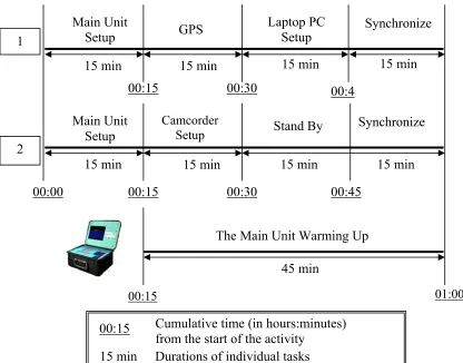
The main unit has to warm up for forty-five minutes before collecting data. The data

collection crew can install other instruments while the main unit is warming up. Two

people are needed to operate the camcorder and the laptop computer separately during

data collection. Figure 2.17 shows the timeline for installation procedures performed by

two people. The installation procedures take one hour to finish. As mentioned before,

the time period may vary due to the ambient condition and the height of construction

equipment. Table 2.4 shows the typical installation time period and range for a backhoe,

(49)

36

Table 2.3 Installation Checklist Form

Installation Procedure Checklist Main Unit

– Locate the main unit in the safety cage – Connect the engine sensors to the main unit – Warm up for forty-five minutes

Geographical Positioning System

– Affix the GPS receiver on the top of the construction vehicle

– Connect the cable from GPS to the main unit – Secure the cable to the safety cage

Camcorder

– Connect the camcorder with the tripod – Slide the POWER switch to turn on the

camcorder Laptop Computer

– Turn on the laptop computer – Open Microsoft Excel – Run the Visual Basic Macro Synchronize

(50)

37

Figure 2.17 Timeline for Installation Procedures Performed by Two Persons

Table 2.4 Typical Time Period and Range for Installation Based on Equipment Type

Installation Time Period Equipment Type

Typical Range

Backhoe 1 hr 00 min

Motor Grader 1 hr 00 min 1 hr 00 min to 1 hr 50 min

Front-End Loader 1 hr 00 min 1 hr 00 min to 1 hr 50 min 15 min Main Unit Setup 00:00 00:15 GPS 15 min Laptop PC Setup 15 min 00:30 00:4 00:15

The Main Unit Warming Up

45 min 01:00 15 min Main Unit Setup Camcorder Setup 15 min 00:15 00:30 Synchronize Stand By 15 min

Durations of individual tasks 00:15 Cumulative time (in hours:minutes)

from the start of the activity 15 min

15 min 15 min

Synchronize

00:45 2

(51)

38

2.2.1 Main Unit

On the test day, when the data collection crew gets to the construction site, the first step

is to install the main unit of the Montana system. Flexible rubber pads and foam rubber

are placed underneath the main unit of the Montana system in order to reduce vibration

from the construction vehicle as shown in Figure 2.2. Moreover, the main unit should be

fastened with the safety cage using plastic ties. After the installation is done, the main

unit should be warmed up for forty-five minutes. During this period, the data collection

crew can set up the GPS, the camcorder, and the laptop computer.

2.2.2 Geographical Positioning System

The Global Positioning System (GPS) is a device to determine the construction vehicle’s

position by triangulating distances from satellites. This device has a strong magnetic tape

under the receiver to hold it in place. Thus, the receiver can be affixed to a steel surface

on the vehicle. The recommended location of the GPS receiver is on the roof of the

vehicle so that it has the best signal from satellites. Figure 2.18 shows a picture of the

(52)

39

Figure 2.18 Trimble GPS Receiver

2.2.3 Camcorder

A camcorder with a tripod is used to record the activity pattern of the construction

equipment. The camcorder should be installed in a safe place that is not too close to the

work zone. A member of the data collection crew operates the camcorder and makes a

video recording of the work activities. For example, as a motor grader often moves

around a large area, the data collection crew should follow the motor grader and record

the work activities. For other construction vehicles, such as backhoes and bulldozers, the

data collection crew may stay in one place and record the video without moving the setup.

(53)

40

2.2.4 Laptop Computer

A laptop computer with Microsoft Excel is used to record data regarding the modal

activity of the vehicle. A Visual Basic program has been prepared for recording modal

activity. The program is running during data collection. A member of the data collection

crew records modal activity using the keyboard. The laptop computer can be used for

three hours. Its use is limited by battery capacity. It is recommended that the laptop

computer be charged every two hours. The data collection crew uses the cigarette lighter

in a passenger car to provide the power of laptop computer. Thus, data collection will not

be interrupted when the laptop computer is recharging.

2.2.5 Synchronizing the Main Unit, Camcorder, and Laptop Computer

The data collection crew synchronizes the time of the camcorder and the laptop computer

based on the main unit of the Montana system. Because data analysis is based on

second-by-second data, if the time shown on the main unit, laptop computer, and camcorder are

different, it would pose a challenge to data analysis. Thus, it is important to synchronize

these instruments before data collection. Figure 2.19 shows the synchronization of

(54)

41

Figure 2.19 Synchronization of the Camcorder and the Laptop Computer

2.3 Data Collection

On the day that data is to be collected, the researchers typically arrive at the construction

site approximately two hours before data collection is to begin in order to prepare the

equipment. There are six primary tasks to be completed in the data collection process.

These are:

1. Install and use the Montana System

2. Prepare and use the laptop computer

3. Prepare and use the video camera

4. Assess and record the field conditions

5. Collect and record equipment data

6. Archive data

Camcorder

(55)

42

When the installation is completed and the Montana system has warmed up for forty-five

minutes, the Montana system can be used to collect data from construction equipment.

During data collection, the camcorder will make a video recording of the construction

vehicle and the laptop computer is used to record the modal activity. This section

describes the field procedures during data collection.

After the main unit has warmed up for forty-five minutes, it is ready for collecting data.

One person uses the camcorder to record the work pattern of the construction vehicle. A

second person records modal activities using the laptop computer. Approximately every

thirty minutes, it is important to check the main unit of the Montana system to verify that

it is working properly. Based on experience, there are various types of problems that can

be encountered during field data collection. Many of these can be solved on site if they

are detected or identified. These problems and their solutions are described in another

appendix. The checklist for data collection is shown in Table 2.5. Figure 2.20 shows the

(56)

43

Table 2.5 Data Collection Checklist Form

Data Collection Checklist Montana System Measurement

– Start a new file for data collection Camcorder

– Make a video recording of the construction vehicle

Laptop Computer

– Record modal activities of the construction vehicle

(57)

44

Figure 2.20 Timeline for Data Collection Procedures

2.4 Decommissioning

When data collection activity is finished, each instrument and sensor should be removed

or disconnected from the construction equipment. It typically takes thirty minutes to

finish the decommissioning. All equipment is brought to the laboratory for cleanup after

decommissioning.

30 min Camcorder

00:00 00:30

00:00

Montana System Measurement 40 min

Laptop Computer

00:00 00:40

5 min Periodic Checking 40 min 30 min Stand By 5 min

Laptop Computer …..

…..

(58)

45

The decommissioning procedures can be completed by either one or two persons. Table

2.6 shows the checklist of decommissioning procedures. The timeline for

decommissioning by one person is shown in Figure 2.21. Figure 2.22 depicts the

timeline for two persons. Overall it takes one person about one hour and ten minutes to

complete decommissioning and it takes 2 people about 35 minutes.

Table 2.6 Decommissioning Checklist Form

Decommissioning Checklist Main Unit

– Disconnect the sampling hoses in the back of the main unit

– Disconnect the sampling bowl – Disconnect the cables

– Disconnect the GPS – Disconnect the keyboard

– Bring the main unit to the laboratory Safety Cage

– Dismantle the safety cage

– Bring the safety cage to the laboratory Exhaust Gases Sampling Hoses

– Disconnect the exhaust gases sampling hoses from the tailpipe

– Put the exhaust gases sampling hoses into a plastic bag

(59)

46 Table 2.6. Continued.

Sensor Unit

– Disconnect the cable from sensor unit to the engine sensors

– Put the sensor unit into the box

– Bring the sensor unit to the laboratory MAP Sensor

– Disconnect the MAP sensor – Put the MAP sensor into the box

– Bring the MAP sensor to the laboratory Engine Speed Sensor

– Disconnect the engine speed sensor – Put the engine speed sensor into the box – Bring the engine speed sensor to the laboratory Intake Air Temperature Sensor

– Disconnect the intake air temperature sensor – Put the intake air temperature sensor into the box – Bring the intake air temperature sensor to the

laboratory External Power Sources

– Disconnect external power sources – Tape all the connector using duct tape – Place the battery into a container – Bring the battery to the laboratory Geographical Positioning System

– Disconnect geographical positioning system – Bring the GPS to the laboratory

(60)

47 Table 2.6. Continued.

Video

– Turn off the camcorder

– Put the camcorder into the bag

– Bring the camcorder to the laboratory Laptop Computer

– Save the Excel file

– Turn off the laptop computer

– Put the laptop computer into the bag

– Bring the laptop computer to the laboratory Wrap Up

– Pick up tools and put into the toolbox

Figure 2.21 Timeline for Decommissioning Performed by One Person 5 min Main Unit 5 min Temperature Sensor 00:00 Sampling Hoses 5 min Sensor Unit 5 min MAP Sensor 10 min RPM Sensor 10 min

00:15 00:20 00:30 00:40

00:40 00:45

External Power 5 min 00:50 5 min GPS 00:55 Camcorder 01:00 5 min Laptop

PC Wrap Up 00:10

00:05

from the start of the activity

30 min Safety

Cage

5 min

01:05 01:10

(61)

48

Figure 2.22 Timeline for Decommissioning Performed by Two Persons

2.4.1 Main Unit

The decommissioning of the main unit includes removing the safety cage and the main

unit of the Montana system from the construction vehicle. First, the cables and the

sampling hoses should be disconnected from the main unit. The main unit is usually

installed on the roof of cab. The unit must be taken out of the safety cage and lower it to

the ground. The best way to do this is if one person climbs to the roof and transfers the

main unit to the other person.

MAP Sensor Main Unit

5 min 5 min Safety

Cage

RPM Sensor

10 min 5 min 5 min

Sampling

Hose Sensor Unit External Power

Laptop PC

5 min 5 min

5 min GPS 5 min Cam-corder Wrap Up 5 min Wrap Up

00:05 00:10 00:20 00:25 00:30

00:35

00:00 00:10 00:20 00:30

(62)

49

2.4.2 Exhaust Gases Sampling Hoses

The decommissioning of sampling hoses is not difficult and takes only five minutes to

finish. The plastic ties should be removed first. The sampling probes should be

disconnected from the tailpipe. The sampling probes are very dirty after a full day of

testing. Thus, the sampling hoses should be stored in a plastic bag for their return to the

laboratory.

2.4.3 Engine Sensors

The decommissioning of engine sensors includes disconnection of the sensor unit, the

MAP sensor, the intake air temperature sensor, and the engine speed sensor. Even after

the engine of a construction vehicle has been shut off, the engine temperature can still be

very high. For safety, the data collection crew usually starts decommissioning the

sensors no sooner than ten minutes after the engine stops. Even then extreme care must

(63)

50

2.4.4 External Power Source, Geographical Positioning System, Camcorder, and Laptop Computer

The decommissioning of the batteries, the GPS, the camcorder, and the laptop computer

is the last step. The connectors of the batteries should be covered with duct tape. Then,

the battery is placed into an appropriate container to protect the battery from being

impacted. After the GPS is disconnected from the main unit, it should be put into the

storage box. The camcorder should be shut down before decommissioning. The

camcorder and tripod will be returned to the laboratory. Prior to decommissioning the

laptop computer, the Excel file of modal activities should be saved first. The laptop

computer will be shut down and returned to the laboratory. It is important to make sure

that all instruments are brought to the laboratory.

2.5 Cleanup after Data Collection

Each of the main parts of the main unit should be cleaned up: outside the box, the gas

analyzer, and the computer. Cleanup procedures for other instruments are also identified

(64)

51

Table 2.7 Cleanup Checklist Form

Cleanup Checklist Main Unit

– Clean up outside the box – Clean up the gas analyzers – Clean up the computer Safety Cage

– Remove dust from the safety cage – Clean up the rubber pads

Exhaust Gases Sampling Hoses – Remove dust from the hoses – Clean up the sampling probe

– Clean up the sampling gas and PM bowl – Replace the filter for the gas sampling bowl as

needed Engine Sensors

– Remove dust from the MAP sensor

– Remove dust from the engine speed sensor – Remove dust from the intake air temperature

sensor

– Remove dust from the sensor unit External Power Source

– Remove dust from the batteries – Recharge the batteries

(65)

52 Table 2.7 Continued.

Camcorder

– Remove dust from the camcorder – Remove dust from the tripod – Download the video file Laptop Computer

– Remove dust from the laptop computer – Remove dust from the keyboard

– Download the Excel file of modal activities

2.5.1 Main Unit

The following text explains the sequential steps that are necessary and critical for

cleaning the Montana after data collection. These procedures are to be initiated after

every field data collection operation is completed. Figure 2.23 shows the Montana

(66)

53

Figure 2.23 Parts of the Montana Addressed in the Cleaning Procedure

2.5.1.1 Outside the Box

The procedures for cleaning the box are listed below:

1. Close the top panel of the main unit

2. Ensure that all ports located on the back panel of the main unit are unplugged and

that all caps are closed

3. Use a dust remover to clean the outside of case

4. Leave the main unit open for 3~5 minutes to allow air circulation to dry any

accumulated moisture

5. Open the top panel of the main unit

6. Clean the power and computer panel using a dust remover

7. Leave the main unit open for 3~5 minutes to allow air circulation to dry any

accumulated moisture Computer

Power Panel

Main Unit

Cables

Gas Analyzers Computer