HIGHLIGHTED ARTICLE INVESTIGATION
Adaptive Fixation in Two-Locus Models of
Stabilizing Selection and Genetic Drift
Andreas Wollstein1and Wolfgang Stephan1 Section of Evolutionary Biology, Department of Biology II, University of Munich, D-82152 Planegg-Martinsried, Germany
ABSTRACTThe relationship between quantitative genetics and population genetics has been studied for nearly a century, almost since the existence of these two disciplines. Here we ask to what extent quantitative genetic models in which selection is assumed to operate on a polygenic trait predict adaptivefixations that may lead to footprints in the genome (selective sweeps). We study two-locus models of stabilizing selection (with and without genetic drift) by simulations and analytically. For symmetric viability selection wefind that 16% of the trajectories may lead tofixation if the initial allele frequencies are sampled from the neutral site-frequency spectrum and the effect sizes are uniformly distributed. However, if the population is preadapted when it undergoes an environmental change (i.e., sits in one of the equilibria of the model), thefixation probability decreases dramatically. In other two-locus models with general viabilities or an optimum shift, the proportion of adaptivefixations may increase to.24%. Similarly, genetic drift leads to a higher probability offixation. The predictions of alternative quantitative genetics models, initial conditions, and effect-size distributions are also discussed.
Q
UANTITATIVE genetics assumes that selection on an adaptive character involves simultaneous selection at multiple loci controlling the trait. This may cause small to moderate allele-frequency shifts at these loci, in particular when traits are highly polygenic (Barton and Keightley 2002). Therefore, adaptation does not require new muta-tions in the short term. Instead, selection uses alleles found in the standing variation of a population. Genome-wide polymorphism data and association studies suggest that this quantitative genetic view is relevant (Pritchard and Di Rien-zo 2010; Pritchardet al.2010; Mackayet al.2012).Different types of selection on a trait, such as directional, stabilizing, or disruptive selection, modify the genetic composition of a population and favor either extreme or intermediate genotypic values of the trait. In this study we focus on stabilizing selection, which drives a trait toward a phenotypic optimum. Many models of this common form of selection have been analyzed. The central question in all these studies has been whether stabilizing selection can explain the maintenance of genetic variation. This is
considered an important question, as it has been known for long that stabilizing selection exhausts genetic variation (Fisher 1930; Robertson 1956), yet quantitative traits ex-hibit relatively high levels of genetic variation in nature (Endler 1986; Falconer and Mackay 1996; Lynch and Walsh 1998).
Here we ask a different question, namely how much adaptive evolution is predicted by quantitative genetic models of stabilizing selection? In contrast to quantitative genetics, in population genetics and genomics our under-standing of the genetics of adaptation has revolved in recent years around the role of selective sweeps,i.e., signatures of positive directional selection in the genome. The model un-derlying this population genetic view of adaptation is that of the hitchhiking effect developed for sexual species by Maynard Smith and Haigh (1974). The hitchhiking process describes how the fixation of a beneficial allele (starting from very low frequency) affects neutral or weakly selected variation linked to the selected site. For single and recurrent advantageous alleles appearing in a population, the model has been further developed by Kaplanet al.(1989), Stephan
et al.(1992), Stephan (1995), and Barton (1998). Later this model was generalized to sweeps from standing variation or soft sweeps taking into account that sweeps may also occur if the initial frequency of the beneficial allele is not very low (Innan and Kim 2004; Hermisson and Pennings 2005).
Copyright © 2014 by the Genetics Society of America doi: 10.1534/genetics.114.168567
Manuscript received March 31, 2014; accepted for publication July 20, 2014; published Early Online August 4, 2014.
1Corresponding authors: LMU München, Biozentrum Martinsried, Großhaderner
Yet, despite its simplicity, the use of the hitchhiking model was quite successful in recent years in detecting evidence for positive directional selection in the genomes of plant and animal species. Typically, many studies of pop-ulations with large effective sizes have revealed numerous genes or gene regions showing selective footprints (reviewed in Stephan 2010). The detection of such foot-prints is based on statistical tests that utilize several features of the hitchhiking model such as reduced variation around the selected site and shifts in the neutral site-frequency spec-trum (Kim and Stephan 2002; Nielsen et al.2005; Pavlidis
et al. 2010). However, it is remarkable that none of these tests incorporates phenotypic information. If functional studies were performed to reach an understanding of the effects of selection, they were done in most cases onlypost hoc, after a gene or gene region has been identified by a sweep.
Recent theoretical work has addressed the question whether and to what extent the quantitative and population genetics views of adaptation are compatible with each other. For instance, the following question was asked: Can the quantitative genetics models of stabilizing selection also be used to predict observed levels of selectivefixations? Chevin and Hospital (2008) presented a model for the footprint of positive directional selection at a quantitative trait locus (QTL) in the presence of a fixed amount of background genetic variation due to other loci. This approach is based on Lande’s (1983) model that consists of a locus of major effect on the trait and treats the remaining loci of minor effect as genetic background. This analysis predicts that QTL of adaptive traits under stabilizing selection exhibit patterns of selective sweeps only very rarely. de Vladar and Barton (2011, 2014) studied a polygenic character un-der stabilizing selection, mutation, and genetic drift. They found sweeps after abrupt shifts of the phenotypic optimum, without quantifying how often such signatures occurred. Fur-thermore, Pavlidis et al. (2012) analyzed a classical multi-locus model with two to eight loci controlling an additive quantitative trait under stabilizing selection (with and with-out genetic drift). Using simulations, they showed that multi-locus response to selection often prevents trajectories from going to fixation, particularly for the symmetric viability model. They also found that the probability of fixation strongly depends on the genetic architecture of the trait. To understand these results in greater depth, we present here an analysis of the two-locus model of an adaptive trait under stabilizing selection and drift. This model is suffi -ciently simple that analytical approximations can be used to back up the simulations. We concentrate on the case of weak selection. Given that we are interested in a comparison between quantitative and population genetics and selection coefficients estimated in molecular population genetics are generally small (,1021), this parameter range appears to be justified (Orr 2005; Turchin et al.2012). We show that in this realm quasi-linkage equilibrium (QLE) approximations are possible. Furthermore, we address the question of initial
conditions, a subject that was neglected in all of the above-mentioned studies. These, however, are important as the two- and multilocus models of stabilizing selection have generally multiple stable equilibrium states and hence vari-ous basins of attraction, which may make the ensuing dy-namics sensitive to the initial conditions.
Models
Symmetricfitness model
We consider two loci with two alleles each, A1 and A2 at locus AandB1andB2at locusB. The effects of the alleles
A1,A2,B1, andB2on a quantitative trait are21 2gA;
1 2gA;2
1 2gB;
and 12gB; respectively. Assuming additivity, the effects of the gametesA1B1,A1B2,A2B1, andA2B2are 21
2ðgAþgBÞ;
21
2ðgA2gBÞ; 12ðgA2gBÞ;and12ðgAþgBÞ;respectively. The
resulting genotypic values are given by
B1B1 B1B2 B2B2
A1A1
A1A2
A2A2 0
@2g2Ag2BgB 20gA 2gAgþB gB
gA2gB gA gAþgB
1
A: (1)
Without loss of generality, we assume 0 # gB # gA; i.e.,
locusAis the major and locusBthe minor locus.
Under sufficiently weak selection (and/or for sufficiently small genotypic effects), it may be assumed that the trait is under quadratic stabilizing selection;i.e., the relativefitness
w(G) of individuals with genotypic valueGis
wðGÞ ¼12sG2; (2)
wheresis the selection coefficient. The relativefitnesses of all genotypes are then given by
B1B1 B1B2 B2B2
A1A1
A1A2
A2A2 0
@1122dc 121b 1122ac
12a 12b 12d
1
A; (3)
wherea¼sðgA2gBÞ 2;
b¼sg2A;c¼sg2B;andd¼sðg AþgBÞ
2
(Bürger 2000, p. 204). Neglecting mutation, the ordinary differential equations (ODEs) determining the dynamics of the system can then be written as
_
x1¼x1ðw12wÞ2rD;
_
x2¼x2ðw22wÞ1rD;
_
x3¼x3ðw32wÞ1rD;
_
x4¼x4ðw42wÞ2rD;
(4)
between 0 and 0.5. The marginalfitnesseswi(i= 1,..., 4) of the gametes (Bürger 2000, p. 51) are
w1¼12dx12bx22cx3;
w2¼12bx12ax22cx4;
w3¼12cx12ax32bx4;
w4¼12cx22bx32dx4;
(5)
and the meanfitness of the population is
w¼12dx21þx242ax22þx3222bðx1x2þx3x4Þ
22cðx1x3þx2x4Þ: (6)
The equilibria of the system of ODEs (4) and their stability properties are identical to those of the correspond-ing discrete-time model, which has been studied by Gavrilets and Hastings (1993) and Bürger and Gimelfarb (1999). As reviewed in Bürger (2000, pp. 204-208), there are four possible types of equilibria: (i) four monomorphic equilibria (henceforth also called corner equilibria) corresponding to thefixation of the gametesA1B1,A1B2,A2B1, andA2B2; (ii) two edge equilibria with the major locus polymorphic and the minor locus fixed; (iii) a symmetric (internal) equilib-rium for which both loci are polymorphic, and (iv) two unsymmetric equilibria. The conditions for the existence of these equilibria, their explicit expressions, and their local stability properties are summarized in Bürger (2000, pp. 205–208).
QLE approximation: To gain insight into the qualitative behavior of the ODEs (4), it is convenient to reduce the system from three to two dimensions. This is possible if, in addition to weak selection, linkage is sufficiently loose (relative to epistasis). This is the so-called QLE assumption, which was introduced by Kimura (1965a). In other words, we transform the gamete frequenciesxi(i= 1,...,4) into the frequenciesp=x1+x2andq=x1+x3of the allelesA1and
B1, respectively, and introduce linkage disequilibriumD as the third new variable. Then we treat the latter as a fast variable on the time scale of changes in p and q. The xi
can be expressed by the new variables as
x1¼pqþD;
x2¼pð12qÞ2D;
x3¼ ð12pÞq2D;
x4¼ ð12pÞð12qÞ þD:
(7)
Next, following Kimura we use Z=x1x4/x2x3as a mea-sure of LD. Then with the help of the ODEs (4), the time derivative of Zcan be written as (Crow and Kimura 1970, p. 198)
1
Z dZ
dt¼E2rD
X4
i¼1
1
xi;
(8)
where E=w1 2w2 2w3+w4 measures the strength of epistasis. Note that in our case
E¼ 22sgAgB¼const:,0: (9)
In the QLE, Equation 8 can be evaluated to give the leading-order term
D¼E
rpqð12pÞð12qÞ: (10)
By insertingD into the variablesxiin (7), the reduced sys-tem of ODEs can be written in the form
_
p¼sg2Apð12pÞð122pÞ þ2sgAgBpð12pÞð122qÞ þOs2r;
_
q¼sg2Bqð12qÞð122qÞ þ2sgAgBqð12qÞð122pÞ þOs2r:
(11)
The local stability properties of the equilibria of Equa-tions 11 are quite similar to those of the original system (4). The two corner equilibria ^p¼^q¼0 and ^p¼^q¼1 are al-ways unstable, as the respective eigenvalues are alal-ways pos-itive. The biological explanation would be that the extreme phenotypes are selected against when the optimum is the double heterozygote. The corner equilibria ^p¼0; ^q¼1 and
^
p¼1; ^q¼0 are stable if the conditiongA/2,gB,gAholds.
Edge equilibria exist for^q¼0; ^p¼1=2þgB=gA;and for
^
q¼1; ^p¼1=22gB=gA (Bürger 2000, p. 205). The
stabil-ity condition is identical to that of the full system, as for 0,gB,gA=2 both edge equilibria are stable.
The main difference from the full system (4) is that the internal symmetric equilibrium is always unstable. This can be seen by linearizing the reduced system about
^
p¼q^¼1=2. Neglecting higher-order terms ins, the Jaco-bian of (11) becomes
0 B B B @
2sg2A
2 sgAgB
2sgAgB sg2B 2
1 C C C
A; (12)
with its eigenvalues
l1¼1
4s
2g2
A2g2B2
ffiffiffiffiffiffiffiffiffiffiffiffiffiffiffiffiffiffiffiffiffiffiffiffiffiffiffiffiffiffiffiffiffiffiffiffiffiffiffiffiffi
g4
Aþ14 g2Ag2Bþg4B
q
;
l2¼
1 4s
2g2
A2g2B1
ffiffiffiffiffiffiffiffiffiffiffiffiffiffiffiffiffiffiffiffiffiffiffiffiffiffiffiffiffiffiffiffiffiffiffiffiffiffiffiffiffi
g4
Aþ14 g2Ag2Bþg4B
q
:
(13)
Thus, for ^p¼^q¼1
2the eigenvalues of this matrix have
op-posite signs, showing that this equilibrium point is unstable. In fact, since the eigenvalues are real,^p¼^q¼1
2 is a saddle
point. The two separatrices of this saddle divide the pq
The parameter ranges of stability for the different systems depend on gB/gA and r/s. Inner stable equilibria
exist only in the full system (4). For r/s sufficiently large, the stability properties of the edge equilibria are equivalent in the full and the QLE system. Monomorphic equilibria are also qualitatively equal in both systems.
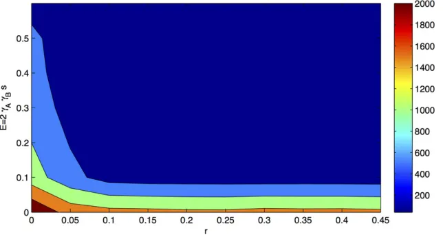
Accuracy of the QLE approximation: We estimated the range of parameter values for which we obtain a reasonably good QLE approximation of the two-locus model. We generated a set of random parameter values as described in Table 1 and initial conditions for which we estimated the trajectory from the full system and the QLE system. Then we compared both trajectories by calculating the mean relative error using the distance
dðtÞ ¼p9ðtÞ2pðtÞ p9ðtÞ þ
q9ðtÞ2qðtÞ q9ðtÞ ;
summed over all times t. Here p9ðtÞ ¼x1ðtÞ þx2ðtÞ and
q9ðtÞ ¼x1ðtÞ þx3ðtÞ denote the trajectories from the full model and p(t) and q(t) are the trajectories of the QLE approximation.
In Figure 1 it can be seen that for increasing recombina-tion rates the mean error is ,5%, which corresponds to a threshold of 23 (blue to dark blue areas in Figure 1A and green to yellow in Figure 1B). For example, assuming 2sgAgB = 0.04 would require a recombination rate above
0.07 to achieve an approximation of the two-locus model with a relative error,5%. Thus, when assuming a relatively low selection coefficient of 0.01, the effects could be mod-erately high, such as gA = gB = 1.5. For many parameter
ranges of interest this is a sufficiently good approximation. Figure 1B demonstrates that the ratio of the effects has only a marginal impact on the quality of the approximation.
Generalizing the symmetricfitness model
We have studied two generalizations of the symmetric
fitness model. First, in thegeneralfitness model we relaxed the restrictions on the relations of allelic contributions by allowing for arbitrary values of the effectsgA1,gA2,gB1, and
gB2for the allelesA1,A2,B1, andB2, respectively. However,
by assuming that the absolute values of gA1 and gA2 are
equal or larger than those of gB1andgB2, we further
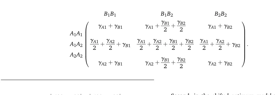
con-sider locusAas the major and locusB as minor locus, and the phenotypic optimum is again 0. In this case the geno-typic values are
Second, in the shifted optimum model we consider the quadratic optimum model with an arbitrary position u of the optimum, yet assign the effects as in the symmetric fi t-ness model. Note that in both cases the genotypicfitnesses may no longer conform to the symmetric viability model.
General fitness model:We established the ODEs in accor-dance to those of system (4) and investigated this model numerically. Furthermore, we derived the ODEs using the QLE approximation as
_ p¼1
4sðgA22gA1Þpð12pÞ ð3gA2þgA1Þ22ðgA22gA1Þp þ4ðgB22ðgB22gB1ÞqÞ
þOs2r; _
q¼1
4sðgB22gB1Þqð12qÞ ð3gB2þgB1Þ22ðgB22gB1Þq þ4ðgA22ðgA22gA1ÞpÞ
þOs2r:
(15)
Thus, if the effectsgijare chosen as in the symmetricfitness
model, Equations 15 reduce to Equations 11. Furthermore, if the parameter values follow constraints similar to those in the symmetric fitness model, the equilibrium structure of (15) is similar to that of (11). In particular, if the absolute values of the effects of both loci are comparable, but their
Table 1 Parameter values used for simulations
Parameter Range Condition
gA Uniform(0, 2)
gB Uniform(0, 2) gB#gA
r Uniform(0, 0.5)
s Uniform(0, 0.1)
B1B1 B1B2 B2B2
A1A1
A1A2
A2A2 0 B B B B B B B @
gA1þgB1 gA1þgB1
2 þ
gB2
2 gA1þgB2
gA1
2 þ
gA2
2 þgB1
gA1
2 þ
gA2
2 þ
gB1
2 þ
gB2
2
gA1
2 þ
gA2
2 þgB2
gA2þgB1 gA2þgB1
2 þ
gB2
2 gA2þgB2
1 C C C C C C C A
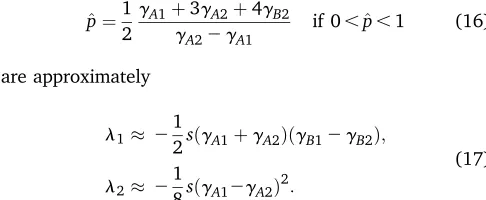
signs are opposite for each locus, the corner equilibria (1, 0) and (0, 1) are locally stable and the other two are unstable. If the absolute values of the effects of the major locus are sufficiently large relative to those of the minor locus, wefind again two edge equilibria. For instance, the eigenvalues of ð^p;0Þwith
^ p¼1
2
gA1þ3gA2þ4gB2
gA22gA1 if 0,^p,1 (16)
are approximately
l1 21
2sðgA1þgA2ÞðgB12gB2Þ;
l2 2
1
8sðgA12gA2Þ
2:
(17)
Hence, ð^p;0Þ is locally stable if the parametersgA1 +gA2
andgB1–gB2have the same sign. Finally, the interior
equi-librium ^p¼^q¼1
2 exists and remains a saddle point if and
only if gA1 +gA2 +gB1 +gB2 = 0. Under more general
conditions, however, this equilibrium does no longer exist, as we show in our simulations (Table 2).
Shifted optimum model:Here we use thefitness function
wðGÞ ¼12sðG2uÞ2 (18)
for individuals with genotypic value G (Bürger 2000, p. 213). Then assuming that the effects follow those used in the symmetric fitness model, the ODEs under the QLE ap-proximation are
_
p¼sg2Apð12pÞð122pÞ þ2sgAgBpð12pÞð122qÞ 22sgAupð12pÞ þO
s2r;
_ q¼sg2
Bqð12qÞð122qÞ þ2sgAgBqð12qÞð122pÞ 22sgBuqð12qÞ þO
s2r:
(19)
The equilibrium structure of this model is discussed in Bür-ger (2000, pp. 213–214) as a function ofu.0. Foru
suf-ficiently small, either two stable corner equilibria or two stable edge equilibria exist, depending on the ratio gB/gA.
For u$gA212gBthe corner equilibrium (0, 1) becomes
un-stable and the un-stable edge equilibrium
^
p¼0 and ^q¼1
2þ
gA gB 2
u
gB (20)
arises. For u$gAþ12gB both loci are under directional
se-lection driving the most extreme gamete tofixation.
Simulations
Simulation settings were kept identical throughout this section. The model parameters were drawn according to Table 1. Initial gamete frequencies were produced under the assumption of no initial LD with the constraintP4i¼1xi¼1:
Furthermore, initial conditions of the gamete frequencies were drawn from allele frequencies that were distributed as the standard neutral site-frequency spectrum (i.e., for constant population size). To do so, we sampled the locus frequencies from the neutral site-frequency spectrum
(Grif-fiths and Tavaré 1998, Equation 1.3) for a large sample size (n = 50). This choice of initial conditions is biologically more plausible than the random initial frequency values used in Pavlidiset al.(2012). The initial gamete frequencies are in our case clustered near the corner equilibrium (E8) such that the frequencies of both allelesA1andB1are low. For each parameter set the simulation was run for 10,000 generations forward in time. In total, 10,000 simula-tions were produced. Various environmental settings were analyzed: (i) a constant environment under which weak stabilizing selection is acting on the trait, (ii) a constant environment with strong stabilizing selection, (iii) a change in the environmental parameter values describing stabilizing selection (i.e., effects and selection coefficient), (iv) a change
in the optimum of the trait, and (v) a generalfitness model as described above. For each environmental setting we stud-ied the equilibrium structure of the dynamical system under uniformly distributed parameter values. In addition, to be biologically more realistic, we used specific distributions for some parameters (e.g., effect sizes).
Deterministic simulations
For a given parameter set we solved the ODEs (4) using the
“ode23s”command in Matlab (v. 6). We refer to the param-eter setting as constant environment when the paramparam-eters of the symmetricfitness model arefixed during evolution. In the following, we report the percentage of trajectories that converge to a certain equilibrium point of the symmetric model defined by Bürger (2000, p. 205).
First, in the case of a trait under stabilizing selection according to the symmetric model (constant environment) and weak selection (s,0.1), we observed that only 2% of all simulations end up in a symmetric, polymorphic equilib-rium (E1, see Table 2). About 5% of all trajectories reached one of the unsymmetric equilibria (E2 + E3). Edge equilib-ria with locus A polymorphic and a loss at locus B were reached in 35% of the cases (E4), whereas only 1% of the runs ended atBwithApolymorphic (E5). We also observed that more trajectories (31%) approach the corner where
fixation occurs atA(and loss atB, E6) compared tofixation at B (and loss atA, E7) (11%). The higher proportion of
fixations atA(rather than locusB) is due to the fact thatA
has been chosen as major locus. Thus, in total 42% of the trajectories were fixed at locus A(E6) or B (E7), whereas 43% converged to the polymorphic equilibria (E1–E5). Note that the proportions of trajectories approaching the equilib-ria E1–E9 do not add up to 100%. A substantial percentage (14%) did not converge within the simulated 10,000
generations, particularly when the effects and selection
coef-ficients are close to zero, and a small percentage of2% could not be assigned exactly to one of the possible equilib-rium points due to numerical errors in the approximation of the trajectory or unreached equilibrium states. Furthermore, some corner equilibria (E8 and E9) are not approached at all as they are unstable (see Bürger 2000, pp. 205–206).
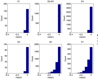
To obtain a better insight into the stability of the equi-librium states (Table 2), which we need to interpret some of the simulation results, we calculated the distribution of eigenvalues of the stable equilibrium points (Figure 2). For simplicity we report only the maximum eigenvalue of each equilibrium point that decides the stability and calcu-late the mean of the maximum eigenvalues across all simu-lations that reached the equilibrium point. The corner equilibria where either fixation or loss at a locus occurred (E6 and E7) have on average the lowest eigenvalues (E6, 20.033; E7, 20.043) and are therefore most stable. The eigenvalues in the edge equilibria where locus Aremains polymorphic (E4 and E5) are much higher (E4, 20.009; E5,20.0085) than those of E6 and E7, and the same is true for the symmetric equilibria (E1,20.01). The unsymmetric equilibria have the highest mean of the maximum eigenval-ues (E2 + E3, 20.00034). The unsymmetric equilibria are therefore the weakest of all stable equilibrium states. How-ever, we observe that the degree of stability is not related to the percentage of trajectories ending up in a state. For in-stance, we found about 2.5 times more trajectories converg-ing to unsymmetric equilibria compared to symmetric ones, which may be attributed to the fact that they are randomly distributed in the gamete space, whereas the symmetric ones are located on a line.
Selective sweeps occur at loci when a beneficial allele rises rapidly tofixation from a very low frequency. Fixation
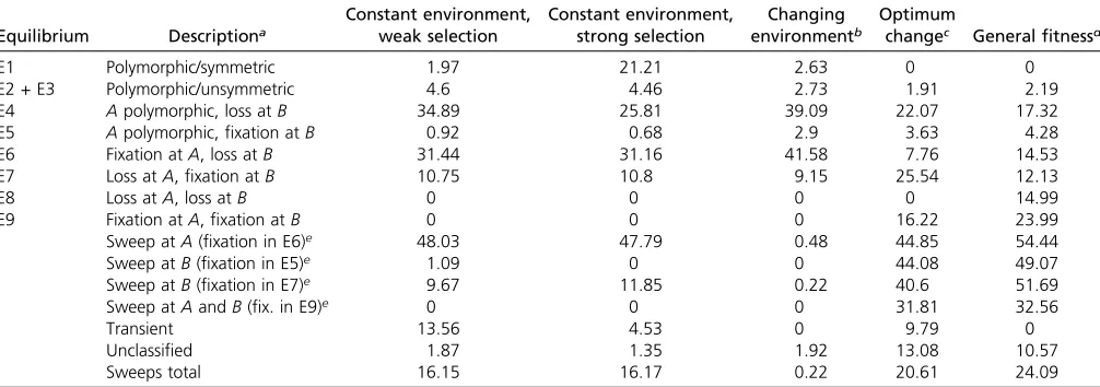
Table 2 Proportions (%) of trajectories that lead to one of the equilibria in the deterministic case
Equilibrium Descriptiona
Constant environment, weak selection
Constant environment, strong selection
Changing environmentb
Optimum
changec Generalfitnessd
E1 Polymorphic/symmetric 1.97 21.21 2.63 0 0
E2 + E3 Polymorphic/unsymmetric 4.6 4.46 2.73 1.91 2.19
E4 Apolymorphic, loss atB 34.89 25.81 39.09 22.07 17.32
E5 Apolymorphic,fixation atB 0.92 0.68 2.9 3.63 4.28
E6 Fixation atA, loss atB 31.44 31.16 41.58 7.76 14.53
E7 Loss atA,fixation atB 10.75 10.8 9.15 25.54 12.13
E8 Loss atA, loss atB 0 0 0 0 14.99
E9 Fixation atA,fixation atB 0 0 0 16.22 23.99
Sweep atA(fixation in E6)e 48.03 47.79 0.48 44.85 54.44
Sweep atB(fixation in E5)e 1.09 0 0 44.08 49.07
Sweep atB(fixation in E7)e 9.67 11.85 0.22 40.6 51.69
Sweep atAandB(fix. in E9)e 0 0 0 31.81 32.56
Transient 13.56 4.53 0 9.79 0
Unclassified 1.87 1.35 1.92 13.08 10.57
Sweeps total 16.15 16.17 0.22 20.61 24.09
aThe equilibria E1–E9 are defined following Bürger (2000, p. 205).
bEnvironmental changes were defined by random change of the original effects and selection coefficient. cIn the shifted optimum model (seeModels) the phenotypic optimum takes an arbitrary position 0,u,1. dIn the generalfitness model the effects have arbitrary values sampled from (0, 2) such thatAis major locus.
eSelective sweeps are defined here as trajectories that lead tofixation from very low initial frequencies (,0.01). Numbers denote the proportions offixations with initial
of alleles can be observed in corner equilibria at one of the loci (E6 and E7) or at both (E9). In Table 2 we report the proportion of trajectories that reached these equilibria from initially low frequencies (0.01). We observed that for 48% of the trajectories that were going tofixation atA(and loss at
B, E6) the initial allele frequency was ,0.01 at locus A. Hence, 48% of the fixations in E6 were classical sweeps (according to our definition). In contrast, only 11% of the 12% observedfixations atB(from E5 and E7) were selective sweeps. In total,16% of all trajectories that ended in one of the equilibria E1–E9 were selective sweeps. This propor-tion of sweeps is much higher than that observed by Pavlidis
et al. (2012) who found that 4% of the trajectories were sweeps when the initial conditions are randomly drawn from [0, 0.2]3[0, 1.0] and selection is strong (0.1#s#
1). Joint sweeps at both A and B do not occur in the de-terministic case under stabilizing selection, as this state is unstable. Selective sweeps occur exclusively for gA # 2gB
(as predicted in theModelssection).
Second, to better understand why the number of sweeps we observed is increased in comparison to Pavlidis et al.
(2012), we simulated the distribution of trajectories for strong selection (withssampled from [0.1,1]) and the same initial conditions as used above. We found that 10 times more trajectories converge to a polymorphic symmetric equi-librium (E1) because the double heterozygote is most fit. The proportions of sweeps at the edge equilibrium with A
polymorphic and fixation at B (E5, 0%), the corner with
fixation atAand loss atB(E6: 48%), and the other corner with loss atAandfixation atB(E7: 12%) remain about the same (16%). Hence, the difference from our result is largely attributable to the fact that in the standard neutral frequency
spectrum that we used here to determine the initial condi-tions, most initial frequencies are small.
We also estimated the mean time to equilibrium under weak selection. For the trajectories that lead to adaptive
fixations the mean time to equilibrium was 476 genera-tions, whereas for trajectories that lead to other equilibria (including the ones that remained transient) it was 1105 generations (P_ranksum = 2.8 3 10282). As depicted in Figure 3, for a large range of parameter values, we observe a relatively short mean time to equilibrium of200 gener-ations if recombination rate is sufficiently large (correspond-ing roughly to the range in which QLE holds; see Figure 1). Figure 3 also shows that the mean time to reach an equilib-rium (including fixation) gets longer for low values of the selection coefficient or the effect sizes. This means that for low values of these parameters the speed of fixation may become too small to cause sweeps. For the constant-environment model with strong selection we observe a mean time to equilibrium for trajectories that lead to adaptive
fixations of50 generations, whereas all other trajectories need60 generations (P_ranksum = 2.9310212). Hence, larger effects decrease on average the time to reach an equilibrium.
Third, we simulated a change in the environment for the symmetricfitness model as follows. We assume that a population has evolved first in a constant environment and reached one of the possible equilibria E1 to E7 in the proportions reported in Table 2 for the constant-environment model. From these proportions we then sample the ini-tial allele and gamete frequencies. Furthermore, we change randomly the effects and selection coefficient, thus
re-flecting an extreme case of an environmental change (see
below for biologically more realistic cases). Then we let the system converge to its new equilibrium points. More than 98% of the trajectories ended in one of the equilibria listed in Table 2. We observe that 42% of the trajectories are driven tofixation atAand loss atB(E6). Compared to the constant environment (with weak selection), we observe a slightly higher amount of trajectories that approached the edge equilibrium E4 (39%). The chance of detecting selective sweeps as fixation at locus A (E6, 42%) is very low (0.5%). At locus B the proportion of selective sweeps is 0.2%. Thus, the total number of sweeps is much lower than in the constant-environment model (0.2%). The reason is that in contrast to an initial condition under standard neutrality, the population is in this scenario preadapted be-fore the environmental change occurs;i.e., it sits in a state in which the allele frequencies are not clustered near the cor-ner (E8). However, soft sweeps may occur if the initial state is an edge equilibrium (e.g., E4).
Fourth, we simulated a change in the optimum according to Equation 18. In addition to the parameter values sampled according to Table 1, we sampled the new optimumufrom a uniform distribution of the interval (0, 1). The initial dition for the allele frequencies was chosen as for the con-stant-environment model (standard neutral allele frequency spectrum). Compared to the symmetricfitness model,.13% of the trajectories did not end up in one of the states E1–E9, suggesting that the equilibrium structure of this model is rather different from the symmetricfitness model (discussed further below). We found an increase of the proportion of trajectories (26%) that led to fixation at the minor locus and loss of the allele at the major locus (E7). Furthermore, in accordance with theory,fixations occur at both loci in 16% (E9) of the cases, in particular whenuis large. Indeed, in all
fixations the condition u$gAþ12gB was met (see remark
below Equation 20). Hence, selective sweeps are expected to be relatively frequent at both the major and the minor locus, as observed in 44% of the trajectories reaching the edge withfixation at locusB(E5, 4%), 45% of the trajectories that reach the corner E6 (8%), and 41% of the trajectories that reach the corner E7 (26%). From the simulations that go to
the corner withfixation at both loci (E9, 16%) 32% generate a selective sweep. Note that a sweep occurring at both loci has been counted as one sweep, as it is produced by merely one trajectory. In total,21% of all trajectories ending in E1–E9 led to selective sweeps atAorB, which is a slight increase relative to the symmetric fitness model (16%) and can be attributed to the change of the optimum. The amount of trajectories leading to an edge equilibrium with A polymor-phic and loss at B is much lower (22%) compared to the previously discussed models.
Fifth, we simulated the general fitness model and observed that 89% of the trajectories ended in one of the states E1–E9. We found an increase of simulations that led to corner equilibria compared to the symmetric fitness model. Convergence to extreme phenotypes is quite likely compared to the symmetricfitness model (loss atAandB, 15%; fixations at both A and B, 24%). Furthermore, the internal symmetric equilibrium is generally unstable (as pre-dicted in theModelssection). In total,24% of all trajecto-ries ending in E1–E9 led to selective sweeps atAorB. These results agree roughly with those of Pavlidiset al.(2012) and are expected because in the general fitness model the dou-ble heterozygote is not necessarily associated with the high-estfitness as in the symmetricfitness model.
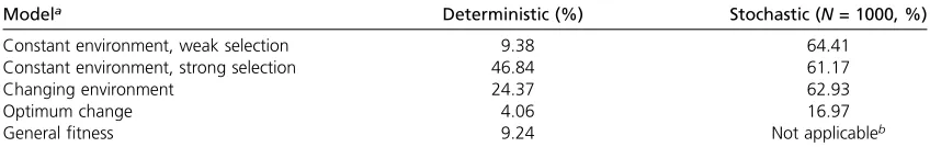
For all four models we also estimated the amount of LD between locusAandBusing the squared correlation coeffi -cientr2(Table 3). This coefficient that is defined only for the
internal polymorphic equilibria was measured at the end of each run. We note that the values in column 2 of Table 3 appear to be primarily determined by the symmetric equi-librium rather than the unsymmetric ones. Thus, for strong selection we found 47% LD relative to 9% for weak selec-tion, and LD is low if the polymorphic/symmetric equilib-rium (E1) does not exist as in the shifted optimum model. The reason is that LD is generally much stronger in the symmetric equilibrium. In our stochastic simulations (dis-cussed below) we observed generally higher LD, due to the action of drift.
Finally, we studied the probability of observing adaptive
fixations under biologically more realistic assumptions (see
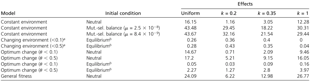
Table 4). The initial conditions were derived from a muta-tion–selection equilibrium (Orr and Betancourt 2001), with 0,s,0.1 and mutation rates of 8.431029per site per generation forDrosophila(Haag-Liautardet al.2007) and of 2.531028for humans (Nachman and Crowell 2000). The effects were sampled from a gamma distribution with the shape parameter k =0.2 and k =0.35, which have been previously measured for Drosophila and humans, respec-tively (Keightley and Eyre-Walker 2007). Furthermore,
k = 1 was chosen as an extreme case. We report the pro-portion of adaptivefixations observed from 10,000 simula-tions after 10,000 generasimula-tions for the various combinasimula-tions of models, initial conditions, and distributions of effect sizes (Table 4). Overall we observe that using the biologically more reasonable gamma-distributed effects, the proportion of selective sweeps is reduced in the constant-environment model (e.g., from 16 to 1% comparing the uniformly distrib-uted effects with gamma-distribdistrib-uted effects and k = 0.2). Similarly, in the general fitness model the percentage of
fixations is lower for gamma-distributed effects and realistic values of the shape parameter than for the effects sampled form the uniform distribution. In contrast, using the muta-tion–selection balance as initial condition strongly increases the chance of observing selective sweeps for the constant-environment model, as much more low-frequency variants are initially available that might go to fixation. For the changing-environment model, we also analyzed the impact of moderate environmental changes by altering the effects by 10 or 50%. In both cases the observed number of sweeps remains quite low, independent of the chosen effect size distribution. A more moderate optimum shift than in the original model reduced the proportion of sweeps to some extent compared to the results shown in Table 2.
We also tested the constant-environment model under the assumptions that the effects are derived from the initial frequencies using an exponential distributionaexp(2bp). We have chosen the parametera =0.5 andb =1 to match the distribution measured in Mackay et al. (2012). We observe a high proportion of trajectories going tofixation from initially low frequencies (30%). Hence, alleles with high effect sizes and initially low frequencies reachfixation quickly.
Stochastic simulations
We ran stochastic simulations in a similar way as described above to study the impact of genetic drift on the resulting
proportions of equilibria approached by the trajectories. Instead of ODEs, we used the system of corresponding difference equations (Willensdorfer and Bürger 2003). Gam-ete frequencies are sampled after each generation using the
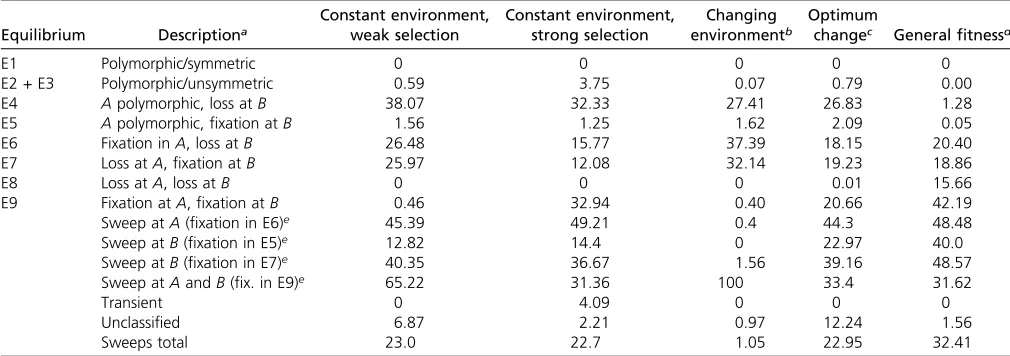
“mnrnd”function in Matlab (v. 6.1). As in the deterministic case we let the system evolve for 10,000 generations. Due to the random nature of genetic drift, equilibrium points can be approached, yet the trajectories may not stay at the deter-ministic equilibria. Therefore, we measured the proportion of trajectories that reside in aneinterval (withe=1023) of one of the respective equilibria after 10,000 generations (see Table 2 and Table 5).
For the constant-environment model and a population size ofN= 1000, the trajectories reside in the neighborhood of the unsymmetric polymorphic equilibria at low proportion (E2 + E3, 1%) compared to the edge equilibria (E4, 38%). This is not surprising given that their eigenvalues are closest to zero compared to the eigenvalues of the other equilibria. However, in the constant-environment model due to drift, losses atAandfixations atB(E7, 26%; see Table 5) occur more frequently than in the deterministic case (E7, 11%; see Table 2), and the same is true under the changing-environ-ment model. Consequently, sweeps at the minor locus are observed almost as often as at the major locus. This involves frequent crossings of the separatrices described above (for the QLE approximation). For example, assuming a constant environment and equal effects, the separatrices are defined as the diagonals in the pq plane. From 10,000 stochastic simulations with equal effects and a neutral allele frequency distribution as initial condition we observe 11% crossings of the separatrices. Selective sweeps at theBlocus are possible. Increasing the population size to .10,000 makes the rela-tive proportions of time spent in the equilibria similar to the percentages found in the deterministic case (data not shown).
Discussion
We have analyzed four versions of the two-locus model of stabilizing selection on a phenotypic trait to understand the signatures of selection at the molecular level. For symmetric
fitnesses we found for realistic parameter ranges (i.e., weak selection and loose linkage) essentially two evolutionary outcomes: fixation or polymorphism at the major locus (while the minor locus was monomorphic). At the genomic
Table 3 Average amount of linkage disequilibrium (r2) between the major and minor locus at the end of each run
Modela Deterministic (%) Stochastic (N= 1000, %)
Constant environment, weak selection 9.38 64.41
Constant environment, strong selection 46.84 61.17
Changing environment 24.37 62.93
Optimum change 4.06 16.97
Generalfitness 9.24 Not applicableb
level,fixations may be observed as classical selective sweeps if the initial frequency of the beneficial allele was very low and selection sufficiently strong or as sweeps from standing variation (soft sweeps). Polymorphic equilibria may be detected as allele frequency shifts. However, this is possible only if these events occurred relatively recently (Kim and Stephan 2000). In the following we discuss how the differ-ent versions of the model, the initial conditions of the ensu-ing evolutionary trajectories, and population size influence the relative abundance of these signatures.
Models
The symmetric viability model produces sweeps for16% of the trajectories if the initial frequencies were chosen accord-ing to the standard neutral site-frequency spectrum (Tajima 1989). This number is considerably higher than in the case of randomly drawn initial frequencies (Pavlidiset al.2012). The main reason is that most polymorphisms in the neutral frequency spectrum are singletons (i.e., occur once in a sam-ple) and are therefore centered around the state in which both loci are monomorphic (E8). The locus with the larger effects exhibits more selective sweeps than the locus with the minor effects. The amount of sweeps remains about the same for high-selection coefficients. However, more trajec-tories are found in the polymorphic equilibrium than for weak selection.
In the other two generalized models in which the trajectories started from initial frequencies sampled from the neutral frequency spectrum, the proportion of sweeps is even higher than that for the symmetricfitness model. For the model with an optimumu.0, we found that20% of the trajectories reach fixation starting from an initial fre-quency ,0.01, although the parameter values (other than
u) were drawn from the same distributions as for the sym-metricfitness model. This increase in the number of sweeps is due to the fact that a shift of the optimum to a positive value reflects directional selection on the phenotype. Under standard neutral initial conditions, the generalfitness model predicts that 24% of the trajectories lead to sweeps. The reason is that, as in the shifted optimum model, the double
heterozygote is not necessarily associated with the highest
fitness.
Initial conditions
The initial conditions of the trajectories studied in this article are usually drawn from the standard neutral site-frequency spectrum. This appears to be biologically more plausible than random initial frequencies. However, this difference of initial conditions may have a large influence on the ensuing trajectories. In other words, the evolutionary dynamics of the models are relatively sensitive to the basins of attraction of the underlying system. As we have empha-sized above, in the case of initial conditions following the standard neutral frequency spectrum, the number of sweeps is much higher than for random initial frequencies, as the initial frequencies are more centered around state in which both loci are monomorphic (E8). As expected, we found that the proportion of sweeps is even higher if the initial frequencies are drawn from a mutation–selection balance (Orr and Betancourt 2001), which show an excess of low-frequency alleles (Ohta 1973). The choice of the initial con-ditions appears to be more important for the symmetricfitness model, whereas the generalfitness model appears to be less sensitive to whether the initial frequencies are,0.0001 or 0.2 (see Pavlidis et al.2012, Figure 4).
On the other hand, assuming that a sudden environmen-tal shift occurs from an equilibrium state to which a pop-ulation has already been adapted, the number of sweeps observed may be drastically reduced. We observed this in our model of an environmental change in which we sampled the model parameters from the same distributions as for the other models. Many trajectories are driven from edges into a corner equilibrium. Thus, we found a very strong re-duction of classical sweeps and instead a large proportion of allele frequency shifts orfixations from standing variation.
Population size
All results discussed above were generated using the de-terministic version of the models. In our stochastic simu-lations, the effect of genetic drift due to a finite population
Table 4 Percentage of selective sweeps for various models, initial conditions, and distributions of effects
Effects
Model Initial condition Uniform k= 0.2 k= 0.35 k= 1
Constant environment Neutral 16.15 1.16 3.05 12.28
Constant environment Mut.-sel. balance (m= 2.531028) 43.48 29.45 18.22 30.31
Constant environment Mut.-sel. balance (m= 8.431029) 43.67 32.16 21.54 29.44
Changing environment (,0.1)a Equilibriumb 0.26 0.36 0.4 0
Changing environment (,0.5)a Equilibriumb 0.28 0.43 0.35 0.04
Optimum change (u,0.1) Neutral 14.67 0.71 2.09 9.46
Optimum change (u,0.5) Neutral 17.2 5.21 9.15 16.05
Optimum change (u,0.1) Equilibriumb 0.05 0.03 0.09 0.16
Optimum change (u,0.5) Equilibriumb 2.27 1.27 2.8 3.97
Generalfitness Neutral 24.09 6.22 12.98 26.77
aEffects were changed randomly relative to the initial effects by 10 or 50%.
size is twofold. First, the equilibrium points of the deter-ministic system, in particular, the less stable internal ones, are no longer attractive. As a consequence, more trajectories tend to approach the corner equilibria in which drift can no longer operate. Second, drift facilitates crossing of separa-trices, which is not possible in the deterministic system. For this reason, we occasionally observed for small population sizes (ofN= 1000) relatively large differences between the outcomes of the deterministic and stochastic simulations. For instance, in the changing-environment model, many more trajectories have approached the equilibrium E7 (loss atA,fixation atB) in the stochastic case than in the deter-ministic one. Similarly, we observe in all models a slightly higher proportion of sweeps in the stochastic case compared to the deterministic case. For larger population sizes (N.
10,000) the system approaches the deterministic version (data not shown).
Predictions of alternative models
We have quantified the frequency of selective fixations (leading to selective sweeps) in one of the most widely studied models of quantitative genetics, the two-locus model of stabilizing selection. In a similar analysis, this model has been extended from two to eight loci by Pavlidis et al.
(2012). Using the general fitness scheme, these authors found that the frequency of sweeps declines with the num-ber of loci. However, several classes of alternative models of stabilizing selection have been analyzed with respect to the maintenance of polygenic variation, for which we do not know to what extent they predict selectivefixations.
One of the simplest ways to maintain genetic variation in natural populations is to include mutation (Kimura 1965b; Turelli 1984; Barton 1986). In Barton’s model, selective
fixations have been detected after an optimum shift was
introduced. Although the frequency of sweeps was not esti-mated (de Vladar and Barton 2011, 2014), their simulations indicate that larger shifts of the optimum increase thefi xa-tion probability, as discussed above for the shifted optimum model. However, in none of the other mutation-stabilizing selection models was this issue addressed.
Polygenic variation could also be caused by pleiotropic effects of balanced polymorphisms (Turelli 1985; Barton 1990; Keightley and Hill 1990). An extension of Barton’s (1986) model including pleiotropy was proposed by Gimel-farb (1996). In this model, ndiallelic loci contribute addi-tively to n quantitative traits under stabilizing selection, such that each locus has a major effect on one trait and mi-nor effects on all other traits. It can be shown analytically that adaptivefixations are facilitated if the shift of the opti-mum of a trait after an environmental change is relatively large and the effects of the locus on the other traits small (unpublished results). Recently, pleiotropy was combined with mutation and stabilizing selection, and it was demon-strated that this is a sufficient mechanism to explain ob-served levels of genetic variation (Zhang and Hill 2002; 2005). In this class of models, real stabilizing selection works directly on the trait under study and apparent stabi-lizing selection is caused by the deleterious pleiotropic side effects of mutations on fitness. Therefore, these models are expected to predict extremely low fixation probabili-ties of new mutations, unless the degree of pleiotropy is much lower than generally thought (Wagner and Zhang 2011).
Acknowledgments
A.W. was supported by Volkswagen Foundation (ref. 86042). W.S. was supported from the German Research
Table 5 Proportions (%) of trajectories that lead to one of the equilibria in stochastic simulations (N= 1000) after 10,000 generations
Equilibrium Descriptiona
Constant environment, weak selection
Constant environment, strong selection
Changing environmentb
Optimum
changec Generalfitnessd
E1 Polymorphic/symmetric 0 0 0 0 0
E2 + E3 Polymorphic/unsymmetric 0.59 3.75 0.07 0.79 0.00
E4 Apolymorphic, loss atB 38.07 32.33 27.41 26.83 1.28
E5 Apolymorphic,fixation atB 1.56 1.25 1.62 2.09 0.05
E6 Fixation inA, loss atB 26.48 15.77 37.39 18.15 20.40
E7 Loss atA,fixation atB 25.97 12.08 32.14 19.23 18.86
E8 Loss atA, loss atB 0 0 0 0.01 15.66
E9 Fixation atA,fixation atB 0.46 32.94 0.40 20.66 42.19
Sweep atA(fixation in E6)e 45.39 49.21 0.4 44.3 48.48
Sweep atB(fixation in E5)e 12.82 14.4 0 22.97 40.0
Sweep atB(fixation in E7)e 40.35 36.67 1.56 39.16 48.57
Sweep atAandB(fix. in E9)e 65.22 31.36 100 33.4 31.62
Transient 0 4.09 0 0 0
Unclassified 6.87 2.21 0.97 12.24 1.56
Sweeps total 23.0 22.7 1.05 22.95 32.41
aThe equilibria E1 to E9 are defined following Bürger (2000, p. 205).
bEnvironmental changes were defined by random change of the original effects and selection coefficient. cIn the shifted optimum model (seeModels) the phenotypic optimum takes an arbitrary position 0,u,1. dIn the generalfitness model the effects have arbitrary values sampled from (0, 2) such thatAis major locus.
eSelective sweeps are defined here as trajectories that lead tofixation from very low initial frequencies (,0.01). Numbers denote the proportions offixations with initial
Foundation (Priority Program 1590, grant Ste 325/14-1). Part of this article was written at the Simons Institute for the Theory of Computing (University of California—Berkeley).
Literature Cited
Barton, N. H., 1986 The maintenance of polygenic variation through a balance between mutation and stabilizing selection. Genet. Res. 47: 209–216.
Barton, N. H., 1990 Pleiotropic models of quantitative variation. Genetics 124: 773–782.
Barton, N. H., 1998 The effect of hitch-hiking on neutral geneal-ogies. Genet. Res. 72: 123–133.
Barton, N. H., and P. D. Keightley, 2002 Understanding quantita-tive genetic variation. Nat. Rev. Genet. 3: 11–21.
Bürger, R., 2000 The Mathematical Theory of Selection, Recombi-nation,and Mutation. Wiley, New York.
Bürger, R., and A. Gimelfarb, 1999 Genetic variation maintained in multilocus models of additive quantitative traits under stabi-lizing selection. Genetics 152: 807–820.
Chevin, L. M., and F. Hospital, 2008 Selective sweep at a quanti-tative trait locus in the presence of background genetic varia-tion. Genetics 180: 1645–1660.
Crow, J., and M. Kimura, 1970 An Introduction to Population Ge-netics Theory. Burgess, Minneapolis.
de Vladar, H. P., and N. H. Barton, 2011 The statistical mechanics of a polygenic character under stabilizing selection, mutation and drift. J. R. Soc. Interface 8: 720–739.
de Vladar, H. P., and N. Barton, 2014 Stability and response of polygenic traits to stabilizing selection and mutation. Genetics 197: 749–767.
Endler, J., 1986 Natural Selection in the Wild. Princeton University Press, Princeton.
Falconer, D. S., and T. F. C. Mackay, 1996 Introduction to Quan-titative Genetics. Prentice Hall, London.
Fisher, R. A., 1930 The Genetical Theory of Natural Selection. Clar-endon Press, Oxford.
Gavrilets, S., and A. Hastings, 1993 Maintenance of genetic var-iability under strong stabilizing selection: a two-locus model. Genetics 134: 377–386.
Gimelfarb, A., 1996 Some additional results about polymor-phisms in models of an additive quantitative trait under stabi-lizing selection. J. Math. Biol. 35: 88–96.
Griffiths, R., and S. Tavaré, 1998 The age of a mutation in a gen-eral coalescent tree. Commun. Statist. Stoch. Models 14: 273– 295.
Haag-Liautard, C., M. Dorris, X. Maside, S. Macaskill, D. L. Halligan et al., 2007 Direct estimation of per nucleotide and genomic deleterious mutation rates in Drosophila. Nature 445: 82–85. Hermisson, J., and P. S. Pennings, 2005 Soft sweeps: molecular
population genetics of adaptation from standing genetic varia-tion. Genetics 169: 2335–2352.
Innan, H., and Y. Kim, 2004 Pattern of polymorphism after strong artificial selection in a domestication event. Proc. Natl. Acad. Sci. USA 101: 10667–10672.
Kaplan, N. L., R. R. Hudson, and C. H. Langley, 1989 The“ hitch-hiking effect”revisited. Genetics 123: 887–899.
Keightley, P. D., and A. Eyre-Walker, 2007 Joint inference of the distribution offitness effects of deleterious mutations and pop-ulation demography based on nucleotide polymorphism fre-quencies. Genetics 177: 2251–2261.
Keightley, P. D., and W. G. Hill, 1990 Variation maintained in quantitative traits with mutation-selection balance: pleiotropic side-effects onfitness traits. Proc. Biol. Sci. 242: 95–100.
Kim, Y., and W. Stephan, 2000 Joint effects of genetic hitchhiking and background selection on neutral variation. Genetics 155: 1415–1427.
Kim, Y., and W. Stephan, 2002 Detecting a local signature of genetic hitchhiking along a recombining chromosome. Genetics 160: 765–777.
Kimura, M., 1965a Attainment of quasi linkage equilibrium when gene frequencies are changing by natural selection. Genetics 52: 875–890.
Kimura, M., 1965b A stochastic model concerning the mainte-nance of genetic variability in quantitative characters. Proc. Natl. Acad. Sci. USA 54: 731–736.
Lande, R., 1983 The maintainance of genetic variability by muta-tion in a polygenic character with linked loci. Genet. Res. 26: 221–235.
Lynch, M., and B. Walsh, 1998 Genetic Analysis of Quantitative Traits. Sinauer Associates, Sunderland, MA.
Mackay, T. F., S. Richards, E. A. Stone, A. Barbadilla, J. F. Ayroles et al., 2012 The Drosophila melanogaster genetic reference panel. Nature 482: 173–178.
Maynard Smith, J., and J. Haigh, 1974 The hitch-hiking effect of a favourable gene. Genet. Res. 23: 23–35.
Nachman, M. W., and S. L. Crowell, 2000 Estimate of the muta-tion rate per nucleotide in humans. Genetics 156: 297–304. Nielsen, R., S. Williamson, Y. Kim, M. J. Hubisz, A. G. Clarket al.,
2005 Genomic scans for selective sweeps using SNP data. Ge-nome Res. 15: 1566–1575.
Ohta, T., 1973 Slightly deleterious mutant substitutions in evolu-tion. Nature 246: 96–98.
Orr, H. A., 2005 The genetic theory of adaptation: a brief history. Nat. Rev. Genet. 6: 119–127.
Orr, H. A., and A. J. Betancourt, 2001 Haldane’s sieve and adap-tation from the standing genetic variation. Genetics 157: 875– 884.
Pavlidis, P., J. D. Jensen, and W. Stephan, 2010 Searching for footprints of positive selection in whole-genome SNP data from nonequilibrium populations. Genetics 185: 907–922.
Pavlidis, P., D. Metzler, and W. Stephan, 2012 Selective sweeps in multilocus models of quantitative traits. Genetics 192: 225–239. Pritchard, J. K., and A. Di Rienzo, 2010 Adaptation: not by sweeps
alone. Nat. Rev. Genet. 11: 665–667.
Pritchard, J. K., J. K. Pickrell, and G. Coop, 2010 The genetics of human adaptation: hard sweeps, soft sweeps, and polygenic adaptation. Curr. Biol. 20: R208–R215.
Robertson, A., 1956 The effect of selection against extreme devi-ants based on deviation or on homozygosis. J. Genet. 54: 236– 248.
Stephan, W., 1995 An improved method for estimating the rate of
fixation of favorable mutations based on DNA polymorphism data. Mol. Biol. Evol. 12: 959–962.
Stephan, W., 2010 Genetic hitchhikingvs.background selection: the controversy and its implications. Philos. Trans. R. Soc. Lond. B Biol. Sci. 365: 1245–1253.
Stephan, W., T. H. E. Wiehe, and M. W. Lenz, 1992 The effect of strongly selected substitutions on neutral polymorphism: ana-lytical results based on diffusion theory. Theor. Popul. Biol. 41: 237–254.
Tajima, F., 1989 Statistical method for testing the neutral muta-tion hypothesis by DNA polymorphism. Genetics 123: 585–595. Turchin, M. C., C. W. Chiang, C. D. Palmer, S. Sankararaman, D. Reichet al., 2012 Evidence of widespread selection on stand-ing variation in Europe at height-associated SNPs. Nat. Genet. 44: 1015–1019.
Turelli, M., 1985 Effects of pleiotropy on predictions concerning mutation-selection balance for polygenic traits. Genetics 111: 165–195.
Wagner, G. P., and J. Zhang, 2011 The pleiotropic structure of the genotype-phenotype map: the evolvability of complex organ-isms. Nat. Rev. Genet. 12: 204–213.
Willensdorfer, M., and R. Bürger, 2003 The two-locus model of Gaussian stabilizing selection. Theor. Popul. Biol. 64: 101– 117.
Zhang, X. S., and W. G. Hill, 2002 Joint effects of pleiotropic selection and stabilizing selection on the maintenance of quantitative genetic variation at mutation-selection balance. Genetics 162: 459–471. Zhang, X. S., and W. G. Hill, 2005 Evolution of the environmental
component of the phenotypic variance: stabilizing selection in changing environments and the cost of homogeneity. Evolution 59: 1237–1244.