Influence of Gene Interaction on Complex Trait Variation with Multilocus Models

HIGHLIGHTED ARTICLE INVESTIGATION

In

fl

uence of Gene Interaction on Complex Trait

Variation with Multilocus Models

Asko Mäki-Tanila*,1_{and William G. Hill}†

*Biotechnology and Food Research, MTT Agrifood Research Finland, 31600 Jokioinen, Finland, and†Institute of Evolutionary

Biology, School of Biological Sciences, University of Edinburgh, Edinburgh EH9 3JT, United Kingdom

ABSTRACTAlthough research effort is being expended into determining the importance of epistasis and epistatic variance for complex traits, there is considerable controversy about their importance. Here we undertake an analysis for quantitative traits utilizing a range of multilocus quantitative genetic models and gene frequency distributions, focusing on the potential magnitude of the epistatic variance. All the epistatic terms involving a particular locus appear in its average effect, with the number of two-locus interaction terms increasing in proportion to the square of the number of loci and that of third order as the cube and so on. Hence multilocus epistasis makes substantial contributions to the additive variance and does not,per se, lead to large increases in the nonadditive part of the genotypic variance. Even though this proportion can be high where epistasis is antagonistic to direct effects, it reduces with multiple loci. As the magnitude of the epistatic variance depends critically on the heterozygosity, for models where frequencies are widely dispersed, such as for selectively neutral mutations, contributions of epistatic variance are always small. Epistasis may be important in understanding the genetic archi-tecture, for example, of function or human disease, but that does not imply that loci exhibiting it will contribute much genetic variance. Overall we conclude that theoretical predictions and experimental observations of low amounts of epistatic variance in outbred pop-ulations are concordant. It is not a likely source of missing heritability, for example, or major influence on predictions of rates of evolution.

E

PISTATIC variance in quantitative traits arises from the interaction effects or epistasis between segregating genes at two or more loci that affect these complex traits. Such gene interaction is a common phenomenon because many factors have, for example, a regulatory role in a hierarchical system (Phillips 2008). The statistical theory of quantitative genetics following Fisher (1918) is based on a partition between av-erage effects across loci, which contribute to the additive genetic variance, and to interactions within loci and between loci, which contribute to the dominance and epistatic vari-ance, respectively (Cockerham 1954; Kempthorne 1954). The magnitudes of these components of the genotypic variance each depend on the frequencies, the effects, and the interac-tions among the contributing genes (see also Falconer and Mackay 1996; Lynch and Walsh 1998). The actual causal genetic factors are usually not known, but many quantitative

genetic analyses, including selection on metric traits, have been applied successfully without such knowledge.

Among quantitative geneticists, interest in epistasis con-tinues, both to understand the genetic architecture and as a potential way to improve the genomic predictions of disease and quantitative traits, utilizing some of the unexplained parts of the genetic variation (e.g., Carlborg and Haley 2004; Nelson

et al.2013; Mackay 2014). Despite the obvious interactions in the biological system, it has, however, been argued that the proportion of the genotypic variance contributed by epistatic variance expected in outbred populations is small and that data generally support this prediction (Hillet al.2008). The theory is based mainly on population and statistical genetics argu-ments (the data of a more indirect form): for many traits the covariances among relatives could largely be explained by ad-ditive models, albeit estimation of epistatic varianceper sewith much precision is difficult in most outbred population struc-tures. Hemaniet al.(2013) in contrast, taking an evolutionary perspective, have argued that much of the variation that will remain segregating long term in populations under natural section will be epistatic. It is notable, however, that the loci in the models they simulated that were still segregating all Copyright © 2014 by the Genetics Society of America

doi: 10.1534/genetics.114.165282

Manuscript received April 14, 2014; accepted for publication June 19, 2014; published Early Online July 1, 2014.

showed overdominance, for which direct data are limited (e.g., Charlesworth and Charlesworth 2009). Using models with mul-tiple loci and two-locus interactions in populations evolving with bottlenecks, Ávilaet al.(2014) found only small contributions of epistatic variance. Further, it has been argued that the magni-tude of epistatic variation is essentially irrelevant in evolution (and in animal breeding) (Crow 2010), because rates of evolu-tionary change depend only on the additive variance, even in epistatic and tightly linked systems (Kimura 1965; Nagylaki 1993). Nevertheless Nelsonet al.(2013) have recently argued that epistasis has been ignored in quantitative genetics and in its evolutionary studies because of convenience, and consequently statements about its insignificance are misleading.

Genomics offers tools that go much deeper, to identify the genes involved and their interactions within the system, perhaps thereby providing an understanding of the causes of specific complex diseases or traits and a route to their im-provement. There has, therefore, been a surge of interest in estimating the magnitude of epistasis and understanding its source. Despite the challenges in estimation, thousands of QTL have been found and manyfindings of interaction effects reported in crosses of divergent lines of chicken (Pettersson

et al.2011), yeast (Bloomet al.2013), andDrosophila(Huang

et al.2012). Further, there is recent evidence of detection of epistatic loci for levels of gene expression in human popula-tions (Hemaniet al.2014; Brownet al.2014).

Nevertheless the variation contributed by these epistatic loci detected in segregating populations is generally found to be small (Huanget al.2012; Brownet al.2014; Hemaniet al.

2014), whichfits with the theoretical predictions (Hillet al.

2008) that only at high heterozygosity levels do loci contrib-ute much epistatic variance; Bloomet al.(2013) note that the epistatic variance they found would have been much lower had they not been using an F1-based population.

The genetic variation accounted for by significant SNPs in genome-wide association studies (GWAS) in humans for both metric traits such as height and for multifactorial disease traits has typically been substantially less than the estimates of the additive genetic variation found in conventional pedigree-based quantitative genetic analyses. For example, the top 150 loci identified by SNPs account for only 10% of the variance in human height (Lango-Allen et al.2010). If all SNPs arefitted without constraint as to statistical significance, the amount explained rises to40% (Yanget al.2011) but still falls well short of the estimates of80% based on cova-riances among relatives. Several hypotheses for the so-called

“missing heritability” (Manolio et al. 2009) have been put forward, among these that epistasis is inflating the pedigree-based estimates (Zuket al.2012).

We therefore have some dichotomy between, on the one hand, those who argue that, although there may be epistasis, the epistatic variance contributed is likely to be small and generally we can ignore its contribution because it is unimportant, and on the other those who argue that this is a blinkered view. We cannot resolve this here, but we do attempt to provide a stronger theoretical base to the arguments. The analysis and inferences of

Hill et al. (2008) took into account the size and direction of interaction effects and the allele frequencies or heterozygosity at all contributing loci. Models were, however, based on pairs of loci, yet as quantitative geneticists have long assumed, have subsequently inferred from the continuing responses to selection for many traits in experiments and breeding programs, and now inferred more directly from GWAS, very many loci influence each trait. For multiple loci (n), however, the numbers of pairs with potential two-way interaction among loci increases as n2 [strictly 1/2n(n–1)], three-way interactions asn3_{, etc., and so it} is possible that merely accounting for interactions among pairs of loci gives a biased impression.

In this article we therefore consider the magnitude of epistatic variance expected in outbred populations for multilocus models to check on the robustness of the argument that most variance is likely to be additive genetic. We concentrate initially on models without dominance or interactions involving domi-nance, partly for simplicity of exposition and partly because we showed previously that additive variance is also expected to contribute much more than the dominance variance (Hillet al.

2008). We consider alternative distributions of the gene fre-quency within the populations at segregating loci affecting the trait because these have an important impact on the magnitude of the genotypic variance and its components. As these distribu-tions are not static in populadistribu-tions evolving under selection, we also consider the impact of consequent gene frequency changes.

Analysis

Genetic model with no dominance

We assume that there arenloci, each of which has two alleles Aior ai,i= 1,. . .,n, with frequenciespiand 1–pi,

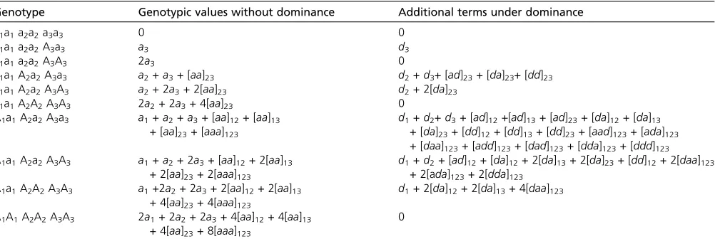
respec-tively. We further assume that there is Hardy–Weinberg and linkage equilibrium among all loci. Genotypic values are given in Table 1 (second column) for examples of alternative genotypes, and those for other genotypes are analogous,e.g., that for A1A1a2a2A3a3is 2a1+a3+ 2[aa]13(cf. fourth row). The model readily extends to more loci and to dominance (see below and third column of Table 1) and is fully parameterized.

The population mean without dominance is

m¼2X

i

piaiþ4

X

i

X

j.i pipj½aaij

þ8X

i

X

j.i

X

k.j.ipipjpk½aaaijkþ. . .:

With H–W and linkage equilibrium, average effects (also called

For locusi, the average effect including up to third-order interaction terms is

ai¼

1 2

@m

@pi

¼aiþ2

X

j6¼i

pj½aaijþ4

X

j6¼i

X

k6¼i;k.jpjpk½aaaijk þ. . .; i¼1; :::;n:

(1)

The additive variance is obtained by summing over thenloci

VA¼

X

i

2pið12piÞ

1 2@m=@pi

2

¼X

i Hia2i;

whereHi= 2pi(1–pi) is the heterozygosity at locusi.

Sim-ilarly additive 3 additive interaction effects and variances are

ðaaÞij¼

1 4

@2

m

@pi@pj

¼ ½aaijþ2

X

k6¼i;j

pk½aaaijk

þ4 X

l;k6¼i;j;l.k

pkpl½aaaaijklþ. . .; 1#i,j#n;

(2)

VAA¼

X

i

X

j.iHiHjðaaÞ 2 ij;

ðaaaÞijk¼

1 8

@3_m @pi@pj@pj

¼ ½aaa_ijkþ2 X

l6¼i;j;k

pl½aaaaijkl

þ. . .; 1#i,j,k#n;

VAAA¼

X

i

X

j.i

X

k.jHiHjHkðaaaÞ 2 ijk;

and so on, with the nth such partial derivatives giving n -locus epistatic effects and variances.

For three loci, for example,

a1¼a1þ2p2½aa12þ2p3½aa13þ4p2p3½aaa123;

ðaaÞ12¼ ½aa12þ2p3½aaa123 and ½aaa123¼ ½aaa123;

and therefore

VA¼

X

i Hi

a2_i þ4pjai½aaijþ4pkai½aaikþ4p2j½aa 2 ij

þ4p2_k½aa_ik2 þ8pjpk½aaij½aaikþ8pjpkai½aaaijk þ16p2_jpk½aaij½aaaijkþ16pjp2k½aaik½aaaijk þ16 p2_jp2_k½aaa2_ijk

;  where i6¼j6¼k;

(3a)

VAA¼

X

i

X

j.iHiHj

½aa2ijþ4pk½aaij½aaaijk

þ4p2_k½aaa2_ijk

  for k6¼i;j; (3b)

VAAA¼H1H2H3½aaa2123: (3c)

The key to subsequent results is that, because two- and three-locus interactions enter the average effects and additive variance, they can make a major contribution toVA, depend-ing on their allele frequencies and sign. Similarlyk-locus in-teraction effects contribute to the epistatic variances of order

,k, whereas single-locus contributions and interaction effects of order lower thankdo not.

Numbers and magnitude of terms in variance components

While it is assumed that many loci determine most quanti-tative traits, the number (n) is not known. To obtain some understanding of how the relative magnitudes of additive and Table 1 Genotypic values for representative genotypic combinations for a three-locus diploid model including two- and three-locus interaction effects

Genotype Genotypic values without dominance Additional terms under dominance

a1a1a2a2a3a3 0 0

a1a1a2a2A3a3 a3 d3

a1a1a2a2A3A3 2a3 0

a1a1A2a2A3a3 a2+a3+ [aa]23 d2+d3+ [ad]23+ [da]23+ [dd]23

a1a1A2a2A3A3 a2+ 2a3+ 2[aa]23 d2+ 2[da]23

a1a1A2A2A3A3 2a2+ 2a3+ 4[aa]23 0

A1a1A2a2A3a3 a1+a2+a3+ [aa]12+ [aa]13 + [aa]23+ [aaa]123

d1+d2+d3+ [ad]12+[ad]13+ [ad]23+ [da]12+ [da]13 + [da]23+ [dd]12+ [dd]13+ [dd]23+ [aad]123+ [ada]123 + [daa]123+ [add]123+ [dad]123+ [dda]123+ [ddd]123 A1a1A2a2A3A3 a1+a2+ 2a3+ [aa]12+ 2[aa]13

+ 2[aa]23+ 2[aaa]123

d1+d2+ [ad]12+ [da]12+ 2[da]13+ 2[da]23+ [dd]12+ 2[daa]123 + 2[ada]123+ 2[dda]123

A1a1A2A2A3A3 a1+2a2+ 2a3+ 2[aa]12+ 2[aa]13 + 4[aa]23+ 4[aaa]123

d1+ 2[da]12+ 2[da]13+ 4[daa]123

A1A1A2A2A3A3 2a1+ 2a2+ 2a3+ 4[aa]12+ 4[aa]13 + 4[aa]23+ 8[aaa]123

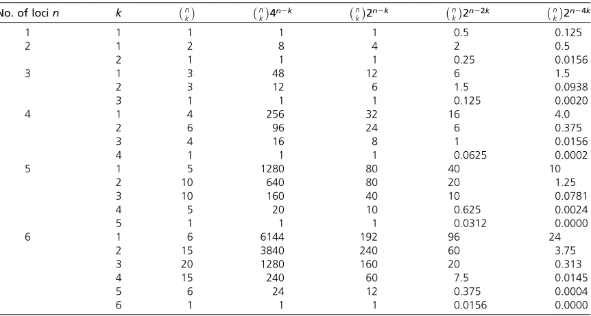
epistatic variance depend on n, we undertake some simple calculations on the basis that the partition will depend at least to some extent on the numbers of terms contributing to each. For the additive variance there are contributions fromnloci, and expansions such as in Equations 1 and 3a show that for each locus there are

1 þ

n21 1

þ

n21 2

:::þ1 ¼ 2n21

terms in the expression for the average effects and thus

n22(n21)_=n4n21_{in all when effects are squared (counting} terms such asai[aa]jkand [aa]jkaiseparately). There are more

pairs, trios etc. of loci contributing epistatic variance, but the numbers of terms they each comprise are reduced. For VAA there aren_k = 1/2n(n2 1) pairs of loci but 4n2 2_terms in each pair when squared (Equation 3b). In general, there are a total ofn_k4n2k_{terms for thekth-order epistatic variance}

among n loci. While terms such as [aa][aaa] that comprise products of different interaction effects may be negative, _n

k

2n2k_{are squared terms and therefore nonnegative.}

In the formulae for the average and other effects, terms inL

loci have a coefficient of 2L2k 21_{,e.g., 4 for p}

jpk[aaa]ijkin

Equation 1. But coefficients involving products of gene fre-quencies also appear in these same terms, each of which take values of 0.5 when gene frequencies are one-half. Thus if we assume gene frequencies are 0.5, which is when epistatic var-iance is typically at a maximum, this cancels the coefficients of 2 alluded to above. Hence while there are arguments for in-cluding other terms in these simple models, as a basis we re-strict them just to assuming these factors of two cancel. Hence the sum of weighted terms isn

k

4n2k_{and of squared terms is}

_n

k

2n 2 k_{. Examples of these figures are given in Table 2,}

which shows how the number of contributions to the varian-ces, particularly the additive variance, can be large indeed.

Heterozygosity has a maximum of 0.5 atP= 0.5, when, in the absence of epistasis, the additive variance is then at a max-imum. As the epistatic variances among k loci depend on products of k heterozygosity terms, the epistatic variances are likely to contribute correspondingly less to the genotypic varianceVGthan doesVA, and most of the epistatic variance is likely to derive from second-order components. Thus if we include heterozygosity in the calculations, letting H be an

“average”or representativefigure, thekth component of var-iance is of orderHkn

k

4n2k_{. IfH= 0.5, its maximum, the}

weighted number of terms, becomes (1/2)kn k

2n 2 k ₌

_n

k

4n2k_{, of which}n k

2n22k_{are squared terms. Further,}

in all but populations derived from F1 crosses, mean heterozy-gosity will be less than one-half, and we subsequently consider the impact of different allele frequency distributions on the ex-pected proportion of epistatic variance. Accordingly, the weighted numbers of terms becomen

k

4n24k_andn k

2n24k_,

re-spectively,i.e., very much smaller indeed askincreases. Examples of the computed values are given in Table 2. These calculations for multiple loci are intended to serve only as a guide, but illustrate why a high proportion of epistatic

variance is unlikely, because even very strong multilocus gene–gene interactions do not automatically lead to a high proportion of epistatic components in the genetic variation (cf. Cheverud and Routman 1995).

Examples

The relative magnitude of additive and epistatic variances for two tofive loci including all possible gene–gene interactions is summarized in Figure 1 for two models with the frequency of the increasing allele the same at all loci. In both, the magnitude of gene and (absolute value of) interaction effects are also assumed to be the same at all loci, and are either all synergistic ([aa] = [aaa] =. . .=a) or antagonistic ([aa] = [aaa] =. . .=

2a). As expected from the above arguments, the genetic var-iance in many of these examples is seen to be mainly additive and the remainder mainly additive3additive, such that higher-order epistatic variances can generally be ignored. Gene inter-actions generally make the most substantial contributions toVA when the frequency of the increasing allele is very low, and only negative (antagonistic) interactions cause relatively large ratios of epistatic to additive variance because terms such asai[aa]jkin VAare then negative.

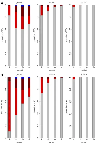
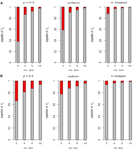
Expected variances for different allele frequency distributions

The components of genetic variance and their relative magnitudes depend on the allele frequencies in addition to the individual gene effects and their interactions. Although there is little information on allele frequencies for quantitative trait genes, it is possible to predict their frequency distribution under different assumptions about relevant evolutionary factors, such as mutation, selection, finite population size (drift), and migration. Allele frequencies of 0.5,i.e., from a re-cent inbred cross, serve as one reference point and, as evi-dence suggests that many genes influence metric traits and so there is presumably very mild natural selection on them, the-ory for neutral alleles infinite populations serves as another. Two allele frequency distributions are considered, each with mean 0.5. One is a closedfinite population under drift without mutation, when the steady-state distribution is uniform over (0, 1) (e.g., Crow and Kimura 1970; Falconer and Mackay 1996). The other is for mutation–drift balance, when the frequency density of mutants is proportional to 1/p(Wright 1931); but, if increasing and decreasing mutants for the trait are assumed equally likely, the frequency distribution of segregating increasing mutants for the trait is U shaped, withf(p)}1/[p(1–p)] (Hillet al.2008). The distributions and expected heterozygositiesE(H) are

F2 based population : p¼0:5; EðHÞ ¼0:5

uniform : fðpÞ ¼1;0#p#1;EðpÞ ¼0:5;EðHÞ ¼0:333

U shaped : fðpÞ}1=½pð12pÞ;1=ð2NÞ#p#11=ð2NÞ;

 EðpÞ ¼0:5;EðHÞ 1=½2lnð2NÞ:

For the U-shaped distribution and effective population sizes

0.0944, 0.0658, and 0.0410, respectively. Examples are given in Figure 2 for the partition of variance under different epistatic and frequency distribution models for three and more loci. The largest proportion of epistatic variance is expected when P= 0.5 while uniform and U-shaped allele frequency distributions yield mostly additive variance, even with antagonistic gene–gene interaction. In all cases the epistatic variance is almost entirely contributed by the two-locus epistatic variance.

Whennloci contribute nearly equally to the variation, for given total genetic variance, their individual effects a will tend to decline approximately in proportion to 1=pffiffiffin as n

increases to and, similarly, epistatic interactions between pairs of loci [aa] are likely to decline roughly in proportion to 1/nand between trios of loci [aaa] by 1=ðnpffiffiffinÞ. The dimin-ishing relative size of the interaction effects with increasing number of loci shown above for those with equal effect is therefore exacerbated as the interaction terms become indi-vidually smaller (Figure 2Avs.Figure 2B). Hence, if there is a very large number of interacting loci (say.50) almost all the variation is expected to be additive. If their effects differ greatly, then the results become like those for fewer loci.

To illustrate the effect of increasing the number of loci, we include interactions only up to second or third order with positive (or negative) sign consistent over loci. Again, unless interaction terms are such that, for example, [aa] is negative and its products in the expressions for variance balance the positivea2_{and [aa]}2_{term (Figure 2), the general conclusion} is that, with a very large number of loci, only in special cases are the positive and negative terms likely to counter each other and the epistatic variance to be larger than the addi-tive variance. Similarly, as the number of loci become very

large, epistatic variance of higher order also become trivial compared toVAA.

Dominance

The diploid models can easily be extended to incorporate dominance effects and Kojima’s (1959) method can be used to compute the different components of genetic variance. This has been done to illustrate the close correspondence with ad-ditive models (Appendix 1). The inclusion of dominance intro-duces three additional two-locus interaction terms [ad], [da], and [dd]. Similar to the way in which the additive interactions contribute to the additive variance, the dominance interactions contribute to both the additive and dominance variance. The number of additional terms in the formulae for the variances increases rapidly, so for clarity, results are given only for two loci with positive interactions (Figure 3).

As in the case of additive interactions, the proportion of epistatic variance is small, in particular when allele frequen-cies are not concentrated at intermediate values. The pro-portion of dominance variance stays the same or is slightly increased when adding the dominance interaction while the ratio between additive and dominance variance is not changed, implying that the interaction terms contribute to these variances in the same way. When the allele frequencies are 0.5 there is most epistatic variance, but its contribution rapidly decreases for a higher number of loci, with the same pattern as with only additive effects and interactions. Effect of selection on the expected variances

For traits under stabilizing selection with intermediate opti-mum, frequencies of increasing and decreasing alleles will also tend to be distributed around 0.5 as in the neutral case. In a

Table 2 Number of variance components of orderkamongnlocin_k(k= 1 denotes additive variance), numbers of

terms in the expansion of the variance from effects, and number of such terms that are squared terms,n_k2n2k

No. of locin k n_k n_k4n2k _kn2n2k _kn2n22k n

k

2n24k

1 1 1 1 1 0.5 0.125

2 1 2 8 4 2 0.5

2 1 1 1 0.25 0.0156

3 1 3 48 12 6 1.5

2 3 12 6 1.5 0.0938

3 1 1 1 0.125 0.0020

4 1 4 256 32 16 4.0

2 6 96 24 6 0.375

3 4 16 8 1 0.0156

4 1 1 1 0.0625 0.0002

5 1 5 1280 80 40 10

2 10 640 80 20 1.25

3 10 160 40 10 0.0781

4 5 20 10 0.625 0.0024

5 1 1 1 0.0312 0.0000

6 1 6 6144 192 96 24

2 15 3840 240 60 3.75

3 20 1280 160 20 0.313

4 15 240 60 7.5 0.0145

5 6 24 12 0.375 0.0004

6 1 1 1 0.0156 0.0000

The number of squared terms are also shown multiplied by the maximum heterozygosity (1/2)k_{for thekorder term,i.e.,}n k

2n22k_{, and also by}

a more typical mean heterozygosity in a long standing population (1/8)k,i.e.,n k

population newly under directional selection, the mean fre-quency of increasing alleles will increase.0.5, but under long continued selection stabilize as new mutants come in. Hence we consider the results for neutral distributions to be still relevant. We examine some limited examples, however.

In a population under selection the contribution of epistatic to total variance changes as frequencies change. Thus as Hansen (2013), for example, emphasizes, although selection response at any given time depends almost entirely on the additive variance (Kimura 1965; Crow 2010), the long-term trajectory depends on the nature of the interactions among

the loci. Further, allele frequency distributions can no longer remain symmetric aroundP= 0.5 under directional selection. In a small investigation of the robustness of some of our con-clusions under selection, for example, that a high proportion of VG is contributed by VA, we used transition probability matrices to obtain the distributions for pairs of unlinked loci, modeling with quite small population size values. For sim-plicity a haploid model with population sizeNhwas assumed. Details of the model are given inAppendix 2.

Several simple situations were modeled using two loci with synergistic or antagonistic epistatic effects ([aa] = +a

or–a). These included cases where (i) the increasing alleles at each locus were mutants at initial frequency 1/Nh, (ii) the frequency at one locus was at steady state under neutrality (i.e., U shaped) and at the other locus a mutant allele of either increasing or decreasing effect, and (iii) initial fre-quencies at the two loci were set as either 1/Nh or 1–1/

Nh with equal probability. Components of variance were obtained by averaging over 100 generations.

Detailedfindings are given inAppendix 2. Although lim-ited in scope, the results are clear: the asymmetry in the allele frequency distributions caused by selection does not

seem to influence the relative proportions of additive and nonadditive variance and thus substantially alter the gen-eral expectation that the proportion of epistatic variance is likely to be small.

Discussion

Mainfindings

When the genetic variation is caused by segregation at many loci, the magnitude of the epistatic variance is almost certain to be trivial relative to the additive variance. This result is

Figure 2 Expected components of genetic variance under gene–gene interaction. As Figure 1, but for fewer loci, assumed allele frequency (p)

distributions ofP= 0.5, uniform and U-shaped (N= 100) distribution (respective expected heterozygosities E(H)) with two- and three-locus interaction

effects with (A) constant or (B) declining gene and negative interaction effects with increasing number of loci. (A) [aaa] = [aa] = 2a. (B)

nearly invariant to the order of the interaction, allele fre-quencies, and type and magnitude of interaction effects. The models show how the gene-interaction effects appear in the average effects and contribute to the additive variance and produce more positive terms there than in the epistatic components. The epistatic components depend on the magni-tude of heterozygosity and are generally small for low hetero-zygosity. For the same reasons, under most of the assumptions the majority of the epistatic variance is due to the two-locus epistatic component.

When the variation is due to only a few interacting loci or there are major genes with substantial gene–gene interac-tion effects segregating in the populainterac-tion, there are no gen-eral patterns in the proportion of epistatic variance, but the following are the main observations: high heterozygosity (or allele frequency 0.5) and/or negative interaction can gener-ate high proportions of epistatic variance; the proportion of the variance that is epistatic variance is lowest at low het-erozygosity, notably for the U-shaped allele frequency distri-bution but even for the uniform distridistri-bution compared to

P= 0.5; and deviations from symmetry of the distribution caused by mild selection do not increase the low proportion of epistatic variance.

Models and assumptions

Only biallelic loci were analyzed but we cannot see that the general results would be fundamentally affected if loci are multiallelic. Each of themtwo-way interactions formalleles at each locus with no dominance appear in the average effects for themalleles atthemloci, givingm3_{terms after} squaring effects, whereas the number of additive3additive effects and variance components increases only in propor-tion to the number of allelic pairs,m2_{, as each has only one}

two-way interaction. Although we focused on models with-out dominance, as the interaction effects containing domi-nance contribute to the domidomi-nance variance in the same way as do the additive3additive effects to the additive variance, the qualitative finding remains that the proportion of epi-static variance in the total genotypic variance is small.

Epistasis also arises, even with infinitesimal additive effects on some underlying variable, if there is a nonlinear relation-ship between genotypic and observed phenotypic values, such as with a multiplicative, optimum, or threshold model (e.g., Wright 1931; Dempster and Lerner 1950; Cockerham 1959). Kojima’s (1959, 1961) methodology provides a simple way to partition the genotypic variance and can also be applied to these models. Basically, the proportion of epistatic variance is high only when the transformation departs far from linearity: a high coefficient of variation in the multiplicative model, the population mean near the optimum value in the optimum model, and with a proportion truncated near 0 or 1 in the threshold model (see also Mäki-Tanila and Hill 2014).

In an attempt to explain some of the missing heritability, especially that estimated from human twin studies, Zuk

et al. (2012) suggested that the additive component was overestimated, biasedinter aliaby epistatic variance. They proposed an extreme type of threshold model, with the all-or-none output dependent on whether, in some underlying system of multiple identically independently (i.i.d.) nor-mally distributed variables, the lowest exceeded the cutoff. This model undoubtedly generates substantial epistatic var-iance, but has been queried both because it is sensitive to assumptions, such as i.i.d. and is biologically implausible (Stringeret al.2013). Indeed there is little evidence of such limiting pathways, and models based on flux through sys-tems without “limiting steps” have firmer foundation (Kacser and Burns 1973). Analysis of genetic models offlux in pathways shows that largely additive variance is to be expected (Keightley 1989; Hill et al. 2008). Much of the missing heritability can be accounted for byfitting all SNPs without regard to statistical significance (Purcellet al.2009; Yang et al. 2011), showing that multiple sites are involved. This observation that multiple loci influence the traits coupled with our demonstration that this lends support to additive rather than nonepistatic models argues against the belief that much of the missing heritability is due to epistatic variation.

In the examples studied, we set the gene–gene interac-tions [aa], [aaa],. . ., to be of the same magnitude as the single-locus effectsa. This is important in assessing the pro-portion of epistatic variance for models with very few loci but ceases to do so as the number of loci increase. It seems biologically reasonable to assume that the interaction effects are smaller, however, in which case a higher proportion of additive variance is seen with even a few loci and strong antagonistic pleiotropy. In the models studied we assumed that all loci were interacting with each other, but most inter-actions would not involve them all and consequently there would be relatively more additive variance.

Figure 3 Components of genetic variance under dominance. Influence

of positive two-locus additive and dominance interaction on (A) the expected values of additive, dominance and epistatic components of

genetic variation with allele frequency distributions P = 0.5, uniform

Linkage disequilibrium

An important assumption made is that there is linkage equilib-rium (no LD) among all pairs of loci comprising the analysis, indeed contributing to the trait. In higher organisms most pairs of loci are on different chromosomes or far apart on the same chromosome. Further, even for closely linked loci, LD is likely to be small in populations of large effective size, such as for humans andDrosophila melanogaster, although not so for closely linked loci in domestic livestock (e.g., de Roos et al.

2008, Veroneze et al. 2013) and laboratory populations of experimental species. A theoretical analysis of variance parti-tion in the presence of LD is problematic because trait effects of different loci are not orthogonal;i.e.,fitting locus B after A removes less variance thanfitting B alone, and epistatic var-iance may be confounded with that of average effects. An alternative approach is to be pragmatic and consider just the quantities that can readily be estimated from the cova-riances among relatives such as half-sibs, full-sibs, parent– offspring, and grandparent–offspring. We have analyzed this complete LD scenario for pairs of epistatic loci including only additive effects and interactions. We made a further assumption that, as substantial LD occurs only among very tightly linked loci, recombination between close relatives can be ignored. Our preliminary analysis shows that the magnitude of epistatic variance, as judged say by the sire3dam interac-tion component or the difference between the full-sib and offspring–parent covariance, remains small relative to the

‘additive’component (e.g., 43covariance of half sibs), as in similar models examined here for linkage equilibrium (Mäki-Tanila and Hill 2014).

Prediction of selection responses due to epistasis

The success of a selection scheme within populations depends on utilizing the additive variance. Griffing (1960) showed with theoretical analyses how the genetic changes obtained with mass selection that derive from the epistatic variation are only temporary, as selected haplotypes break up. Similar predictions were made by Bulmer (1980) by comparing the offspring–parent and grandoffspring–grandparent regres-sions. Estimates ofVAbased on four times the half-sib covari-ance, which has expectation 1/4VA+ (1/16)VAA+. . ., are, however, unlikely to be substantially biased by epistatic vari-ance because, for typical quantitativeVAA, they are expected to be small compared toVA. While the rate of recombination loss is lower with linkage, as shown by Kimura (1965) and Crow (2010), only the additive variance contributes to the steady-state response even in the presence of linkage.

Hansen (2013) has argued that epistatic effects must be included in predicting long-term responses to natural selec-tion. While short-term response to selection can be predicted from the additive variance, changes over many generations depend on genetic architecture, including the distribution of gene effects and frequencies at loci that do not exhibit epistasis and therefore on many unknowns. Thus, under most circumstances, Hansen’s objective is not achievable

in practice, and adding another level of complexity would only exacerbate the uncertainty. Further, the changes ob-served in plant and animal breeding have continued for very many generations, often with little or no sign of slowing down even in very intensive selection schemes (Dudley and Lambert 2004; Hill 2010). The achieved changes have been far beyond what could be foreseen in the early stage of selection.

Nelson et al. (2013, p. 671) find classical quantitative genetics incapable of giving“insight to infer the underlying, functional architecture of the traits required to predict phe-notypes of individuals in other populations, as desired in medical diagnostics, or long-term changes in populations studied in evolutionary biology.”The incorporation of epis-tasis in predicting breeding values or individual risks would, for example, also depend on the distribution of gene effects across loci and the genome. Although they consider the existing research insufficient for characterizing epistatic effects needed in predicting individual phenotypes, their objective, like that of Hansen (2013), is laudable. The incorporation of epistasis in predicting breeding values or individual risks would depend on distribution of gene effects across loci and genome. The prediction of response to directional selection over multiple generations, however, already contains many unknown even without epistasis, not least the consequences of mutations. Adding another level of complexity would only exacerbate problems.

Epistatic variance andfindings on functional epistasis

Experiments from crosses among lines have revealed many clear cases of epistatic QTL, by Bloomet al.(2013) in yeast, Huang et al. (2012) in Drosophila, and Pettersson et al.

(2011) in chickens. These contributed a sizable proportion of the variance. As we have shown, however, the contribu-tion of epistasis is likely to be largest with genes at frequency one-half, and so thesefindings do not imply substantial con-tributions of epistatic variance in natural or domesticated populations maintained segregating with large effective pop-ulation size. In contrast to such studies using defined crosses

e.g., in which gene frequencies are all 0.5, in (outbred) hu-man and livestock populations minor allele frequencies are likely to be diverse and typically low. There are hundreds of loci affecting both continuous and disease traits, hence vast numbers of potential locus combinations, most of which are not present in the populations analyzed. This is in line with thefindings by Huanget al.(2012) and Hemaniet al.(2014) of several epistatic QTL but nevertheless these made very little overall contribution to the genetic variances. In an anal-ysis of gene expression, for loci found to be interacting by variance heterogeneity, Brownet al.(2014) detected on av-erage 4.3% of the variance to be epistatic, with the highest up to 16%. This represented two successive selection processes in the analysis, however.

variance, provides experimental data on behavioral traits in

D. melanogaster. For Drosophilainbred lines that were de-rived from an outbred population the variance among lines was much more than twice the additive variance within populations expected under an additive model. This com-parison is, however, subject to potential biases due to non-additive gene action within loci: notably low-frequency recessives contribute little variance within lines but a lot between lines. Her group also concluded from comparisons of QTL detected from GWAS and from selection within a population that there was little correspondence in the estimates of effects (regions of large effect) between them, interpreting this as epistasis. In such an experiment, al-though lack of power in either analysis leads to noncorres-pondence and apparent interaction, this was minimized by focusing on variants with highly significant marginal effects. The best-known biochemical networks of up to a few dozen nodes in laboratory organism exhibit much interac-tion (Phillips 2008). Therefore it is important that research on functional epistasis of individual genes is pursued to gain more knowledge about the nature of quantitative trait var-iation. The new findings can be then incorporated in the statistical models elucidating the state and potential in the variation. Quantitative geneticists would like to exploit all the information underlying genotypic values. The challenges in detecting interaction effects are great for a number of reasons: multilocus genotypic classes have lower frequency, epistatic effects are likely to be smaller than main effects, power of detection in GWAS depends on there being LD between two pairs of trait genes and markers, and their detection has to pass more stringent statistical thresholds because so many tests are undertaken. Therefore it is not yet feasible to obtain information on epistasis among indi-vidual loci for quantitative traits pending as-yet-unforeseen advances in technology or ideas are achieved.

Conclusions

We show that substantial epistasis among multiple loci is likely to lead to mostly additive genetic variance in outbred populations. The common error is, however, to assume a lot of one implies a lot of the other. Perhaps the controversies arise because it is not fully appreciated or scientists choose not to acknowledge this rather mundane theoreticalfinding. An understanding of the biology, however, requires that the epistasis be identified. A pragmatic approach is likely to be more successful in areas such as livestock improvement or understanding the variation of most traits in humans. Only when at the individual gene or gene pair do we need to concern ourselves greatly with epistasis.

Acknowledgments

We thank Nick Barton for helpful comments on the manu-script. A.M.T. acknowledges the receipt of a fellowship from the OECD (The Organisation for Economic Co-operation and

Development) Co-operative Research Programme: Biological Resource Management for Sustainable Agricultural Systems in 2013 for the visit to Edinburgh.

Literature cited

Ávila, V., A. Pérez-Figueroa, A. Caballero, W. G. Hill, A. García-Dorado

et al., 2014 The action of stabilizing selection, mutation and drift on epistatic quantitative traits. Evolution 68: 1974–1987. Bloom, J. S., I. M. Ehrenreich, W. T. Loo, T. L. V. Lite, and L.

Kruglyak, 2013 Finding the sources of missing heritability in a yeast cross. Nature 494: 234–237.

Brown, A. A., A. Buil, A. Viñuela, T. Lappalainen, H. F. Zhenget al., 2014 Genetic interactions affecting human gene expression identified by variance association mapping. eLife 3: e01381. Bulmer, M., 1980 The Mathematical Theory of Quantitative

Genet-ics. Oxford Unversity Press, Oxford.

Carlborg, Ö., and C. S. Haley, 2004 Epistasis: Too often neglected in complex trait studies? Nat. Rev. Genet. 5: 618–625. Charlesworth, B., and D. Charlesworth, 2009 Elements of

Evolu-tionary Genetics. Roberts Publishers, Greenwood Village, CO. Cheverud, J. M., and E. J. Routman, 1995 Epistasis and its

contribu-tion to genetic variance components. Genetics 139: 1455–1461. Cockerham, C. C., 1954 An extension of the concept of

partition-ing hereditary variance for analysis of covariances among rela-tives when epistasis is present. Genetics 39: 859–882.

Cockerham, C. C., 1959 Partitions of hereditary variance for var-ious genetic models. Genetics 44: 1141–1148.

Crow, J. F., 2010 On epistasis: Why it is unimportant in polygenic directional selection. Philos. Trans. R. Soc. Lond. B Biol. Sci. 365: 1241–1244.

Crow, J. F., and M. Kimura, 1970 An Introduction to Population Genetics Theory. Harper & Row, New York.

Dempster, E. R., and I. M. Lerner, 1950 Heritability of threshold characters. Genetics 35: 212–236.

de Roos, A. P., B. J. Hayes, R. J. Spelman, and M. E. Goddard, 2008 Linkage disequilibrium and persistence of phase in Holstein– Friesian, Jersey, and Angus cattle. Genetics 179: 1503–1512. Dudley, J. W., and R. J. Lambert, 2004 100 generations of

selec-tion for oil and protein in corn. Plant Breed. Rev. 24: 79_–110. Falconer, D. S., and T. F. C. Mackay, 1996 Introduction to

Quan-titative Genetics, Ed. 4th. Longmans Green, Harlow, Essex. Fisher, R. A., 1918 The correlation between relatives on the

supposition of Mendelian inheritance. Trans. R. Soc. 52: 399_–433.

Grif_fing, B., 1960 Theoretical consequences of truncation selection based on the individual phenotype. Aust. J. Biol. Sci. 13: 307_–343. Hansen, T. F., 2013 Why epistasis is important for selection and

adaptation. Evolution 67: 3501_–3511.

Hemani, G., S. Knott, and C. S. Haley, 2013 An evolutionary per-spective on epistasis and the missing heritability. PLoS Genet. 9: e1003295.

Hemani, G., K. Shakhbazov, H. J. Westra, T. Esko, A. K. Henders

et al., 2014 Detection and replication of epistasis in_fluencing transcription in humans. Nature 508: 249_–253.

Hill, W. G., 2010 Understanding and using quantitative genetic variation. Philos. Trans. R. Soc. Lond. B Biol. Sci. 365: 73_–85. Hill, W. G., M. E. Goddard, and P. M. Visscher, 2008 Data and

theory point to mainly additive genetic variance for complex traits. PLoS Genet. 4(2): e1000008 10.1371/journal.pgen.1000008. Huang, W., S. Richards, M. A. Carbone, D. Zhu, R. R. Anholtet al.,

2012 Epistasis dominates the genetic architecture of Drosophila quantitative traits. Proc. Natl. Acad. Sci. USA 109: 15553_–15559. Kacser, H., and J. A. Burns, 1973 The control of_flux. Symp. Soc.

Keightley, P. D., 1989 Models of quantitative variation offlux in metabolic pathways. Genetics 121: 869–876.

Kempthorne, O., 1954 The correlation between relatives in a random mating population. Proc. R. Soc. Lond. B Biol. Sci. 143: 102–113. Kimura, M., 1965 Attainment of quasi linkage equilibrium when gene frequencies are changing by natural selection. Genetics 52: 875–890. Kojima, K., 1959 Role of epistasis and overdominance in stability of equilibria with selection. Proc. Natl. Acad. Sci. USA 45: 984–989. Kojima, K., 1961 Effects of dominance and size of population on

response to mass selection. Genet. Res. 2: 177–188.

Lango Allen, H., K. Estrada, G. Lettre, S. I. Berndt, M. N. Weedon

et al., 2010 Hundreds of variants clustered in genomic loci and biological pathways affect human height. Nature 467: 832_–838. Lynch, M., and B. Walsh, 1998 Genetics and Analysis of

Quantita-tive Traits. Sinauer Associates, Sunderland, MA.

Mackay, T. F., 2014 Epistasis and quantitative traits: using model or-ganisms to study gene–gene interactions. Nat. Rev. Genet. 15: 22–33. Mäki-Tanila, A., and W. G. Hill, 2014 Contribution of gene–gene interaction to genetic variation and its utilisation by selection. Proceedings of the 10th World Congress of Genetics Applied to Livestock Production, in press.

Manolio, T. A., F. S. Collins, N. J. Cox, D. B. Goldstein, L. A. Hindorff

et al., 2009 Finding the missing heritability of complex diseases. Nature 461: 747–753.

Nagylaki, T., 1993 The evolution of multilocus systems under weak selection. Genetics 134: 627–647.

Nelson, R. M., M. E. Pettersson, and Ö. Carlborg, 2013 A century after Fisher: time for a new paradigm in quantitative genetics. Trends Genet. 29: 669–676.

Pettersson, M., F. Besnier, P. B. Siegel, and Ö. Carlborg,

2011 Replication and explorations of high-order epistasis using a large advanced intercross line pedigree. PLoS Genet. 7(7): e1002180.

Phillips, P. C., 2008 Epistasis: the essential role of gene interac-tions in the structure and evolution of genetic systems. Nat. Rev. Genet. 9: 855–867.

Purcell, S. M., N. R. Wray, J. L. Stone, P. M. Visscher, M. C. O’Donovan

et al., 2009 Common polygenic variation contributes to risk of schizophrenia and bipolar disorder. Nature 460: 748–752. Robertson, A., 1960 A theory of limits in arti_ficial selection. Proc.

R. Soc. Lond. B Biol. Sci. 153: 236_–249.

Stringer, S., E. M. Derks, R. S. Kahn, W. G. Hill, and N. R. Wray,

2013 Assumptions and properties of limiting pathway

mod-els for analysis of epistasis in complex traits. PLoS ONE 8: e68913.

Veroneze, R., and P.S. Lopes, S.E. Guimarães, F.F. Silva, M.S. Lopes

et al., 2013 Linkage disequilibrium and haplotype block struc-ture in six commercial pig lines. J. Anim. Sci. 91: 3493–3501. Wright, S., 1931 Evolution in Mendelian populations. Genetics

16: 97–159.

Yang, J., T. A. Manolio, L. R. Pasquale, E. Boerwinkle, N. Caporaso

et al., 2011 Genome partitioning of genetic variation for com-plex traits using common SNPs. Nat. Genet. 43: 519–525. Zuk, O., E. Hechter, S. R. Sunyaev, and E. S. Lander, 2012 The

mystery of missing heritability: genetic interactions create phan-tom heritability. Proc. Natl. Acad. Sci. USA 109: 1193–1198.

Communicating editor: S. Sen

Appendix

Appendix A: Partition of Variance for Loci Showing Dominance

Inclusion of dominance yields an additional term such that heterozygotes differ from the homozygous mean at locusibydi,

with corresponding interaction terms A3D, D3A, and D3D for two loci, defined in Table 1 for three loci and extending naturally to more.

Assuming Hardy–Weinberg and linkage equilibrium, the mean is

m¼X

i

2pifaiþ ð12piÞdig þ

X

i

X

j.i4pipj

n

½aa_ijþ12pj

½ad_ijþ ð12piÞ½daijþ ð12piÞ

12pj

½dd_ij

o

þ X X X

k.j.i8pipjpk

n

½aaa_ijkþ ð12pkÞ½aadijkþ. . .þ ð12piÞ

12pj

ð12pkÞ½dddijk

o

þ. . .:

The average effect at locusi, including only terms up to two loci for illustration, is

1 2

@m

@pi

¼ faiþ ð122piÞdig þ

X

j6¼i

2pj

n

½aaijþ

12pj

½adijþ ð122piÞ½daijþ ð122piÞ

12pj

½ddij

i

þ. . .;

and the dominance deviation at the locus, obtained by differentiating again with respect topi(Kojima 1959), is

1 4

@2_m @p2 i

¼ 2di2

X

j6¼i

2pj

n

½da_ijþ1-pj

½dd_ij

o

þ. . .:

To simplify these expressions and those for epistatic effects, we define the following symbolic expressions

a*i ¼aiþ ð122piÞdi¼@ pi

a9j

@pi;

d*i ¼di;

and the outcomes of symbolic products, all of which are commutative, among them. For example,

a*_a9 ij¼

a9a*

ji¼ ½aaijþ ð122piÞ½daijþ

12pj

½ad_ijþ ð122piÞ

12pj

½dd_ij;

a*_a*

ij¼ ½aaijþ ð122piÞ½daijþ

122pj

½adijþ ð122piÞ

122pj

½ddij;

a*_a*_a9

ijk ¼

a*_a*

ija9k

¼ ½aaa_ijkþ ð12pkÞ½aadijkþ

122pj

½ada_ijkþ ð122piÞ

12pj

½add_ijkþ ð122piÞ½daaijk þ ð122piÞð12pkÞ½dadijkþ ð122piÞ

122pj

½ddaijk þð122piÞ

122pj

ð12pkÞ½dddijk;

a*_d*

ij¼

d*_a*

ji¼ ½adijþ

122pij

½dd_ij;

a9d*

ij¼ ½adijþ

12pij

½ddij;

d*_d*

ij¼ ½ddij;

and similarly for higher-order terms.

Hence, from the above and equivalent expressions it can be seen that

m¼X

i

2pia9iþ

X

i

X

j.i4pipjða9a9Þijþ

X X X

k.j.i8pipjpkða9a9a9Þijkþ. . .;

1 2

@m

@pi

¼a*i þ2

X

j6¼i pj

a*_a9

ijþ4

X

j6¼i

X

k6¼j6¼i pjpk

a*_a9_a9

ijkþ. . .;

giving symbolic form of similar structure to that formand1

2@m/@piin the additive case (cf. Equation 2). Then

1 4

@2_m @pi@pj

¼a*_a* ijþ2

X

k6¼i;j pk

a*_a*_a9

ijkþ4

X

l;k6¼i;j;l.k pkpl

a*_a*_a9_a9 ijklþ. . .;

and so on for higher-order terms. This form shows results in a similar pattern to that of the additive model. For the dominance deviation we have

1 4

@2_m @p2 i

¼ 2d*i22

X

j6¼i pj

d*_a9

ij24

X

j6¼i

X

k6¼j6¼ipjpk

d*_a9a9

ijkþ. . .:

The variancesVAandVDare the sums over loci ofHi(1/2@m/@pi)2andHi2(1/4@2m/@pi2)2, respectively. The total forVAAD, for

example, comprises sums over locus trios

VAAD5ð1=16Þ

HiHjH2k

@4

m .

@pi@pj@p2k

2

1HiHj2Hk

@4

m .

@pi@p2j@pk

2

1H2_iHjHk

@4

m .

@p2_i@pj@pk

2

Appendix B: Method for Analysis of Effect of Selection on the Expected Variances

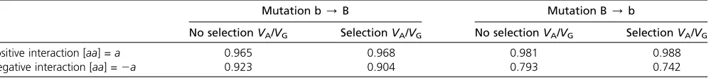
Based on diffusion equation approximations (e.g., Crow and Kimura 1970) the results should approximate those for pop-ulations with largerNvalues but similar values ofN3gene effects (or selection coefficients) for such loci, on a time scale proportional toN. We use a haploid model but approximate a diploid population of (approximate) effective sizeNh/2. The vector of gene frequency values has dimension (Nh+ 1)2, where each element specifies the probability P(i1,i2) that there are

i1 copies of the increasing allele at the first locus and i2 at the second at some generation t. The transition matrix of dimension (Nh + 1)23 (Nh + 1)2 defines conditional probabilities of joint frequency change between states. Selective values are computed assuming truncation selection on the trait being modelled, with specified selection intensity Sand selective values Sa1and Sa2, where a1and a2are the average effects (i.e., including interaction terms) in units of the phenotypic standard deviation SD (based on Robertson 1960).

Mild selection (withS= 0.29 and values ofa1anda2of 0.1 SD) was applied to represent the selection intensities when

there is both genetic variation from many loci and environmental variation. The (haploid) population size was set atNh= 40. Initial allele frequencies were set at 0.05 (2/Nh) for both loci and iteration was continued for 100 (i.e., 1.5N) generations,

i.e., close tofixation. Iteration was also undertaken with the same starting frequencies and random mating, but no selection (i.e.,S = 0). The results were computed as the average of the components of variance over the 100 generations. With positive interaction ([aa] =a), 96.8% of the genetic variation is additive with random matingvs.96.5% with selection. For negative interaction ([aa] =–a), the proportions are 94.6 and 93.3%, respectively. In the results for this two-locus case the epistatic variance has a higher proportion with negative interaction while selection seems to alter this proportion very little. Checks undertaken withNh= 20, the same starting frequency (1/20), higher intensity (S= 0.58), and fewer generations (50) gave proportions 92.9vs.92.2 for positive and 96.3vs.96.2% for negative interaction, respectively. The difference due toNis small, so the results with this order of population size serve as good indicators for the effect of selection.

In the second case, the initial frequency at locusjwas set to 1/Nh(or 1–1/Nh) (i.e., mutant in a population of sizeNh= 40) and that for locusiat the frequency distribution expected at steady state of mutation and drift without selection (i.e., U shaped) after 100 generations of random mating or selection with the selection intensity as above. With no selectionVAAis the same in all the runs, as is the additive variance in the mutated locusjwhile that for locusichanges greatly depending on the sign of the interaction [aa] of mutation due to the termpjaj[aa]ijin the formula forVA. The epistatic variance is again

highest for negative interaction, while the results with and without selection differ very little and, in general, the genetic variation is mainly additive.

In the third example the starting allele frequencies for each of the two loci were set as either 1/Nhor 1–1/Nhand the results are presented as weighted averages over these four different initial conditions. Two relative mutation rates at locus B were considered: equal, (B/b) = (b/B), and unequal, (B/b) = 3(b/B), withNh= 40. With positive interaction ([aa] =a)VA/VGaverages 98.2% for the model with equal probability and 98.5% if unequal, when there was no selection and with selection (S= 0.29) 98.3 and 98.8%, respectively. When the gene interaction is negative, these values are slightly smaller, with no selection 90.4 and 84.2%, and with selection 90.3 and 84.2%, respectively. Hence, selection produced negligible difference. In conclusion, the asymmetry in the allele frequency distributions caused by selection does not seem to alter the general picture about the proportion of epistatic variance.

Table A1 The transition matrix approach used to study the influence of genetic background on the impact of a new mutation (either with

increasing or decreasing effect) on the proportion of additive variance (VA) in the genotypic variance (VG)

Mutation b/B Mutation B/b

No selectionVA/VG SelectionVA/VG No selectionVA/VG SelectionVA/VG

Positive interaction [aa] =a 0.965 0.968 0.981 0.988

Negative interaction [aa] =2a 0.923 0.904 0.793 0.742