Suddenly Structure Mattered: Insights into Recoveries from Defaulted Debt

(1)

Today’s economy is one of the strongest in history. In 1999 alone, the S&P 500 returned nearly 20% and the GDP grew by 5.7%. Despite the idyllic economic environment, companies defaulted on their debt at a record rate in 1999. In 2000, Brand and Bahar (2000) reported that a record 75 rated or formerly rated companies in the United States defaulted on $32.4 billion of debt, and that the worldwide default rate of 2.15% was nearly twice that of 1998, surpassed only by the default rates of the 1989–1991 junk bond fallout. In the first four months of 2000 alone, more than 25 companies have filed for bankruptcy. Lenders clearly need a well-defined credit model that encompasses the various risk elements of default and recovery.

In an effort to define those elements, Portfolio Management Data (PMD), with the support of Standard & Poor’s, has created a database that tracks the value of public debt instruments' recoveries from default. (On May 3, 2000, Standard & Poor’s announced its acquisition of PMD.) The database currently contains over

1,100 publicly defaulted instruments from the period 1987 to 1996. PMD sources data from publicly filed bankruptcy and SEC filings as well as news reports. PMD appraises recoveries and, after the debt markets have had the opportunity to absorb and evaluate the instruments, adds them to the database. The database prices recoveries by valuing the instruments at three different points in the recovery process, namely, at the emergence, settlement, and liquidity events. The associated prices are:

• Emergence pricing: trading prices of pre-petition instruments at time of emergence • Settlement pricing: earliest available trading

prices of the instruments received in settlement

• Liquidity event pricing: value for illiquid settlement instruments at the time of a liquidity event, which is the event that occurs at the first date a price can be determined (such as acquisition of the company subsequent to default, refinancing,

Suddenly Structure Mattered:

Insights into Recoveries from

Defaulted Debt

Karen Van de Castle, David Keisman and Ruth Yang

This study analyses default loss experience for a sample of 690 bonds and 264 bank loans between 1987 and 1996. It is an update of a Standard and Poor’s study done one year ago that first reported that the amount of debt subordinate to an obligation has a powerful influence on that obligation’s loss in default. This paper finds that the effects of such structural features as the amount of subordinated debt and the quality of collateral have grown larger since 1990. It also finds that losses tend to be somewhat greater in the case of defaults that take longer to resolve. Statistical regression is used to estimate the separate effects of security-type collateral quality, amount of subordinated debt and time in default.

(2)

or significant rating upgrade). The database provides nominal as well as discounted recoveries (discounted by the pre-petition interest rate from last cash payment to emergence).

Since 1997, PMD and Standard & Poor’s have worked together to analyse the recovery database for insights into recovery valuation. In 1999, Van de Castle and Keisman (1999) demonstrated the “virtuous circle”—the fact that the use of increasing subordination or improved collateral leads to higher recoveries. In light of 1999’s high corporate default rate and recent analysis of the relationship between high-yield bond recoveries and seniority rankings, this update further explores the topic.

The data set (WJ Data Set) underlying this article contains 954 instruments from PMD's database, for the emergence period of 1987 through 1996. For companies that have

undergone multiple defaults, the study includes only emergence instruments that did not subsequently default within this 10-year period. Other than those recoveries for which pricing was unavailable, the WJ Data Set excludes only the default and cures, and the “time evaders”— those defaults for which firm dates of default and emergence could not be pinpointed: distressed purchases and exchanges, and restructurings. As a result of excluding these types of recoveries, the WJ Data Set is more conservative than the loss database as a whole, since all these time-evaders resulted, as would be expected, in a 100% recovery. This update approaches the topics of default and recovery with an expanded data set of defaulted instruments and looks not only at the significance of debt structure, but also at the effects of time and adversity.

The significance of structure

Ten percent of the WJ Data Set recovered less than 2% of par, 20% less than 10%, 25% less than 16%, and 50% less than 45%. (See Figure 1 for the distribution of recoveries for all instruments in the WJ Data Set.) For lenders, these are daunting recovery statistics. Moreover, if certain qualities of credits result in lower-than-average

should receive appropriate compensation for that additional risk. So how should lenders identify and manage that risk?

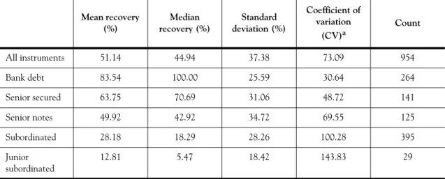
Figure 1: Distribution of present value of recoveries for all instruments in the WJ data set Instrument type is the first indicator to lenders of the risk associated with an investment. Bank loans are senior, almost always secured, and therefore less risky than senior notes, which are senior to subordinated debentures. Recovery by instrument type reinforces this industry standard. The WJ Data Set has a mean recovery for all instruments of 51.14%. (See Table 1.) However, the associated coefficient of variation (CV) is high, reflecting that the variation on the mean recovery is significant. In contrast, bank debt has a substantially higher mean recovery and a much lower CV; likewise, the statistics associated with senior secured debt show, on a diluted level, the same structural benefit of seniority. The “poor cousins” of debt structure are the senior notes and those ranked below. These instruments have a much lower mean recovery and a much higher CV. What makes these instruments different from the bank and senior secured debt above? It is the debt cushion, or the percentage of debt below the instrument, and collateral.

The average debt cushion for the all instruments in the WJ Data Set is 22.96%. Bank and senior secured debt have a higher-than-average debt cushion (48.99% and 23.94%, respectively), as would be expected, due to their senior nature. In contrast, the poor cousins have much less cushion: senior notes have an average debt cushion of 20.22%; subordinated, just 7.77%; and junior subordinated, none. While subordination does increase leverage and,

0.00% 10.00% 20.00% 30.00% 40.00% 50.00% 60.00%

(3)

therefore, risk, it also provides cushioning for the senior debt. Senior instruments such as bank loans and senior secured debt have strong recoveries—not just because they have senior claims to repayment, but also because there are other interests beneath them to absorb the fallout from default. The borrower has more cash available without affecting the senior debt’s claim to payment and collateral.

Collateral influences the quality of recoveries as much as instrument type. (See Table 2.) As would be expected, a strong correlation exists between instrument type and collateral.

However, the correlation coefficient is not strong enough to degrade the precision of estimation and, therefore, it is unnecessary to discard either of these variables. For the purposes of this analysis, collateral was separated into five classes.

Since collateral types are descriptive in nature, a multivariate regression analysis using dummy variables grouped the 17 collateral types into five classes:

• Class 1 contains the highest quality—all assets, inventories and receivables.

• Classes 2, 3, and 4 (the intermediate classes) reflect declining credit quality, liquidity and coverage.

• Class 5 represents zero assets of supporting collateral.

Then, using those five collateral classes as the dummy variables, a second regression line was created to establish, based on the degree of influence of collateral types upon recovery value, ordinal ranks. Mean recovery (%) Median recovery (%) Standard deviation (%) Coefficient of variation (CV)a Count All instruments 51.14 44.94 37.38 73.09 954 Bank debt 83.54 100.00 25.59 30.64 264 Senior secured 63.75 70.69 31.06 48.72 141 Senior notes 49.92 42.92 34.72 69.55 125 Subordinated 28.18 18.29 28.26 100.28 395 Junior subordinated 12.81 5.47 18.42 143.83 29

Table 1: Average recoveries for the WJ data set

a. Coefficient of variation: Standard deviation/average recovery: Coefficient of variation (CV) normalizes standard deviation to the mean and reflects how much deviation occurs in the data set for each additional dollar, plus or minus, of the average recovery.

Mean recovery (%) Median recovery (%) Standard deviation (%) Coefficient of variation (CV) Count All instruments 51.14 44.94 37.38 73.09 954

Class 1: all assets, inventory, and receivables

85.13 100.00 24.85 29.19 160

Class 5: unsecured 33.78 24.65 32.08 94.95 569

(4)

As expected, as the quality of the collateral supporting the security diminishes, the percent recovery declines. Furthermore, a significant difference in recovery value exists between instruments secured with any type of collateral and those without collateral. The mean recovery for collateral type Class 4, which encompasses collateral with extremely low potential for significant liquidation value, is 61.93%, nearly twice that of Class 5, which is unsecured. The analysis makes it clear that some collateral—any collateral—is better than no collateral.

The combined impact on structure, of debt cushion and collateral quality, is equally

apparent. (See Table 3.) Not only do greater debt cushions increase mean recoveries and decrease corresponding CVs, but excluding unsecured instruments from a cohort further reduces the potential for loss.

The improvement of mean recoveries with increased debt cushion and collateral quality clearly reinforces the importance of what seems obvious: the virtuous circle. However, is this an age-old theorem or a lesson of time?

Lesson in a bottle

The defaults of 1999 necessitate the

continuation of the search for new insights into recovery values, and for a model to predict a lender's potential loss given default of an

instrument. In particular, what is the influence of time in default—the period between the last cash payment and emergence? Furthermore, have changes in debt structuring occurred over time, from 1987 through 1996? Results indicate that not only is time in default significantly correlated

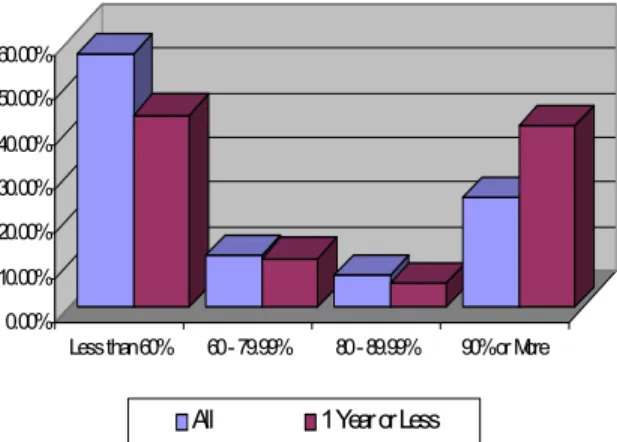
with the value of recovery (Table 4), but that emergence within the first year of default is the most rewarding. Figure 2 contrasts the recovery dispersion data for all default time lengths with those that lasted a year or less. The chart shows clear evidence of the benefits of a short recovery period. Evidence also indicates, however, that emergence after the first year of default is much more expensive today than it was 10 years ago.

Figure 2: Time in default—all periods versus one year or less for WJ data set

Lending as an institution and loans as financial instruments have changed dramatically since 1980. The innovative mechanics of the junk bond kingdom, which created and financed the excesses of leveraged buy-out (LBO) frenzy, amazed the financial markets of the early 1980s. Debt financing occurred on a scale the size of which had never been seen before. Twenty-five billion dollars of debt was issued to finance the LBO of one company—RJR Nabisco. The subsequent collapse, however, of Drexel Burnham's house of cards, in conjunction with

Mean recovery (%) Median recovery (%) Standard deviation (%) Coefficient of variation (CV) Count All instruments 51.14 44.94 37.38 73.09 954 50% or greater debt cushion 82.55 100.00 28.22 34.18 184 50% or greater debt cushion and any type of collateral

89.84 100.00 18.62 20.72 151

Table 3: Value of structuring the WJ data set

0.00% 10.00% 20.00% 30.00% 40.00% 50.00% 60.00%

Less than 60% 60 - 79.99% 80 - 89.99% 90% or More

(5)

some precipitous downturns in the stock market, caused many companies, most of them highly leveraged, to default on their debt at an

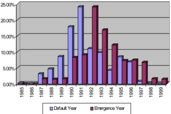
unprecedented rate during 1990 and 1991. (See Figure 3.)

Figure 3: Timing of defaults and emergences for WJ data set

The 10 largest bankruptcies in the database total $22.03 billion and include Federated

Department Stores, R.H. Macy, Southland and Charter Medical. Eight of those defaults ($17.41 billion) occurred from 1989 to 1991. (R.H. Macy held out until January 1992.) The junk-bond tumult of the 1980s contributed to debt defaulting on an unprecedented scale.

Consequently, the fear pervaded the market that

all the multimillion-dollar-fee mega-LBOs hovered on the edge of default, and the leveraged loan market nearly shut its doors. Arrangers as well as lenders received a crash course in bankruptcy. As a result, only well-structured deals made it to market. Suddenly structure mattered.

In analysing the effects of time and economic events, the WJ Data Set was split into two cohorts based upon date of emergence. Using the emergence date of December 31, 1990 as the dividing point allows each cohort to pick up a relatively even number of defaults resulting from the three primary economic shocks of the period: the 1987 stock market crash, the collapse of Drexel Burnham and the junk bond market, and the 1990 stock market crash. The data in Table 5 indicate no significant difference between the two time-period cohorts. Analysis of the components of structure, however, reveals developments in the relevance of collateral and debt cushion.

Prior to 1991, lenders primarily received recovery benefit from only one component of structure: instrument type (as indicated by the strong t-statistic associated with the instrument variable in Table 6). Collateral and debt cushion failed to

One year or less 64.87 77.34 36.68 56.54 241

More than a year 46.49 39.67 36.48 78.47 713

Table 4: The price of time for the WJ data set

0.00% 5.00% 10.00% 15.00% 20.00% 25.00% 1985 1986 1987 1988 1989 1990 1991 1992 1993 1994 1995 1996 1997 1998 1999

Default Year Emergence Year

1990 & prior cohort 42.28 33.04 34.20 80.89 124

1991 plus cohort 53.40 50.93 37.80 70.42 829

(6)

influence structure in any predictable fashion; their corresponding t-statistics indicate no significant effects on recovery. In contrast, the statistics for the period 1991 and beyond reveal an increased importance of subordination and collateral. In this cohort, greater debt cushion improves recoveries; lesser-quality collateral weakens recoveries. It appears that the tremendous bankruptcies of the 1990–1991 period taught the debt markets a brutal lesson on the importance of all elements of structure. In addition, beginning in 1991, time in default had increased significance; each year in default had an obvious price.

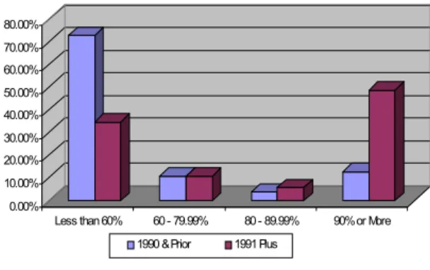
Table 7 demonstrates that a short time in default benefits today's lender significantly more than the 1980s' investor: The average recovery for defaults of a year or less is 80% greater and has a tremendously lower variation. Furthermore, Figure 4 indicates, in the 1990 and prior group, the dispersion of recoveries that spent a year or less in default does not significantly differ from

the dispersion for all time periods. However, for the “1991 and Beyond” set, the dispersion of recoveries of a year or less in default is almost the inversion of the total distribution: 49% of the cohort recovered at least 90%. Time matters much more in today's fast-paced world of debt structure, and the legal and financial players in the bankruptcy world recognize this.

Figure 4: Dispersion of recoveries on defaults of one year or less for WJ data set

1990 and prior 1991 and beyond

Coefficient t-statistica Coefficient t-statistic

Intercept 51.14 44.94 37.38 73.09 Instrumentb type 953.3574 6.2343 961.2794 25.1891 Collateral (169.1919) (5.4116) (81.4329) (8.1235) Time in default 3.8704 0.1403 (43.3961) (5.7193) Debt cushion (32.6935) (0.2109) 300.2926 7.1772 Principal default (0.0000) (0.4304) 0.0000 1.5418 R-Squared 0.3919 0.4789 Adjusted R-Squared 0.3661 0.4758 Observations 124 830

Table 6: Multivariate linear regression statistics for the two time periods for WJ data set

a. t-statistic: ratio of standard error to variable coefficient. A higher t-statistic reflects less variation to the coefficient. The t-critical, minimum t-statistic, for a one-tailed population greater than 120 with a 5% confidence interval is 2.58.

b. As noted before, instrument type is ranked from most to least senior: bank debt, senior secured, senior notes, subordinated, junior subordinated. The analysis employed dummy variables to verify the ordinal ranking of the instruments.

0.00% 10.00% 20.00% 30.00% 40.00% 50.00% 60.00% 70.00% 80.00%

Less than 60% 60 - 79.99% 80 - 89.99% 90% or More 1990 & Prior 1991 Plus

(7)

That was then, this is now

The LBO defaults of the late 1980s—

unprecedented in terms of volume and size—sent a shock waves through the system, affecting both arrangers and lenders. On one side, the defaults showed underwriters how sound debt structuring provided protection to potential lenders/investors in the event of default. On the other side, the defaults showed lenders the characteristics of sound structuring. Whereas the defaults of the 1990–1991 period slowed the growth of the debt market, the knowledge gained from cleaning up after these defaults helped lenders regain their confidence. The mid-1990s experienced a return to debt financing, even in light of the seemingly never-ending boom of equity markets. This bull market provided fuel for the tremendous growth of the debt markets and shaped the recoveries from the junk bond debacle of the 1980s.

In the past decade, risk analysts have developed resources to help lenders analyse default triggers and events. Databases and statistical models are available to evaluate past events in a better effort to predict future risks. The methodologies also continually remind lenders not only to analyse new events, but also, in light of the ever-changing present, to revisit the past to develop new

perspectives and insights into credit risk. Rising interest rates and shrinking profit margins will not only provide the industry with new default events

to analyse, but also with new frameworks in which to review existing information.

PMD is in the process of adding the recoveries of the past three years to its loss database, providing a wealth of new opportunities to improve our understanding of debt instruments. Just as this examination of PMD's information on the first cycle of defaults has provided significant insight into the relevance and mechanics of structure, continual analysis will only improve the debt market's ability to manage credit risk. With tools such as PMD's loss database, financial

institutions can look at the full cycles of

companies and examine debt instruments from a number of perspectives including date of credit issue, industry, ratings and many other variables. These lessons will help lenders to moderate potential losses through improved capital allocation, pricing and risk management. Today's free flow of information and analytical tools provide lenders with tools for better management of the risks associated with default and recovery.

References

Brand, L. and R. Bahar, 2000, “Greater risk means more defaults in 1999,” Ratings Performance 1999—Stability & Transition, Standard & Poor’s, February.

Van de Castle, K. and D. Keisman, 1999, “Recovering your money: insights into losses from defaults,” Ratings Direct, Standard & Poor’s, August.

1990 and prior 1991 and beyond

Recovery (%) Coefficient of

variation (CV) Recovery (%)

Coefficient of variation (CV)

One year or less 39.65 82.66 71.44 48.65

Between 1 and 2 years 45.21 80.09 52.32 68.27

More than 4 years _N/Aa _N/Aa _48.36 _88.49

More than a year 44.37 79.76 46.71 78.45

Table 7: Average recoveries by time in default: 1990 and prior versus 1991 and beyond for WJ data set

(8)