Vol. 13, No. 1, 2020, 144-157
ISSN 1307-5543 – www.ejpam.com Published by New York Business Global
Numerical methods for advection problem
Diog`ene Vianney Pongui Ngoma1, Germain Nguimbi1∗, Vital Delmas Mabonzo2, Narcisse Batangouna1
1 Ecole Nationale Sup´erieure Polytechnique, Marien Ngouabi University, Congo 2 Parcours Math´ematiques, E.N.S, Marien Ngouabi University, Brazzaville, Congo
Abstract. This paper aims is to solve an advection problem whereu=u(x, t) is the solution by Lax-Wendrof and finite difference methods, to study the analytical stability inL2[0,1], L∞[0,1], then calculate the truncation error of these methods and finally study the analytical convergence of these methods. These numerical techniques of resolution were implemented inScilab.
2020 Mathematics Subject Classifications: 65M06, 65M12, 65K05, 65L12
Key Words and Phrases: Advection problem, truncation error, stability, convergence, Lax-Wendroff and finite difference methods
1. Introduction
Many disciplines of physics consist of describing phenomena of transport, heat and induction. To describe such phenomena, it seems quite natural to describe the evolu-tion of certain physical quantities in time as well as in space. Since they involve several parameters, the differential equations involve partial derivatives with respect to each pa-rameter. Hence the term ”partial differential equations ” in short PDEs. The PDEs are also involved in the mathematical study of many problems encountered in various fields of science (mechanics, chemistry, economics, biology, etc.), as well as in various applied fields, or even advanced industrial, mainly in engineering and oil industry.
A PDE in itself does not have a pure solution, because in general it is difficult to find a solutionuto it in a unique way with no limit condition [1–3, 5, 8, 11]. After modeling a physical problem (a visible problem) we get an invisible problem (a mathematical equation: partial differential equations for example), but PDEs are usually very complex to solve, or they have solutions for particular cases, but also the random phenomena of nature lead to nonlinear equations which gives a complexity to the mathematical model studied.
The principle of solving partial differential equations is to replace a complex system into a simple object or operator by leaving the main aspects of the original, which is called
∗
Corresponding author.
DOI: https://doi.org/10.29020/nybg.ejpam.v13i1.3619
Email addresses: [email protected](D.V. Pongui Ngoma),
[email protected](G.Nguimbi),[email protected](V. D. Mabonzo)
a numerical resolution. We want to solve the advection problem of order one in time and space (1) of solutionu=u(x, t) by finite difference and Lax-Wendroff methods [4–6, 9, 10].
∂u ∂t +α
∂u
∂x = 0, (1)
whereα is the advection coefficient, subject to the homogeneous Dirichlet conditions
u(0, t) =u(1, t) = 0,
going from the initial solution
u(x,0) =u0(x) =sin(19πx).
These methods will have to calculate the solution u of the problem for different steps in space and time in order to represent on the same graph the numerical solutions of the finite difference and Lax-Wendroff methods for the equation (1), we will study the analytical stability inL2([0,1]) andL∞([0,1]) of finite difference and Lax-Wendroff methods for the advection equation, then we will calculate the truncation error of these methods. We will study the analytical convergence of each of these methods.
All these numerical methods will be implemented with theScilabsoftware.
2. Advection problem
The advection or linear transport equation is a hyperbolic PDE, it is the simplest one and consists in finding the solution u=u(x, t) ∈Rsuch that [8]
∂u ∂t +α
∂u
∂x = 0, (2)
whereα >0 is the advection coefficient.
For the purpose of the resolution we will consider the homogeneous Dirichlet boundary conditions
u(0, t) =u(1, t) = 0.
And the solution is initiated from u(x,0) =u0(x) =sin(19πx).
3. Numerical resolution of advection problem
In this section, we will calculate the solution of the advection model by using two numerical methods including the finite difference method and that of Lax-Wendroff.
3.1. Resolution by the finite difference method
We shall now calculate the solutionu(x, t) of the advection problem for different steps in space and time. For this purpose, the finite difference scheme of the advection problem is written:
unj+1−unj
∆t +α
unj −unj−1
and in the form of recurrence
unj+1 =βunj−1+ (1−β)unj , with β=α∆t
∆x (4)
The homogeneous Dirichlet boundary conditions are
u(0, t)'u(x0, tn) =un0 = 0, u(1, t)'u(xN+1, tn) =unN+1 = 0,
By varying the index j= 1,2,3, . . . , N of the equation (4), we obtain:
un1+1
un2+1
un3+1
.. .
unN+1 =
1−β 0 0 . . . 0
β 1−β 0 . . . 0
0 β 1−β . . . 0
..
. . .. . .. ...
0 0 . . . β 1−β un 1
un2
un3
.. . un N (5)
3.2. Resolution by Lax-Wendroff method
We will calculate the solution u(x, t) of the advection problem for different steps in space and time. For this purpose, the Lax-Wendroff scheme for the advection equation is written as follows
unj+1−unj
∆t +c
un
j+1−unj−1
2∆x −
c2∆t
2
un
j−1−2unj +unj+1
∆x2 = 0 (6)
and in the form of recurrence
unj+1 = (1−λ2)unj +
λ2 2 + λ 2
unj−1+ λ2 2 − λ 2
unj+1, avec λ=c∆t
∆x. (7)
The homogeneous Dirichlet boundary conditions are
u(0, t)'u(x0, tn) =un0 = 0, u(1, t)'u(xN+1, tn) =unN+1 = 0,
un1+1
un2+1
un3+1
.. .
unN+1 =
(1−λ2) (λ2
2 − λ
2) 0 0 · · · 0
(λ22 +λ2) (1−λ2) (λ22 −λ
2) 0 · · · 0
0 (λ22 + λ2) (1−λ2) (λ22 −λ 2)· · ·0
..
. . .. . .. (λ22 −λ
2)
0 · · · 0 (λ22 +λ2) (1−λ2)
un1
un2
un3
.. .
unN (8)
Solving the advection problem by the finite difference and Lax-Wendroff methods, we find that the linear system obtained by the finite difference method admits a bidiagonal and non-symmetric while that obtained by Lax-Wendroff is tridiagonal and non-symmetric.
3.3. Numerical simulation
(a) (b)
(c)
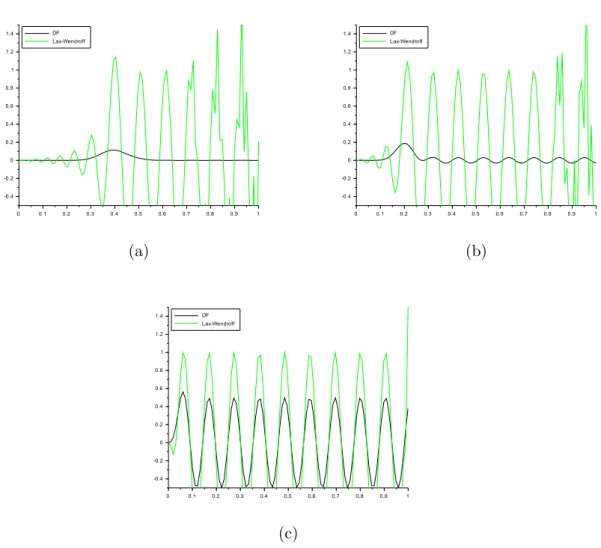
Figure 1: Representation of the solution of the advection problem by finite difference (FD) and Lax-Wendroff methods forN= 99 et T = 2000.
• Taking α = 0.2 et ∆t = 0.001, we note that the solution obtained by the finite difference (FD) method remains constant whereas that obtained by the Lax-Wendroff method is unstable at first, then becomes stable and becomes unstable after (Figure 1 a).
• Taking α = 0.002 et ∆t = 0.05, we find that the solution by FD is constant at the beginning, then oscillates at very low amplitudes whereas by Lax-Wendroff it is unstable at first, then remains stable for a long time and becomes unstable after ( Figure 1 b ).
• Taking α = 0.02 et ∆t = 0.001, we note that both solutions (FD and Lax-Wendroff) converge and the solution by Lax-Wendroff admits a higher peak than that obtained by FD ( Figure 1 c ).
(d) (e)
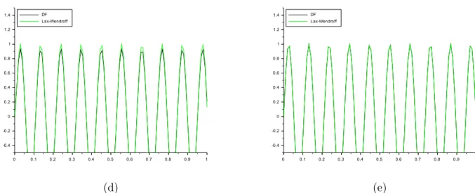
Figure 2: Representation of the solution of the advection problem by finite difference (FD) and Lax-Wendroff methods forN= 99 et T = 2000.
• Taking α = 0.002 et ∆t = 0.001, we find that both solutions (FD and Lax-Wendroff) converge numerically almost everywhere ( Figure 2 d ).
• taking α = 0.002 et ∆t = 0.000001, we see that both solutions (FD and Lax-Wendroff) admit a total convergence numerically( Figure 2 e)
4. Study of the analytical stability in L2([0; 1]) and L∞([0; 1]) of the finite
difference and Lax-Wendroff methods for the advection equation
In this section, we study the analytical stability inL2([0; 1]) andL∞([0; 1]) of the finite difference and Lax-Wendroff methods for the advection equation
4.1. Analytical stability in L2([0; 1]) for the finite difference method of the transport equation
Here, we will study the analytical stability inL2([0; 1]) of the numerical finite difference method used for the advection problem.
Leteiwx andeiwxj be the mode values of the exact and discrete operators respectively
whereiis the imaginary unit such that i2 =−1.
Let un = un
weiwx, i ∈ C and xj = j∆x ' jh where h = ∆x is the constant step of space discretization.
Then
unj =unweiwxj 'un
weiwjh (9)
Replacing (9) in (4) , we obtain
unw+1eiwjh=βunweiwjh.e−iwh+ (1−β)unweiwjh, (10)
unw+1 = [βe−iwh+ (1−β)]unw , wh∈[−π;π] (11) Let us put r(wh) = βe−iwh+ (1−β), where r(wh) is the amplification coefficient of the finite difference operator .
Let us show that |r(wh)|61 ,
r(wh)2 = 1−2β+ 2βcoswh−2β2coswh+β2+β2 ,
= (1−β)2+β2+ 2βcoswh(1−β),
= (1−β)2+ 2β(1−β)coswh+β2 ,
|r(wh)|2 =|(1−β)2+ 2β(1−β)coswh|+β2 ,
|r(wh)|2 6(1−β)2+ 2β|(1−β)|+β2= [(1−β) +β]2 61,
where
|r(wh)|61.
4.2. Analytical stability in L2([0; 1]) for the Lax-Wendroff method of the transport equation
We shall want to study the analytical stability inL2([0; 1]) of the Lax-Wendroff method used for the advection problem. Thus let us use the Von-Neuman condition.
The Lax-Wendroff scheme for the advection equation is
unj+1=unj −λu n
j+1−unj−1
2 +λ
2u n
j−1−2unj +unj+1
2 .
According to the Von-Neumann stability criterion:
A= u n+1
un (12)
un+1 un =
unj − λ2(unj+1−unj−1) +λ22(unj−1−2unj +unj+1)
un ,
= ( λ2
2 + λ
2)unj−1+ (1−λ2)unj + (λ 2
2 − λ 2)unj+1
un .
Let us take two mode values of the exact and discrete operators eik∆x and eikj∆x re-spectively.
Let be
unj =eikj∆xunk
Equation (12) then becomes
A= ( λ2
2 + λ 2)u
n k.eik(j
−1)∆x+ (1−λ2)un
k.eikj∆x+ (λ 2
2 − λ 2)u
n
k.eik(j+1)∆x un
k.eikj∆x
,
= ( λ2
2 + λ 2)u
n
k.eikj∆xe
−ik∆x+ (1−λ2)un
k.eikj∆x+ ( λ2
2 − λ 2)u
n
k.eikj∆xeik∆x un
k.eikj∆x
,
=
h
(λ22 +λ2)e−ik∆x+ (1−λ2) + (λ22 −λ 2)e
ik∆xiun k.eikj∆x un
k.eikj∆x
.
After simplification, we obtain
A=λ2cos(k∆x)−iλsin(k∆x) + 1−λ2 , A= 1−λ2[1−cos(k∆x)]−iλsin(k∆x).
By taking the semi-norm ofA
|A|2 =1−λ2[1−cos(k∆x)] 2
+λ2sin2(k∆x),
|A|61,
because
1−λ2>0 , λ261.
Thus, the scheme is stable in theL2([0,1]) norm for the Lax-Wendroff method of the CFL transport equationλ61 [4, 8].
4.3. Analytical stability in L∞([0; 1]) for the finite difference method of the transport equation
We may now study the analytical stability inL∞([0; 1]) of the finite difference method used for the advection problem.
Let us then use, the maximum principe.
Considering the linear interpolation between unj−1 and unj of the equation (4), we then get
unj+1=βunj−1+ (1−β)unj 6max j∈Z
(unj−1, unj), Therefore :
unj+1 6max j∈Z
(unj−1, unj).
By passing to semi-norm and supremum, we obtain
|unj+1|6max j∈Z
(|unj−1|,|unj)|),
sup|unj+1|6sup max j∈Z(|u
n
j−1|,|unj)|),
kun+1k∞6kunk∞ .
By simple recurrence, we have
forn= 0, ku1 k∞6ku0 k∞
forn= 1, ku2 k∞6ku1 k∞6ku0k∞ forn= 2, ku3 k∞6ku2 k∞6ku0k∞
.. .
at rankn, kunk∞6ku0k∞=C Then
kunk∞6C (C constant).
4.4. Analytical stability in L∞([0; 1]) for the Lax-Wendroff method of the transport equation
We may now study the analytical stability inL∞([0; 1]) of the finite difference method used for the advection problem. we may then use the maximum principe.
Considering the linear interpolation between un
j−1, unj and unj+1 of the equation (7), we
have:
unj+1= (1−λ2)unj +
λ2
2 +
λ
2
unj−1+
λ2
2 −
λ
2
unj+1 6max j∈Z
(unj−1, unj, unj+1),
Therefore
unj+16max j∈Z
(unj−1, unj, unj+1).
By passing to semi-norm and supremum, we obtain
|unj+1|6max j∈Z(|u
n
j−1|,|unj|,|unj+1|),
sup|unj+1|6sup max j∈Z
(|unj−1|,|unj|,|unj+1|),
kun+1k∞6kunk∞ .
by simple recurrence, we have
forn= 0, ku1 k∞6ku0 k∞
forn= 1, ku2 k∞6ku1 k∞6ku0k∞ forn= 2, ku3 k∞6ku2 k∞6ku0k∞
.. .
at rankn, kunk∞6ku0k∞=C.
Which proves the analytical stability in L∞([0; 1]) for the Lax-Wendroff method of the transport equation.
5. Analytical convergence of numerical methods
5.1. Truncation error for the finite difference method of the transport equation
Using Taylor’s development of order 2 in relation with time to approach ∂u∂t,we obtain
u(xj, tn+1)−u(xj, tn)
∆t =
∂u
∂t(xj, tn) +
∆t
2!
∂2u
∂t2(xj, tn) +O(∆t
2). (13)
To approach the derivative ∂u∂x, let us use Taylor’s development of order 2 in relation to space. We then obtain
αu(xj, tn)−u(xj−1, tn)
∆x =α
∂u
∂x(xj, tn)−α
∆x
2!
∂2u
∂x2(xj, tn) +O(∆x
2) (14)
We then define the truncation error of the transport equation for the finite difference method by
ζjn= u(xj, tn+1)−u(xj, tn)
∆t +α
u(xj, tn)−u(xj−1, tn)
∆x . (15)
By adding the equations (13) and (14) member to member, we get
ζjn= ∂u
∂t(xj, tn)+α ∂u
∂x(xj, tn)+
∆t
2!
∂2u
∂t2(xj, tn)−α
∆x
2!
∂2u
∂x2(xj, tn)+O(∆t
2+∆x2)
(16) knowing that
∂u
∂t(xj, tn) +α ∂u
∂x(xj, tn) = 0,
as a result
ζjn= ∆t 2!
∂2u
∂t2(xj, tn)−α
∆x
2!
∂2u
∂x2(xj, tn) +O(∆t
2+ ∆x2).
We obtain a truncation error of the equation of transport of order 2 in space and in time.
Expressing ∂∂t2u2 in terms of ∂2u
∂x2, the truncation error is written
ζjn= ∆t 2!α
2∂2u
∂x2(xj, tn)−α
∆x
2!
∂2u
∂x2(xj, tn) +O(∆t
2+ ∆x2),
ζjn= α
2(α∆t−∆x)
∂2u
∂x2(xj, tn). (17)
Study of the consistency
According to our analysis, the truncation error is
ζjn= α
2(α∆t−∆x)
∂2u
∂x2(xj, tn).
Doing
(∆x,∆t)−→(0,0) Therefore
ζjn−→(0,0).
Which proves the consistency of the finite difference scheme for the transport equation.
Since the scheme is stable and consistent, it is concluded that the numerical solution of unj of the finite difference scheme for the transport equation is convergent.
5.2. Truncation error for the Lax-Wendroff method of the transport equa-tion
The Lax-Wendroff scheme for the advection equation is written as
unj+1−unj
∆t +c
unj+1−unj−1
2∆x −
c2∆t
2
un
j−1−2unj +unj+1
∆x2 = 0. (18)
The truncation error of the transport equation for the Lax-Wendroff method is defined by
ζj0n= u(xj, tn+1)−u(xj, tn)
∆t +c
u(xj+1, tn)−u(xj−1, tn)
2∆x −
c2∆t
2
u(xj+1, tn)−2u(xj, tn) +u(xj−1, tn) ∆x2
(19) Let us make a development of Taylor inx around the point xj and int around the point tn. Since u is the solution of the transport equation (1), we have
u(xj, tn+1)−u(xj, tn)
∆t =
∂u
∂t(xj, tn) +
∆t
2!
∂2u
∂t2(xj, tn) +O(∆t
2), (20)
cu(xj+1, tn)−u(xj−1, tn)
2∆x =c
∂u
∂x(xj, tn), (21)
c2∆t
2
un
j−1−2unj +unj+1
∆x2 =
c2
2
∆t∂ 2u
∂x2(xj, tn). (22)
By inserting the relations (20), (21) and (22) into the expression of ζj0n, we get
ζj0n= ∆t 2!
∂2u
∂t2(xj, tn)−
c2
2
∆t∂ 2u
∂x2(xj, tn) +O(∆t
The truncation error for the Lax-Wendroff method of the transport equation can be written
ζj0n= ∆t 2
∂2u
∂t2(xj, tn)−c 2∂2u
∂x2(xj, tn)
+O(∆t2+ ∆x2),
= ∆t 2
c2∂
2u
∂x2(xj, tn)−c 2∂2u
∂x2(xj, tn)
+O(∆t2+ ∆x2),
ζj0n=O(∆t2+ ∆x2).
We obtain a truncation error depending on ∆t and ∆x.
Study of the consistency
Here it is easier to see that the truncation error of the transport equation for the Lax-Wendroff schem is zero. We can directly deduce the consistency of the schem because it is obvious thatζj0n−→(0,0) when (∆t,∆x)−→(0,0).
Therefore the numerical solution of unj of the Lax-Wendroff scheme for the transport equation is convergent.
6. Conclusion
The work proposed in this paper allowed us not only to highlight the finite differ-ence and Lax-Wendroff methods, but also to discover the importance of these methods in the numerical resolution of the advection problem. In this paper, we performed a numerical resolution of the advection problem using finite difference and Lax-Wendroff methods. Thus, we obtained linear systems whose matrices are bidiagonal non-symmetric (Finite Difference method), non-symmetric tridiagonal for Lax-Wendroff method. Then we proved that the numerical convergence between these solutions is total by taking:
α = 0.002, ∆t = 10−6, N = 99 and T = 2000. In addition, we used the
Von-Neumann and CFL conditions to prove the analytical stability of the solution unj of the advection equation from the finite difference and Lax-Wendroff schemes. Finally, we have also proved the analytical convergence of the solution un
j using the truncation error of these methods.
Acknowledgements
References
[1] H. Beghr and G. Harutjunjan,Robin boundary value problem for the Poisson equation, J. Anal. Appl., 4, 29-45, 2006.
[2] Bourchra Bensiali, Guillaume Chiavassa, and Jacques Liandrat.Penalization of Robin Boundary conditions, Applied Numerical Mathematics, 96, 134-152, 2006.
[3] Shao-Gao Deng.Positive solutions for Robin problem involving the p(x)-Laplacian, J. Math. Anal. Appl., 360,548-560, 2009
[4] Marc Ethier and Y. Bourgault.Semi-implicit time-discretization schemes for the bido-maine model.SIAM .J. Numer. Anal. 46: 2443-2468, 2008.
[5] M. Hinze, R. Pinnau, M. Ulbrich, and S. Ulbrich. Mathematical modelling: Theory and Applications. Springer, 2009.
[6] Peter Knabner, and Lutz Angermann. Numerical methods for elliptic and parabolic partial differential equations,(2nd ed.) Springer, 2000.
[7] Loredana Lanzani, and Osvaldo M´endez . The Poisson’s problem for the Laplacian with Robin boundary condition in non-smooth domains, Rev. Math. Iberoamericana, 22, 181-204, 2006.
[8] Brigitte Lucquin. Equations aux drives partielles et leurs approximations, Ellipses, 2004.
[9] G. Nguimbi, D. V. Pongui Ngoma, V. D. Mabonzo, B. B. B. Madzou and L. G. Ngoma BouangaMathematical and numerical analysis for Neumann boundary value problem of the Poisson equation,Journal of advnces in mathemtics and computer science, 30, 1-13, 2019.
[10] G. Nguimbi, D. V. Pongui Ngoma, V. D. Mabonzo, B. B. B.Madzou and M. J. J. Kokolo On the existence, uniqueness and application of the finite difference method for solving Robin elliptic boundary value problem,Journal of mathematics research, 11, 26-36, 2019.