Vol. 12, No. 3, 2019, 1052-1068 ISSN 1307-5543 – www.ejpam.com Published by New York Business Global
Geostatistical analysis with copula-based models of
madograms, correlograms and variograms.
Fabrice Ouoba1, Diakarya Barro2,∗, Hay Yoba Talkibing1
1 LANIBIO, UFR-SEA, Universit´e Ouaga 1, Pr JKZ, Burkina Faso 2 UFR-SEG, Universit´e Ouaga 2, Burkina Faso
Abstract. This paper investigates models of stochastic dependence with geostatistical tools. Specifically, we use copulas to propose new models of stochastic spatial tools such as variograms, correlograms and the madograms. Copula versions of covariograms are provided both in second stationnary and intrinsic frameworks. Moreover, some usual families of models of variograms are clarified with the corresponding parameters
1. Introduction
Spatial statistics focus on phenomena whose observations is a random process Z =
{Zs, s∈S} indexed by a spatial set S = {s1, . . . , sn} while Zs denotes a geographical space D. Such technics where developed first in geostatistics more specifically from the for geologists. Geostatistics are applications of probabilistic analysis methods to the study of phenomena that extends into space and present a structuration. Here, space refers to be the geographical space, but it may be the temporal axis or more abstract spaces. To quantify this structure, the geostatistical tools used are mainly the variogram, the correl-ogram and the madcorrel-ogram depending on the type of sampled data.
While modelling spatial extreme variability of an isotropic and max-stable field, Cooley et al. (2006) have introduced the F-madogramγF(h) defined by
γF(h) = 12E{|F(Z(s))−F(Z(s+h))|}. (1) where h is the average value of the separating distance between the two points. This tool provides a generalization of the so called λ-madogram associated to the distribution underlying the stochastic process, such as:
γF(h) = 12E n
[F(Z(s))] λ−
[F(Z(s+h))]1−λ o
;λ∈]0,1[. (2)
∗
Corresponding author.
DOI: https://doi.org/10.29020/nybg.ejpam.v12i3.3389
Email addresses: [email protected] (O. Fabrice)
[email protected] (B. Diakarya),[email protected] (H. Y. Talkibing)
The variogram or the semi-variogram makes it possible to determine whether the distri-bution or parameters studied have a structure, random or periodic. Its representation has three characteristic properties: the nugget effect, the range and the sill. The nugget effect characterizes the variability at the origin. The sill, if it exists, is characterized by the attainment of a plateau where the semi-variogram become constant with the evolution of h and the range which characterizes the limiting distance of spatial structuring.
The correlogram function is identical to the linear coefficient between a series of spatial data. It’s given by:
ρ(s1, s2) =corr(Z(s1), Z(s2)) =
cov(Z(s1), Z(s2))
σs1σs2
. (3)
It is possible to express graphically the correlation between two variables by mean of their separate distance h. In particular, for spatial extreme or spatial temporal phenomena, geostatistical tools such as the variogram or correlogram are not appropriate for studying the spatial structuring of data.
Typically, the madogram or variogram of the first order is used to characterize this spatial structure of the extreme data. Such as, for all separating distance h,
M(h) = E(|Z(s+h)−Z(x)|
2 . (4)
While studying spatial models of extreme values, Barro et al.[2] have considered a set of locations S = {x1, ..., xs} ⊂R2, where the process is observed. If Yk,1;...;Yk,s denote independent copies from the second-order stationary random field, for k = 1, ..., n, they poined out that every spatial univariate marginal laws lies in the domain of attraction of the real-value parametric Generalized extreme value (GEV) distribution, defined spatially on the subdomain:
Sξ={xi ∈S;σi(xi) +ξi(xi) (yi(xi)−µi(xi))>0} ⊂S,
such as:
GEV (yi(xi)) =
exp
−h1 +ξi(xi)
yi(xi)−µi(xi)
σi(xi)
i −1
ξi(xi)
if ξi(xi)6= 0 expn−expn−yi(xi)−µi(xi)
σi(xi)
oo
if ξi(xi) = 0
; (5)
where the parameters {µi(xi)∈R}, {σi(xi)>0} and {ξi(xi)∈R} are referred to as
the spatial version of location, the scale and the shape parameters for the site xi respec-tively.
madogram of spatial variable are modeled via the copula underlying their joint distribu-tion. Specifically, section 2 gives the background tools of stochastic analysis that turn to be necessary, while section 3 deals with our main results, copulas versions of variogram, madogram, covariogram and correlogram via copulas.
2. Preliminaries
This section summaries definitions and properties on the copulas of multivariate joint processes dependence which turn out to be necessary for our approach. For this purpose the definition of multivariate copula is necessary. Moreover, we provide a survey of the main geostatistical tools used in this paper.
2.1. Some geostatistical tools in spatial dependence
The covariance of a random field measures the strength of the relationship witch exists between the random variables witch represents it in the different observation sites. It is defined onRd×Rd inR,f or all (s1, s2)∈Rd×Rd,
c(s1, s2) =Cov[Z(s1), Z(s2)] =E[Z(s1)Z(s2)]−m(s1)m(s2).
Since,
E[Z(s1)Z(s2)] =
Z +∞ −∞
Z +∞ −∞
z1z2h(s1, s2)dz1dz2,
the covariance function can still be written such as:
c(s1, s2) =
Z +∞ −∞
Z +∞ −∞
z1z2h(s1, s2)dz1dz2−m(s1)m(s2)
where m(s1) is the mean of Z(s1) and h(s1, s2), the joint density function of Z(s1) and
Z(s2). The Cauchy-Schwarz inequality links the covariance between Z(s1) and Z(s2) to
the variance of Z(s1) and Z(s2),
Cov[Z(s1), Z(s2)]| ≤
p
V ar[Z(s1)]V ar[Z(s2)].
The madogram of a random field, especially used in the extreme case, determines the strength of the relationship between the random variables that represents it in the different observation sites. It is set to Rd inR+ by:
∀h∈Rd, M(h) = E(|Z(s1+h)−Z(s1)|)
2 ; ∀s1 ∈R
d.
2.2. A Survey of Copulas Functions
Copulas functions can be used to describe the dependence of variables or for spatial interpolation. The copula were introduced by Sklar [10] in order to characterize a vector
of continuous multivariate distributions F to marginalF1, . . . , Fd, there is a copula function C such that
F(s1, . . . , sn) =C[F1(s1), . . . , Fd(sd].
Definition 1. An n-dimensional copula is a distribution function Cn : [0,1]n −→ [0,1] satisfying the following properties.
i) C(u) = 0 if one of the coordinates of u is zero, that is
Cn(u1, ..., ui−1,0, ui+1, ..., un) = 0; f or, all(u1, ..., ui−1, ui+1, ..., un)∈[0,1]n−1.
ii)
Cn(u1, ..., ui−1,1, ui+1, ..., un) =Cn−1(u1, ..., ui−1, ui+1, ..., un), , an (n-1) copula for all i.
iii) The volume VB of any rectangle B = [a, b]⊆[0,1]n is positive, that is,
VB([a, b]) = ∆bann∆
bn−1
an−1. . .∆
b1
a1C(u) =
Z B
dCn(u1, ..., un)≥0. (6)
where,
∆bk
akC(u) =C(u1, . . . , uk−1, bk, uk+1, . . . , un)−C(u1, . . . , uk−1, ak, uk+1, . . . , un)≥0.
The use of copulas in stochastic analysis whas justified by the canonical parametriza-tion of Sklar, see Joe [9]or Nelsen [12], such that the n-dimensional copula C associated to a random vector (X1, ..., Xn) with cumulative distribution F and with continuous marginal
F1, ..., Fn is given, for (u1, ..., un)∈[0,1]n by
C(u1, ..., un) =F[F1−1(u1), ..., Fn−1(un)]. (7)
Differentiating the formula (7 ) shows that the density function of the copula is equal to the ratio of the joint density f of F to the product of marginal densities hi such as, for all (u1, ..., un)∈[0,1]n,
c(u1, ..., un) =
∂nC(u1, ..., un)
∂u1...∂un
= f
F1−1(u1), ..., Fn−1(un)
f1
F1−1(u1)
×...×fn
Fn−1(un)
. (8)
3. The Main Results of the Study
Let Z be a random field in n sites Z = {Z(s1), . . . , Z(sn)}. Suppose H(si, sj) and
3.1. Modeling the Madogram and the F-Madogram via Copulas
The following result provides a relation between the F-madogram and the underlying copula function.
Theorem 1. Let CF be the copula underlying a stochastic processZ={Z(s1), . . . , Z(sn)}. Then, the generalized F-madogram is such that:
γF(h) = Z 1
0
udCF,h
uλ1, u
1 1−λ
− 1
2[C(λ)−Dh(λ)], (9) where
C(λ) = 1 2
σZ2s
1 +λσ2
Zs
!
,
and
Dh(λ) = 1 2
σZ2
s+h
1 + (1−λ)σ2
Zs+h
!
,
for λ∈]0; 1[,h being the average value of the separating distance between the two points. Proof. Consider a bivariate distribution F, satisfying the key assumption. By noting that
|a−b|= 2 max(a, b)−(a+b),
and using this relation in (2), it follows that :
γF(h) =
E 2 max [F(Z(s))]λ,[F(Z(s+h))]1−λ
−[F(Z(s))]λ−[F(Z(s+h))]1−λ
2 .
Then,
γF (h) = E
max
[F(Z(s))]λ,[F(Z(s+h))]1−λ]
− 1 2
n
E[F(Z(s))]λ−E[F(Z(s+h))]1−λo (10)
Furthermore,
FZs,Zs+h,λ(u) =P
max[F(Z(s))]λ,[F(Z(s+h))]1−λ≤u.
Thus,
FZs,Zs+h,λ(u) =P
[F(Z(s))]λ ≤u,[F(Z(s+h))]1−λ≤u
,
It yields that
FZs,Zs+h,λ(u) =P
F(Z(s))≤uλ1, F(Z(s+h))≤u
1 1−λ
Therefore
FZs,Zs+h,λ(u) =CF,h
uλ1, u
1 1−λ
f or all λ∈]0; 1[.
which is equivalent to,
Emax[F(Z(s))]λ,[F(Z(s+h))]1−λ= Z 1
0
udFZs,Zs+h,λ(u).
It follows that, for allλ∈]0; 1[,
E
max
[F(Z(s))]λ,[F(Z(s+h))]1−λ = Z 1 0 udCF,h
u1λ, u
1 1−λ
. (11)
Furthermore, one have
Emax[F(Z(s))]λ= σ
2
Zs
1 +λσZ2
s
, (12)
and
Emax[F(Z(s+h))]1−λ= σ
2
Zs+h
1 + (1−λ)σZ2
s+h
∀λ∈]0; 1[. (13)
Using (11), (12) and (13) in (10), it follows that
γF(h) = Z 1
0
udCF,h
uλ1, u
1 1−λ
−1
2 "
σZ2s
1 +λσZ2
s
+ σ
2
Zs+h
1 + (1−λ)σ2Z
s+h
#
which proves the relation (9) as disserted.
Let Z =Z(x), x∈Rd be a regular random field defined on
Rd. It is a well known
that the madogramassociated to the random fieldZ is the function M, mapping Rdto R+ such as:
∀h∈Rd, M(h) = E(|Z(x+h)−Z(x)|)
2 , x∈R
d. (14)
Proposition 1. ( Copula-based madogram )
If Z(.) is a stationary random field of order two then, the relation between its madogram and the copula function bivariate is given by:
M(h) = Z 1
0
FZ−1(u)dCh(u, u)−µ,
where µ = E(Z(x+h)) = E(Z(x)), Ch(., .) being the jointed copula function which de-scribes the dependence structure between two remote sites of h.
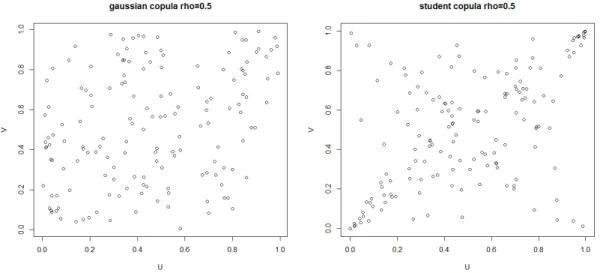
Figure 1: Graph of a joint distribution of copula
Proof. Recall that|a−b|= 2 max(a, b)−(a+b). Using this relation in (14), it’s comes thatf or all h, x∈Rd
M(h) = E(2 max[Z(x+h), Z(x)]−Z(x+h)−Z(x))
2 . (15)
Since E(.) is a linear application, the relation (15) gives
M(h) = E(2 max[Z(x+h), Z(x)])−E(Z(x+h))−E(Z(x))
2 .
Thus,
M(h) =E(max[Z(x+h), Z(x)])−µ. (16) Furthermore,
P(max[Z(x+h), Z(x)]≤z) =P(Z(x+h)≤z, Z(x)≤z),
which is equivalent to:
P(max[Z(x+h), Z(x)]≤z) =Ch(P(Z(x+h)≤z), P(Z(x)≤z)) Thus,
P(max[Z(x+h), Z(x)]≤z) =Ch(FZ(z), FZ(z)), so,
E(max[Z(x+h), Z(x)]) = Z 1
0
FZ−1(u)dCh(u, u).
Substituting this expression in the equation (16) and taking into account thatz=FZ−1(u), we obtain the result:
M(h) = Z 1
0
3.2. Modeling the covariogram via copulas
The variogram allows to measure the linear dependence between the random variables of a field. For two given sites, the associated variogram is given by
ϑ(si, sj) =V ar(Z(si)−Z(sj)) =V ar(Z(si)) +V ar(Z(sj))−2ˆc(si, sj). (17)
These tools do not take into account the extreme data observed in the different observation sites. However, the copula function makes it possible to model the extreme data and to detect any nonlinear link between different observation sites. So, it is necessary to express the variogram and the covariogram via the copula to allow the model to take into account the spatial structure even in case of extremes data. The model could also be able to detect the presence of some nonlinear dependence.
Theorem 2. Let Z ={Z(s1), . . . , Z(sn)} be a stochastic process with variogram given by (14). Then, the covariogramˆc(si, sj) and the copula function are linked by the relation.
ϑ(si, sj) =σ2Z(si) +σ2Z(sj)−2ˆc(si, sj) (18)
where
ˆ
c(si, sj) = Z 1
0
Z 1
0
FZ−1(u)FZ−1(v)c(u, v)dudv−mimj.
The quantity mi being the mean of Z(si); c(u, v) the copula density function attached to
Z(si) andZ(sj).
Proof. Letui =F(Z(si)) =FZ(si). It’s follow that:
zi =FZ−1(ui) =⇒dui =fZ(zi)dzi,
wherefZ(si) is the density function of the variableZ(si). So, it comes that
dzidzj =
1
fZ(zi)fZ(zj)
duiduj.
Similarly, according to Sklar’s theorem [10], it follow that, for all couple of sites (si, sj)∈S2
H(si, sj) =C(FZ(si), FZ(sj)). Moreover,
c(u, v) = f
H1−1(u), Hn−1(un)
f1
F1−1(u1)
×...×Fn
Fn−1(un)
. (19) The relation between the joint density function h(si, sj) and the joint density function of the copulac(u, v) is given by:
Using these expressions in the covariogram expression, it follows that
ˆ
c(si, sj) = Z 1
0
Z 1
0
FZ−1(u)FZ−1(v)c(u, v)dudv−mimj.
By using the last relation in the variogram expression, it follows that
ϑ(si, sj) =σZ2(si) +σZ2(sj)−2 Z 1
0
Z 1
0
FZ−1(u)FZ−1(v)c(u, v)dudv−2mimj.
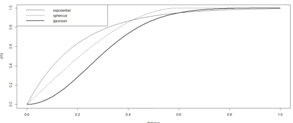
The following figure provide a representation of some theoretical variogram
Figure 2: Graph of some theoretical variograms
3.3. Modeling the correlogram via copulas
The correlogram measures the spatial dependence between two sites si and sj for all i and j. The following result gives a relation between the correlogram and the copula function.
Theorem 3. LetZ ={Z(si), . . . , Z(sj)}be a stochastic process on a geostatistical domain S. For two sitessi, sj ∈S, the correlogram is given, via the associated copula by
ρ(si, sj) = Z 1
0
Z 1
0
FZ−1(u)
σZ(si)
FZ−1(v)
σZ(sj)
c(u, v)dudv− mi
σZ(si)
mj
σZ(sj)
; (20)
where mi denotes the mean of Z(si), c(u, v) = ∂
2C(u,v)
Proof. By definition, the correlogram of a random field in two observation sites is given by:
ρ(si, sj) = ˆ
c(si, sj)
σZ(si)σZ(sj)
= 1
σZ(si)σZ(sj)
×cˆ(si, sj).
Using the result of precedent theorem (theorem 3), we get (20).
3.4. Stationnary framework for covariance modeling
In spatial context, the stationarity describes in a way, a form of spatial homogeneity of regionalization. From a mathematical point of view, stationarity hypothesies consists in assuming that the probabilistic properties of a set of values do not depend on the absolute position of the associated sites, but only on their separation.
Under the assumption of the second order stationarity of the random field Z(.), the mean function deviates a constant and the covariance depends only on the distance sepa-rating the sites. So,
E(Z(si)) =µ ∀i= 1, n and cˆ(si, sj) = ˆc(si−sj) = ˆc(hij).
Previous relationships can be written differently. The following result gives a rela-tionship between the covariogram and the copula function in second-order stationarity case.
Corollary 1. In a second order stationarity framework the covariogram is given by ˆ
c(si, sj) = ˆc(hij) = Z 1
0
Z 1
0
FZ−1(u)FZ−1(v)chij(u, v)dudv−µ
2, (21)
where hij =|si−sj|and chij(u, v) the jointed copula density function of the two localized
variables at two remote sites of hij.
Proof. Under the assumption of two order stationarity, the result of theorem (Theorem 3) gives the relation (21).
Similarly, under the assumption of second-order stationaity, the correlogram and the variogram are expressed as a function af the copula by the relation,
Proposition 2. Assuming thathij =si−sj is the average distance and using the relation (21), then, the correlogram is such as
ρ(hij) = Z 1
0
Z 1
0
FZ−1(u)FZ−1(v) ˆ
c(0Rd)
chij(u, v)dudv−
µ2
ˆ
c(0Rd)
. (22)
and
ϑ(hij) = 2
ˆ
c(0Rd) +µ2−
Z 1
0
Z 1
0
FZ−1(u)FZ−1(v)chij(u, v)dudv
Proof. Under the hypothesis of two order stationary and using the relation (21), the result of theorem (Theorem 3) gives the result (22) and (23).
Proposition 3. The relationship between the variogram and the covariogram is such than,
ˆ
c(hij) = ˆc(0Rd)−
1 2ϑ(hij).
Proof. Let us consider the relations (21) and (23). It is known that:
ˆ
c(si, sj) = ˆc(hij) = Z 1
0
Z 1
0
FZ−1(u)FZ−1(v)chij(u, v)dudv−µ
2,
and
ϑ(hij) = 2
ˆ
c(0Rd) +µ2−
Z 1
0
Z 1
0
FZ−1(u)FZ−1(v)chij(u, v)dudv
.
Adding the two relations above, we get:
2ˆc(hij) +ϑ(hij) = 2ˆc(0Rd).
So
ˆ
c(hij) = ˆc(0Rd)−
1 2ϑ(hij).
3.5. Covariogram in Stationnary intrinsic framework
Consider an intrinsic random fieldZ(.) without drift, that is, the average of the incre-ments is zero and the variance of the increincre-ments is the variogram. The intrinsic hypothesis is written:
E[Z(x+h)−Z(x)] = 0,
and
V ar[Z(x+h)−Z(x)] =E[Z(x+h)−Z(x)]2 = 2γ(h). (24) By integrating the intrinsic hypothesis, we obtain the following result.
Theorem 4. Let Z(.) An intrinsic random field without drift. It follows that the covari-ance is such that
ˆ
c(si, sj) = ˆc(hij) = Z 1
0
Z 1
0
FZ−1(u)FZ−1(v)chij(u, v)dudv−µ
2, (25)
while the correlogram is:
ρ(hij) = Z 1
0
Z 1
0
FZ−1(u)FZ−1(v) ˆ
c(0Rd)
chij(u, v)dudv−
µ2
ˆ
c(0Rd)
And the variogram
ϑ(hij) = 2
ˆ
c(0Rd) +µ2−
Z 1 0
Z 1 0
FZ−1(u)FZ−1(v)chij(u, v)dudv
.
Where µdenote the mean, cˆ(0Rd) the variance and chij(u, v) the density copula function.
Proof. By considering again the relation (24) we obtain:
γ(h) = 1 2E
[Z(x+h)−Z(x)]2 . (26)
Now, it comes that
E[Z(x+h)−Z(x)]2 =E([Z(x+h)]2)−2E(Z(x+h)Z(x)) +E([Z(x)]2).
So, by taking into account the density of the copula,
E
[Z(x+h)−Z(x)]2 = ˆc(0Rd) +µ2−2
Z 1
0
Z 1
0
FZ−1(u)FZ−1(v)chij(u, v)dudv+ ˆc(0Rd) +µ 2.
Furthermore, we have,
E
[Z(x+h)−Z(x)]2 = 2ˆc(0Rd) + 2µ2+−2
Z 1
0
Z 1
0
FZ−1(u)FZ−1(v)chij(u, v)dudv.
Using this last relation in the equation (26), we get finaly,
ϑ(h) = 2
ˆ
c(0Rd) +µ2−
Z 1
0
Z 1
0
FZ−1(u)FZ−1(v)chij(u, v)dudv
. (27)
The variogram expression is similar in the intrinsic and second-order case, we deduce that the covariance and correlogram expressions remain unchanged.
Remark 1. The variogram is related to the covariogram by the relation: ˆ
c(si, sj) = ˆc(hij) = Z 1
0
Z 1
0
FZ−1(u)FZ−1(v)chij(u, v)dudv−µ
2. (28)
and
ϑ(hij) = 2
ˆ
c(0Rd) +µ2−
Z 1
0
Z 1
0
FZ−1(u)FZ−1(v)chij(u, v)dudv
. (29)
Adding the two relations above, we get finaly,
2ˆc(hij) +ϑ(hij) = 2ˆc(0Rd)
and
ˆ
c(hij) = ˆc(0Rd)−
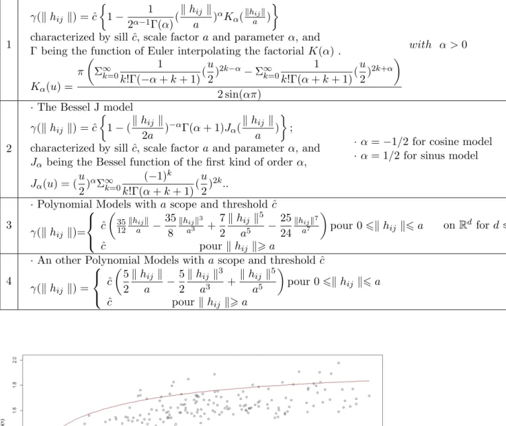
3.6. Mains families of models of variograms
In this section we summary some of the most usefull models of variagrams in spatial modeling
a) Families with bearing or transition models
Families or Modeles of variograms Parameter
1
·Pure nugget effect model
γ(hij) =
0 fori=j
ˆ
c ∀i6=j
·Meaning: reflects an absence of spatial structuring, due at the presence of an undetectable micro-structure experimentally.
2
·Spherical model of parameter rangeaand sill ˆc(valid inRd,d63)
γ(khij k) = (
ˆ
c(7khijk2
a2 −
35 4
khijk3
a3 +
7 2
khijk5
a5 −
3 4
khijk7
a7 ) pour 06khij k6a
ˆ
c pour khij k>a
· Meaning: the presence of an undetectable micro-structure experimentally.
a
3
Gaussian model of parameter a and sill ˆc γ(khij k) = ˆc(1−exp(−
khij k2
a2 ))
·Meaning: the sill is reached asymptotically and the practical range can be taken equal toa√3
a√3
b) Bessel and Polynomial models of variogram
1
·Bessel modified model
γ(khij k) = ˆc
1− 1
2α−1Γ(α)( khij k
a )
αK α(
khijk
a )
characterized by sill ˆc, scale factoraand parameterα, and Γ being the function of Euler interpolating the factorialK(α) .
Kα(u) =
π
Σ∞k=0 1
k!Γ(−α+k+ 1)(
u
2)
2k−α−Σ∞
k=0
1
k!Γ(α+k+ 1)(
u
2)
2k+α
2 sin(απ)
with α >0
2
·The Bessel J model
γ(khij k) = ˆc
1−(khij k 2a )
−αΓ(α+ 1)J α(
khij k
a )
; characterized by sill ˆc, scale factoraand parameterα, and
Jα being the Bessel function of the first kind of order α,
Jα(u) = (
u
2) αΣ∞
k=0
(−1)k
k!Γ(α+k+ 1)(
u
2)
2k..
·α=−1/2 for cosine model
·α= 1/2 for sinus model
3
·Polynomial Models witha scope and threshold ˆc
γ(khij k)= ˆ c 35 12
khijk
a − 35
8 khijk3
a3 +
7 2
khij k5
a5 −
25 24
khijk7
a7
pour 06khij k6a ˆ
c pour khij k>a
onRd ford63
4
·An other Polynomial Models withascope and threshold ˆc
γ(khij k) = ˆ c 5 2
khij k
a −
5 2
khij k3
a3 +
khij k5
a5
pour 06khij k6a ˆ
c pour khij k>a
4. Conclusion
The results of the study provides important characterizations of the variogram, the correlogram in a copula framework. Especially, they show on one hand that these tools are limited when data includes extremes values, in an other hand, that they have a copulawise extension, allowing the copula to model the data in the spatial context. Moreover, the study provides tools to analyze data and perform a comparative study with existing tools.
References
[1] Barro, D. (2009). Conditional Dependence of Trivariate Generalized Pareto Dis-tributions, Asian Journal of Mathematics & Statistics Vol. 2 No.2, 20-32. DOI: ajms.2009.20.32
[2] Barro, D. (2012). Geostatistical Analysis with Conditional Extremal Copulas, Inter-national Journal of Statistics and Probability; Vol. 1 No.2, 2012. ISSN 1927-7032 E-ISSN 1927-7040
[3] Beirlant J., Goegebeur Y, Segers J. and Teugels,J. (2005). Statistics of Extremes: theory and application, Wiley, Chichester, England.
[4] Bondar, I., McLaughlin, K., & Israelsson, H. (2005). Improved Event Location Un-certainty Estimates, 27th Seismic Research Review, 299-307
[5] Bordossy, A. (2006). Copula based geostatistical models for groundwater quality pa-rameters. Water Resources Research 42.
[6] Cooley D. Poncet P. and P. Naveau (2006). Variograms for max-stable random .elds. In Dependence in 8 Probability and Statistics. Lecture Notes in Statistics 187 373.390. Springer, New York
[7] Dossou-Gbete S., B., Som´e and Barro, D. (2009). Modelling the Dependence of Para-metric Bivariate Extreme Value Copulas, Asian Journal of Mathematics & Statistics, Vol 2, Issue3, 41-54 DOI: .3923/ajms.2009.41.54
[8] Kazianka, H.(2009). Spatial modeling and interpolation using copulas. PhD thesis, University of Klagenfurt. Ribatet (2011)- Statistical Modelling of Spatial Extremes A. C. Davison, S. A. Padoan and M. Ribatet October 3, 2011
[9] Nelsen, R.B. (1999). An Introduction to copulas. Lectures notes in Statistics 139, Springer-Verlag Joe H., 1997, Multivariate Models and Dependence Concepts. Mono-graphs on Statistics and Applied Probabilty 73, Chapman and Hall, London. ISBN 978-0-412-7331
[11] Sklar, A.(1973). Random variables, joint distribution functions, and copu-las.Kybernetika, 9(6),449-460.9
[12] Schmitz, V. (2003). Copulas and Stochastic Processes, Aachen University, PhD dis-sertation
[13] M.Frechet Sur la loi de probabilit ˜A c de l’ ˜A ccart maximum. Annales de la soci ˜A ct ˜A c Polonaise de Math ˜A cmatiques,6.(1927).93-116.
[14] D. Barro Contribution ˜A la mod ˜A clisation statistique des valeurs extr ˜Aames mul-tivari ˜A ces. Th ˜A¨se de l’Universit ˜A cde Ouagadougou. D ˜A ccembre (2010)
[15] P.J.Diggle & P.J.Ribeiro Jr. Model-based Geostatistics. Springer Series in Statistics, Springer Science and Business Media, LLC, Springer. New York. (2007).
[16] C. Dombry Th ˜A corie spatiale des extr ˜Aames et propri ˜A ct ˜A cs des processus max-stables. Document de synth ˜A¨se en vue de l’habilitation ˜A diriger des recherches, Universit ˜A c de Poitiers, UFR Sciences Fondamentales et Appliqu ˜A ces. Novembre (2012).
[17] R.A. Fisher & L.H.C. Tippett. Limiting Forms of the Frequency of the Largest or Smallest Member of a Sample. Proceedings of the Cambridge Philosophical Society, 24.(1928). 180-190.
[18] C. Fonseca, L. Pereira, H. Ferreira & A.P. Martins. Generalized Madogram and Pair-wise Dependence of Maxima over two Regions of a Random Fiel. arXiv: 1104.2637v2 [math.ST] 24 Jan 2012. (2012).
[19] A.L. Foug ˜A¨res & P. Soulier. Limit Conditional Distributions for Bivariate Vectors with Polar Representation. Stochastic Models, 26(1). (2010). 54-77.
[20] M. Fr ˜A cchet. Sur la loi de probabilit ˜A c de l’ ˜A ccart maximum. Annales de la soci ˜A ct ˜A c Polonaise de Math ˜A cmatiques, 6. (1927). 93-116. C. Gaet
[21] Beirlant, J., Goegebeur, Y., Segers, J., and Teugels, J. (2005).Statistics of Extremes: theory and application -Wiley, Chichester, England.
[22] Coles, S. (2001). An introduction to statistical modeling of extreme values- Springer-Verlag (London), 2001.
[23] Degen M. (2006). On Multivariate Generalised Pareto Distributions and High Risk Scenarios - thesis, Department of Mathematics, ETH Z¨urich.
[24] D. Barro (2009) Conditional Dependence of Trivariate Generalized Pareto Distribu-tions.Asian Journal of Mathematics & Statistics Year: 2009|Volume: 2|Issue: 2 |
[25] Diakarya Barro, Moumouni Diallo, and Remi Guillaume Bagr ˜A c, “Spatial Tail De-pendence and Survival Stability in a Class of Archimedean Copulas,” Inter. J. of Mathematics and Mathematical Sciences, vol. 2016, Article ID 8927248, 8 pages, 2016. doi:10.1155/2016/8927248
[26] Ferreira, H. and Ferreira,M. (2012) Fragility Index of block tailed vectors. ScienceDi-rect. ELsevier vol. 142 (7), 1837–1848 http ://dx.doi.org/10.1016/j.bbr.2011.03.031 [27] Foug ˜A¨res, A., L (1996). Estimation non param ˜Actrique de densit ˜Acs unimodales
et de fonctions de d ˜Acpendance- th ˜A¨ses doctorat de l’Universit ˜A c Paul Sabatier de Toulouse.
[28] Husler, J., Reiss, R.-D.(1989).Extreme value theory - Proceedings of a conference held in Oberwolfach, Dec. 6-12,1987. Springer, Berlin etc. Lenz, H.
[29] Joe, H. (1997). Multivariate Models and Dependence Concepts - Monographs on Statistics and Applied Probabilty 73, Chapman and Hall, London.
[30] Kotz, S., Nadarajah, S. (2000). Extreme Value Distributions, Theory and Applica-tions - Imperial College Press - [48] S. Lang , Linear Algebra
[31] Michel, R.(2006).Simulation and Estimation in Multivariate Generalized Pareto Dis-tributions- Dissertation, Fakult¨at f¨ur Mathematik, Universit¨at W¨urzburg, W¨urzburg. [32] Nelsen, R.B. (1999). An Introduction to copulas- Lectures notes in Statistics 139,
Springer-Verlag
[33] Resnick, S.I. (1987). Extreme Values, Regular Variation and Point Processes-Springer-Verlag.
[34] Schmitz, V. (2003). Copulas and Stochastic Processes, Aachen University, PhD dis-sertation