Rajan Transform and its Uses in Pattern Recognition
Ekambaram Naidu Mandalapu
Professor, TRR College of Engineering, Hyderabad, India Research Scholar of the University of Mysore
E-mail: [email protected]
Rajan E. G. Professor and Dean
JB Institute of Engineering & Technology, Hyderabad President, Pentagram Research Foundation
An Undertaking of Pentagram Research Centre (P) Limited, India E-mail: [email protected]
Keywords:transform, pattern classification, image processing, permutation invariant systems
Received:June 13, 2006
This transform was introduced in the year 1997 by Rajan [2], [4] on the lines of Hadamard Transform. This paper presents, in addition to its formulation, the algebraic properties of the transform and its uses in pattern recognition. Rajan Transform (RT) is a coding morphism by which a number sequence (integer, rational, real or complex) of length equal to any power of two is transformed into a highly correlated number sequence of the same length. It is a homomorphism that maps a set consisting of a number sequence, its graphical inverse and their cyclic and dyadic permutations, to a set consisting of a unique number sequence ensuring the invariance property under such permutations. This invariance property is also true for the permutation class of the dual sequence of the number sequence under consideration. A number sequence and its dual are like an object and its mirror image. For example, the four point sequences x(n) = 3, 1, 3, 3 and y(n) = 2, 4, 2, 2 are duals to each other. Observe that the sum of each sequence is 10 and one sequence could be obtained from the other by subtracting the elements of the other sequence from 5, which is half of its sum. Since RT of a number sequence is an organized number sequence with a high degree of correlation, it is suitable for effective data compression. This paper describes in detail the techniques of using RT for pattern recognition purposes. For example, pattern recognition operations like extracting lines, curves, isolated points and points of intersection of lines from a digital gray or colour image could be carried out using RT based fast algorithms.
Povzetek: Prispevek opisuje Rajanovo transformacijo in njeno uporabo v prepoznavanju vzorcev.
1 Introduction
Pattern recognition is essentially a classification process. Set-theoretically, it is partitioning of domain set by a rule. One can also visualize pattern recognition as a homomorphic map connecting domain and range sets, while isomorphic maps are used for the purpose of analysis. Mostly, mathematical transforms are associated with inverses and hence they are isomorphic in nature. For example, Discrete Fourier Transform is defined as an Analysis-Synthesis pair like many other transforms. It is reasonable to raise a question here whether at all it is possible to develop a homomorphic transform, which would advocate operations related to pattern recognition. It is after a prolonged research and study of related techniques like Permutation Invariant Systems and Number Theory, that Professor Rajan and his research team introduced in the year 1997 a novel algorithm for classification purposes, which they called as Rapid Transform. Subsequent research on the algebraic properties of this transform has exposed its richness and recently it was renamed as Rajan Transform (RT). The
purpose of this paper is to report the research carried out till date on the algebraic properties of RT and its role in developing high- speed pattern recognition algorithms like contour detection, thinning, corners detection, lines detection, curves detection, and detection of isolated points in a given grey or colour image. Some algebraic properties like Regenerative Property of RT are found to have potential applications related to Cryptography.
2 Rajan Transform
Rajan Transform is essentially a fast algorithm developed on the lines of Decimation-In-Frequency (DIF) Fast Fourier Transform algorithm, but it is different from the DIF-FFT algorithm. Given a number sequence x(n) of length N, which is a power of 2, first it is divided into the first half and the second half each consisting of (N/2) points so that the following hold good.
Now each (N/2)–point segment is further divided into two halves each consisting of (N/4) points so that the following hold good.
g1(k) = g(j) + g(j + (N/4)) ; 0k(N/4) ; 0j(N/4)
g2(k) = |g(j) - g(j - (N/4))| ; 0k(N/4); (N/4)j(N/2)
h1(k) = h(j) + h(j + (N/4)) ; 0k(N/4); 0j(N/4)
h2(k) = |h(j) - h(j - (N/4))| ; 0k(N/4); (N/4)j(N/2)
This process is continued till no more division is possible. The total number of stages thus turns out to be log2N. Let us denote the sum and difference operators
respectively as + and ~.
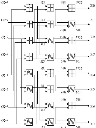
Then the signal flow graph for the Rajan Transform of a number sequence of length 8 would be of the form shown in figure 2.1.
If x(n) is a number sequence of length N = 2k; K>0,
then its Rajan Transform is denoted as X(k). RT is applicable to any number sequence and it induces an isomorphism in a class of sequences, that is, it maps a domain set consisting of the cyclic and dyadic permutations of a sequence on to a range set consisting of sequences of the form X(k)E(r) where x(k) denotes the permutation invariant RT and E(r) an encryption code corresponding to an element in the domain set. This map is a one-to-one and on to correspondence and an inverse map also exists. Hence it is viewed as a transform. Consider a sequence x(n) = 3, 8, 5, 6, 0, 2, 9, 6. Then X(k) = 39, 5, 13, 9, 13, 1, 7, 5. The signal flow graph for
Figure 2.1: Signal flow diagram of one-dimensional 8-point RT.
this transform together with the encryption key (number 0 or 1 inside the brackets) is given in figure 2.1.
Observe from the diagram that E(r) is a union of three sequences E1(r) = 0, 0, 0, 0, 1, 1, 0, 0 , E2(r) = 0, 0,
0, 0, 0, 0, 0, 1 and E3(r) = 0, 0, 0, 1, 0, 1, 0, 0. That is,
E(r) = E1(r)E2(r)E3(r). Now, the sequence X(k)E(r) = 39,
5, 13, 9, 13, 1, 7, 5, 0, 0, 0, 0, 1, 1, 0, 0, 0, 0, 0, 0, 0, 0, 0, 1, 0, 0, 0, 1, 0, 1, 0, 0 is the RT of the input sequence x(n) = 3, 8, 5, 6, 0, 2, 9, 6. In general, the first point in a RT is called ‘Cumulative point Index’ (CPI).
A closed form expression for RT is described below. RT is applicable to sequences consisting of both positive as well as negative numbers. The forward transform can be obtained by operating the input sequence using a matrix operator called Rmatrix, recursively by dividing
input sequence as well as by partitioning the Rmatrix in
the following manner.
….2.1
X is the column matrix containing input sequence of length N. IN/2is the identity matrix of size N/2, that is,
half the size of the input sequence matrix XNX1. Basic
identity matrix I1=1; and ek is the encryption function
with k as encryption value which is defined as ek= (-1)ksuch that
k = 1; for x(i + N/2) < x(i) ; 0≤i≤N/2 ... 2.2 = 0; otherwise,
and x(i) is the ithelement of matrix X
NX1. Now divide the
matrix ANX1 into two column matrices, namely A00and
A01of size N/2 and treating these matrices as two input
sequences, compute the two new A10and A11 matrices by
using the operator RN/2for both the sequences. Note that
size of the R matrices used is one half of the original RN
matrix. Continue the above procedure iteratively till the size of the sub matrices is reduced to two. So, we have N = 2n-p, for pthiteration stage, with p = 1, 2,…, n. All the
encryption binary values, that is, k values thus generated during the process of computation per iteration are to be associated with the final spectrum, to recover the original sequence through inverse transformation technique. Note that this closed form expression precisely defines the algorithm stated in the beginning of this section.
3 Inverse Rajan Transform
Retrieval of the information or the signal x(n) can be done by Inverse Rajan Transform (IRT) [2], [4]. The basic requirements for the IRT computation are the RT coefficients associated with the encryption values (k values) that are generated by encryption function while computing forward RT.
The strategy adopted here is to retrace the forward transform signal flow graph. It was observed that the point-wise addition of a constant value, say K to the sample sequence x(n) while computing forward RT, changes only the DC component X0, that is, the CPI to
computed RT, and the remaining spectral values remain the same of the original spectrum. For example, the RT spectrum X(k) of the sequence x(n) = 3, 8, 5, 6, 0, 2, 9, 6 is 39, 5, 13, 9, 13, 1, 7, 5. Now let us build a new sequence x1(n) = 4, 9, 6, 7, 1, 3, 10, 7 by adding K=1 to
the sequence x(n) = 3, 8, 5, 6, 0, 2, 9, 6. The RT spectrum of the new sequence is X1(k) = 47, 5, 13, 9, 13,
1, 7, 5.
Now, in order to work with sequences containing negative sample values, we proceed as usual in the case of forward transform. But, the inverse transform is calculated just by adding a constant value N(2M-1) to the
CPI value of the spectrum. M is the bit length required to represent the maximum quantization level of the samples and N is the length of the sequence. This constant factor K = (2M-1) is chosen such that all the maximum possible
negative values of the sequence x(n) are level shifted to 0 or above. This DC shift is required, because we hide the sign of the negative values that are generated while computing the forward RT. As mentioned earlier, RT induces an isomorphism between the domain set consisting of the inverse, cyclic, dyadic and dual class permutations of a sequence on to a range set consisting of sequences of the form X(k)E(r) where X(k) denotes the permutation invariant RT and E(r) an encryption code corresponding to an element in the domain set. This map is a one-to-one and on-to correspondence and an inverse map also exists. Thus RT is viewed as a transform. Now we provide a technique for obtaining the inverse of Rajan Transform.
Inverse Rajan transform (IRT) is a recursive algorithm and it transforms a RT code X(k)E(r) of length N(1+m) where N = 2mand m is the number of stages of
computation, into one of its original sequences belonging to its permutation class depending on the encryption code E(r). The computation of IRT is carried out in the following manner. First the input sequence is divided into segments each consisting of two points so that either
g(2j+1) = (X(2k)+X(2k+1))/2
g(2j) = max (X(2k), X(2k+1))-g(2j+1)
if E1(2r)= 0 and E1(2r+1) = 0;
0j<N; 0kN; 0rN, or
g(2j) = (X(2k)+X(2k+1))/2
g(2j+1) = max (X(2k), X(2k+1) - g(2j) if E1(2r) = 1 or E1(2r+1) = 1;
0jN; 0kN; 0rN.
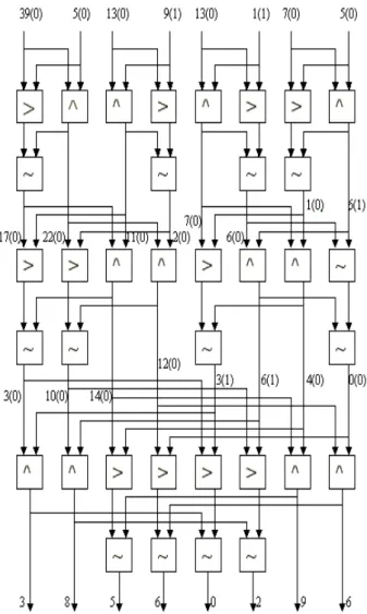
The resulting sequence is divided into segments each consisting of four points. Each 4-point segment is synthesized as per the above procedure. The resulting sequence is further divided into segments each consisting of eight points and the same procedure is carried out. This process is continued till no more division is possible. Consider X(k) = 39, 5, 13, 9, 13, 1, 7, 5. Then its IRT is x(n) = 3, 8, 5, 6, 0, 2, 9, 6. The inverse x(n) is obtained from the given X(k)E(r) as shown in figure 3.1.
The symbols ^ > and ~ respectively denote the operators average of two, maximum of two and difference of two. Note that IRT will work only in the presence of encryption sequence E(r) and for every member of the permutation class there would be a unique
encryption sequence. Study of the class of encryption sequences corresponding input sequences itself is a field of active research.
Figure 3.1: Signal flow diagram of IRT of a spectral sequence.
As already outlined that RT hides negative signs and so it is important to add N(2M-1) to X(0) in order to get back
the original sequence. Let XNX1be the column matrix of
the RT coefficients of length N, and the associated encryption values generated per iteration are orderly arranged in the form of column matrices E1, E2, …, En-1,
of length N/2, where n = log2N . For N = 8, we have E1
and E2
, two encryption matrices of size 4X1 with binary
encryption values as elements. Here XNX1 is the RT
coefficient matrix. RNX1is the intermediate matrix. ANX1
is the matrix with the elements positioned in their appropriate positions using the encryption matrix Er
corresponding to the current iteration. Ēr is the matrix obtained by element wise complementing the Ermatrix,
where r = n-1, n-2, …, 1.
computation. Each encryption matrix is to be partitioned as per the requirement.
The closed form expression shown as equation 3.1 represents the Inverse Rajan Transform. For example, let us consider a sequence x(n) which has a maximum
sample value of –15. The RT of this sequence is X(k). ……3.1
Now one can assume the value of M to be 4 so that the maximum negative sample value in the sequence is –15. Addition of +15 to each sample value in an 8-point input sequence x(n) will lead to the sequence x1(n) = x(0)+15,
x(1)+15, … , x(7)+15, which is level shifted to 0 and above. Now the spectrum of this level shifted sequence x1(n) would be X1(k) = X1(0), X1(1), … , X1(7), where
X1(0) = X(0)+120, X1(1) = X(1), … , X1(7) = X(7).
A specific example would make things easy. Let us consider a sequence x(n) = 3, 8, 5, 6, 0, 2, 9, 6 and its RT, X(k) = 39, 5, 13, 9, 13, 1, 7, 5. Now addition of 15 to each sample point in x(n) would yield a sequence x1(n) =
18, 23, 20, 21, 15, 17, 24, 21 and its RT would be X1(k)
= 159, 5, 13, 9, 13, 1, 7, 5. Observe that X1(0) = X(0) +
120 = 39 + 120 = 159. As outlined earlier, one can add N(2M-1) to X(0) of a spectral sequence and compute the
IRT as usual. Then it is important to subtract 2M-1 from
every sample point so as to obtain the actual sample domain sequence. Let us take the case of X(k) = 39, 5, 13, 9, 13, 1, 7, 5. Now let us add 120 only to X(0) so that the spectral sequence becomes 159, 5, 13, 9, 13, 1, 7, 5. The IRT of this sequence is 18, 23, 20, 21, 15, 17, 24, 21. By subtracting 15 from each sample value we obtain the actual sequence 3, 8, 5, 6, 0, 2, 9, 6.
4 Algebraic Properties of Rajan
Transform
RT has interesting algebraic properties like permutation invariance, scalar property and linear pair forming property. All such properties are explained in detail in the following.
4.1 Cyclic shift invariance property
Let us consider the same sequence x(n) = 3, 8, 5, 6, 0, 2, 9, 6. Using this sequence one can generate seven more cyclic shifted versions such as xc1(n) = 6, 3, 8, 5, 6, 0, 2,
9 , xc2(n) = 9, 6, 3, 8, 5, 6, 0, 2 , xc3(n) = 2, 9, 6, 3, 8, 5, 6,
0 , xc4(n) = 0, 2, 9, 6, 3, 8, 5, 6 , xc5(n) = 6, 0, 2, 9, 6, 3, 8,
5 , xc6(n) = 5, 6, 0, 2, 9, 6, 3, 8 and xc7(n) = 8, 5, 6, 0, 2,
9, 6, 3. It is obvious that the cyclic shifted version of xc7(n) is x(n) itself. One can easily verify that all these
eight sequences have the same X(k), that is, the sequence 39, 5, 13, 9, 13, 1, 7, 5 but different E(r).
4.2 Graphical inverse invariance property
The sequence x(n) = 3, 8, 5, 6, 0, 2, 9, 6 has the graphical inverse x-1(n) = 6, 9, 2, 0, 6, 5, 8, 3. Using this sequence one can generate seven more cyclic shifted versions such as xc1-1(n) = 3, 6, 9, 2, 0, 6, 5, 8 , xc2-1(n) = 8, 3, 6, 9, 2,
0, 6, 5 , xc3-1(n) = 5, 8, 3, 6, 9, 2, 0, 6 , xc4-1(n) = 6, 5, 8, 3,
6, 9, 2, 0 , xc5-1(n) = 0, 6, 5, 8, 3, 6, 9, 2 , xc6-1(n) = 2, 0,
6, 5, 8, 3, 6, 9 and xc7-1(n) = 9, 2, 0, 6, 5, 8, 3, 6. It is
obvious that the cyclic shifted version of xc7-1(n) is x-1(n)
itself. One can easily verify that all these eight sequences have the same X(k), that is, the sequence 39, 5, 13, 9, 13, 1, 7, 5 but different E(r)
4.3 Dyadic shift invariance property
The term ‘dyad’ refers to a group of two, and the term ‘dyadic shift’ to the operation of transposition of two blocks of elements in a sequence. For instance, let us take x(n) = 3, 8, 5, 6, 0, 2, 9, 6 and transpose its first half with the second half. The resulting sequence Td(2)[x(n)] =
0, 2, 9, 6, 3, 8, 5, 6 is the 2-block dyadic shifted version of x (n). The symbol Td(2) denotes the 2-block dyadic
shift operator. In the same manner, we obtain Td(4)[Td(2)[x(n)]] = 9, 6, 0, 2, 5, 6, 3, 8 and
Td(8)[Td(4)[Td(2)[x(n)]]]=6, 9, 2, 0, 6, 5, 8, 3. One can
easily verify that all these dyadic shifted sequences have the same X(k), that is, the sequence 39, 5, 13, 9, 13, 7, 5 but different E(r). There is yet another way of dyadic shifting the input sequence x(n) to Td(2)[Td(4)[Td(8)[x(n)]]].
Let us take x(n) = 3, 8, 5, 6, 0, 2, 9, 6 and obtain the following dyadic shifts: Td(8)[x(n)] = 8, 3, 6, 5, 2, 0, 6, 9 ,
Td(4)[Td(8)[x(n)]] = 6, 5, 8, 3, 6, 9, 2, 0 and
Td(2)[Td(4)[Td(8)[x(n)]]] = 6, 9, 2, 0, 6, 5, 8, 3. Note that
Td(2)[Td(4)[Td(8)[x(n)]]] = Td(8)[Td(4)[Td(2)[x(n)]]]. One can
easily verify from the above that other than Td(4)[Td(2)[x(n)]] and Td(8)[x(n)], all other dyadically
permuted sequences fall under the category of the cyclic permutation class of x(n) and x-1(n). This amounts to saying that the cyclic permutation class of x(n) has eight non-repeating independent sequences, that of x-1(n) has
eight non-repeating independent sequences and the dyadic permutation classes of x(n) has two non-repeating independent sequences. To conclude, all these 18 sequences could be seen to have the same X(k). Each of these 18 sequences has an independent encryption key E(r).
4.4 Dual class invariance
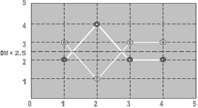
Given a sequence x(n), one can construct another sequence y(n) consisting of at least one number which is not present in x(n) such that X(k) = Y(k). In such a case, y(n) is called the dual of x(n). Consider two sequences x(n) = 2, 4, 2, 2 and y(n) = 3, 1, 3, 3. Then X(k) = Y(k) = 10, 2, 2, 2. Figure 4.4.1 shows the symmetry property of the sequences x(n) and y(n). The term Differential Mean (DM) refers to the mean about which the two sequences are symmetrical to each other.
Figure 4.4.1: Symmetry property of dual sequences (DM=2.5).
The major contribution of this paper is a characterization theorem (theorem 4.4.1) for classifying sequences, which have dual sequences.
Theorem 4.4.1: A sequence of length N=2n is said to
have a dual if and only if its CPI is an even number and is divisible by N/2.
Corollary 4.4.1.1:Theorem 4.4.1 advocates a necessary
condition but not a sufficient condition. This means that all sequences that satisfy theorem 4.4.1 need not form valid dual pairs with other sequence vide definition of dual. For example, let us consider the sequence x(n) = 6, 8, 2, 0. This satisfies theorem 4.4.1. That is its CPI is 16 and the value of CPI/(N/2) is 8. Now its dual is computed as y(n) = 2, 0, 6, 8 , which is not a dual of x(n) as per the definition.
PROPERTIES OF DUAL SEQUENCES
1. If y(n) is a dual of x(n), then x(n) is also called the dual of y(n). Hence the pair <x(n), y(n)> is called ‘dual pair’.
2. Dual of a sequence, say y(n) will necessarily exhibit geometric symmetry together with the original sequence x(n).
3. Each dual pair has a value called ‘Differential Mean’ (DM), which is equal to (|x(i)-y(i)|)/2; 0
i (N-1). It is obvious that the DM could be a real number.
4.5 Regenerative property
As per theorem 4.4.1, an arbitrary sequence x(n) of length N=2nis said to have a dual y(n) if and only if its
CPI is an even number and is divisible by N/2. In other words, x(n) is said to form a dual pair with y(n). It was observed that the sequence |x(0)-y(0)|, |x(1)-y(1)|,
|x(2)-y(2)|, ….., |x(N-2)-y(N-2)|, |x(N-1)-y(N-1)| also satisfies theorem 4.4.1 and is eligible to form a dual pair with yet another sequence. For example let us consider a sequence x(n) = 3, 1, 3, 3. This satisfies theorem 4.4.1 since its CPI is 10 and it is divisible by N/2, that is, 2 yielding the value 5. Now one can obtain the dual sequence y(n) = 2, 4, 2, 2 by subtracting each element of x(n) from 5. Now x(n) and y(n) form a pair and yield their ‘first generation sequence’, say x1(n) = 1, 3, 1, 1 , which is obtained by
finding the point wise difference between the parent sequences x(n) and y(n). One can easily verify that x1(n)
also satisfies theorem 4.4.1 and forms a dual pair with y1(n) = 2, 0, 2, 2. This property is termed here as
‘regenerative property’. Another important observation follows. x1(n) forms a dual pair with y1(n) but this pair
does not produce an offspring sequence as it was done by the pair <x(n), y(n)>.This could be easily verified by the fact that the point wise difference between x1(n) and
y1(n) yields x1(n) only. Hence for brevity we call the
sequences x1(n) and y1(n) as ‘sterile sequences’ and the
pair <x1(n), y1(n)> as a ‘sterile pair’. This property
exhibits the possibility of further research on generative and sterile pairs.
4.6 Scalar property
Let x(n) be a number sequence and be a scalar. Then the RT of x(n) will be X(k), where X(k) is the RT of x(n). For example, let us consider a sequence x(n) = 1, 3, 1, 2 and a scalar of value 2. Now the RT X(k) of x(n) is 7, 3, 1, 1. The RT of x(n) = 2, 6, 2, 4 is 14, 6, 2, 2 which is nothing but X(k).
4.7 Linearity property
In general, RT does not satisfy the linearity property. However, it was observed that for a pair x(n) and y(n) which are number sequences either in the increasing order or in the decreasing order, the linearity property holds. That is, for x(n)+my(n) where and m are scalars and x(n) and y(n) are two number sequences either in the increasing or decreasing order, the RT will be
X(k)+mY(k), where X(k) and Y(k) are respectively the RTs of x(n) and y(n). A characterization theorem is yet to be established for categorizing pairs of sequences which would satisfy linearity property.
4.8 Linear pair forming property
purposes. For instance let us consider two arbitrary sequences x(n) and y(n) given below:
x(n) = 2, 2, 2, 1, 6, 2, 6, 1, 2, 3, 0, 0, 2, 5, 5, 4; y(n) = 4, 5, 3, 1, 0, 1, 4, 6, 6, 8, 0, 0, 7, 9, 0, 5;
Now the RT of x(n) denoted as X1(k) is computed as
X1(k) = 43, 7, 7, 5, 19, 7, 7, 3, 15, 1, 1, 1, 9, 1, 3, 3 and
the RT of y(n) denoted as Y1(k) is computed as Y1(k) =
59, 11, 21, 1, 17, 9, 9, 5, 29, 3, 11, 7, 11, 1, 9, 1. Now, z(n) = x(n) + y(n) is given by the sequence 6, 7, 5, 2, 6, 3, 10, 7, 8, 11, 0, 0, 9, 14, 16, 6, 8, 6, 8, 6, where as X1(k) +
Y1(k) = 102, 18, 28, 6, 36, 16, 16, 8, 34, 4, 12, 8, 20, 2,
12, 4. Note that Z(k) is not equal to X1(k) + Y1(k). Now,
the second order RT spectra of X1(k) and Y1(k) are
respectively computed as X2(k) = 132, 76, 72, 64, 32, 32,
28, 28, 64, 32, 36, 20, 24, 16, 20, 12 and Y2(k) = 204,
128, 76, 56, 80, 68, 48, 44, 72, 20, 32, 20, 36, 32, 16, 12. Let z1(n) be the sequence X1(k) + Y1(k). Then Z1(k) is
the RT of and z1(n) and is computed to be 326, 194, 138,
110, 98, 86, 70, 66, 138, 70, 86, 42, 66, 62, 42, 38. Note that Z1(k) is not equal to X2(k) + Y2(k) = 336, 204, 148,
120, 112, 100, 76, 72, 136, 52, 68, 40, 60, 48, 36, 24. This procedure is repeated for the third order spectra as follows: X3(k) = 688, 128, 128, 64, 304, 96, 96, 64, 240,
0, 32, 32, 144, 32, 32, 32 and Y3(k) = 944, 184, 336, 104,
272, 136, 144, 88, 464, 40, 176, 24, 176, 24, 144, 8 are the RTs of X2(k) and Y2(k) respectively. The RT of
X2(k) + Y2(k) is computed to be 1632, 312, 464, 168,
576, 232, 240, 152, 704, 40, 208, 56, 320, 56, 176, 40 which is nothing but X3(k) + Y3(k). Thus it is clear from
the above example that higher order RT spectra of arbitrary sequences of equal length do form linear pairs, and so the name ‘linear pair forming property’. Linear pair forming property is also called self-organizing property.
5 Pattern Recognition and Processing
using Rajan Transform
5.1 Basic philosophy
Spectral domain image processing advocates the manipulation of spectral components in deciding the conditions for extracting various features in a given image. For example, high pass filtering of frequency spectral components allows the extraction of edges in a digital image, where as, low pass filtering of frequency spectral components causes smoothing of edges. Rajan Transform is basically a fast algorithm which yields spectral components of a signal sequence. Thus it is
reasonable to surmise that one can as well think of using RT for spectral domain processing of digital images and one may proceed on the following lines. The given digital image is scanned by the neighbourhood window, which is shown in figure 5.1.1.
The image pixels corresponding to the cells in the window are labeled as x0, x1, x2, x3, x4, x5, x6 and x7.RT
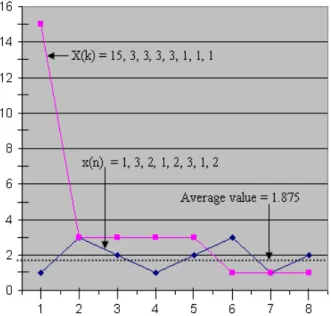
of this sequence is X(k). The CPI is divided by 8, which yields the average value. The number of spectral values in the RT sequence, which are below or above the average value, plays an important role in the processing of an image. Consider a sequence x(n) = 1, 3, 2, 1, 2, 3, 1, 2 and its RT : X(k) = 15, 3, 3, 3, 3, 1, 1, 1.
Figure 5.1.2: Pictorial representation of x(n) and X(k).
With reference to figure 5.1.2, the CPI: X0 is 15 and the
average value is X0 / 8 = 15 / 8 = 1.875. Note that there
are three spectral values less than the average value and three are above the average value, excluding X0. The
spectral components 1, 1 and 1 shown in figure 5.1.2 are less than the average value 1.875. The central pixel value of the image is updated based on such facts.
5.2 Sample algorithms for image processing
and pattern recognition
In what follows, we discuss RT based fast algorithms for certain traditional image processing operations like contouring and thinning and for pattern recognition operations like corners detection, lines detection and curves detection [3].
5.2.1
Contouring algorithm
Otherwise, the window moves to the right. This procedure is continued till the entire image is scanned.
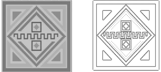
The overall effect is that the boundaries of regions that appear to be uniform are retained and the central pixels are erased. One can always choose the value of T from 3 to 7 depending on the requirement. Figure 5.2.1.1 shows the digital image of a pattern and its contour map obtained the RT based algorithm.
Figure 5.2.1.1: Original image and its contour map.
5.2.2
Thinning algorithm
Thinning is the complementing operation of contouring. The algorithm given for contouring is used in this case also but with the exception that instead of removing the central pixel, the boundary pixels are removed. This operation is otherwise called Onion Peeling. Repeated boundary removal leads to thinned version of the original image. Figure 5.2.2.1 shows the pattern and its thinned version obtained the above RT based thinning algorithm.
Figure 5.2.2.1: Original image and its thinned version.
5.2.3
Corners detection
On every move of the 3X3 window, the RT sequence,
say, G[0],G[1],G[2],G[3],G[4],G[5],G[6],G[7]
corresponding to the sequence of the numbered cell values is checked for the following conditions :
Corners due to pairs of lines subtending an angle of 45or its integral multiples:
(1) The number of RT elements that are less than T must be 4. (2) Alternate RT elements G[0], G[2], G[4], and G[6] should be greater than T.
Corners due to pairs of lines subtending 90 or its integral multiples:
(1) The number of RT elements that are less than T must be 4. (2) The RT elements G[0], G[1], G[4] and G[5] should be greater than T.
The above procedure is repeated till the entire image is scanned. The overall effect is that the resulting image would consist only of corner points. Figure 5.2.3.1 shows the image of the contoured pattern and its processed image consisting of corners only using the above RT based corners detection algorithm.
Figure 5.2.3.1: Contoured pattern and image consisting of corners.
5.2.4
Lines detection
On every move of the 3X3 window, the RT of each boundary values sequence is checked for the following condition:
(1) The number of RT elements that are less than T must be 4. (2) The first four RT elements including the CPI should be greater than T.
In such a case, the central pixel has to be a mid point of a line and so is chosen. The overall effect is that the resulting image would consist only of straight lines. Figure 5.2.4.1 shows the image of the contoured pattern and its processed image consisting of lines only using the above RT based lines detection algorithm.
Figure 5.2.4.1: Contoured pattern and image consisting of lines.
5.2.5
Curves detection
Figure 5.2.5.1: Contoured pattern and image consisting of curves
6 Conclusions
Rajan Transform has been used as a high-speed spectral domain tool to carry out pattern recognition and digital image processing operations. Some of the algorithms meant for pattern recognition using feature extraction have been presented in this paper. Recent investigations show that RT could be one of the best tools that could be used in cryptography. RT based watermarking of text and images and character recognition would yield a repertoire of tools of the future. Efforts are being made to abstract the notion of RT to Symbolic Processing of Signals and Images in the DNA computing paradigm.
7 Acknowledgements
This paper is the result of a fundamental research carried out in Pentagram Research Centre, Hyderabad. We sincerely thank Professor Rajan for his valuable guidance and encouragement to work on the concept introduced by him in the year 1997. Thanks are due to Mrs. G. Chitra, Managing Director of Pentagram Research Centre, Hyderabad, for all administrative and financial support given to our team to carry out this research.
8 References
[1] Rajan, E G, Cellular Logic Array Processing Techniques for High-Throughput Image Processing Systems, Invited paper, SADHANA, Special Issue on Computer Vision, The Indian Academy of Sciences, Vol 18, Part-2, June 1993, pp 279-300. [2] Rajan, E G, On the Notion of Generalized Rapid
Transformation, World multi conference on Systemics, Cybernetics and Informatics, Caracas, Venezuela, July 7 – 11, 1997
[3] Rajan, E.G., Symbolic Computing – Signal and Image Processing, B.S. Publications, Hyderabad, 2003.
[4] Venugopal S, Pattern Recognition for Intelligent Manufacturing Systems using Rajan Transform, MS Thesis, Jawaharlal Nehru Technological University, Hyderabad, 1999.
[5] Rajan E. G., “Symbolic Computing – Signal and Image Processing”, Anshan, CBS, UK. 2004. [6] Rajan, E.G., Ramakrishna Rao, P., Mallikarjuna
Rao, G., and Venugopal, S., “Use of Generalised
Rajan Transform in Recognising Patterns due to defects in the weld”, JOM—8 International Conference on the Joining of Materials, American Welding Society, JOM Institute, Helsingor, Denmark, May 1997.
[7] Rajan, E.G., Prakas Rao, K., Vikram, K., Harish Babu, S., Rammurthy, D., Rajasekhar, “A Generalised Rajan Transform Based Expert System
for Character Unduerstanding”, World
multiconference on Systemics, Cybernetics and Informatics, Caracas, Venezuela, July 7-11, 1997. [8] Rajan, E.G., Venugopal, S., “The role of RT in the
machine vision based factory automation”, National conference on Intelligent manufacturing systems, February 6 – 8, 1997, Coimbatore Institute of Technology.
[9] Srinivas Rao, N., “ Data Encryption and Decryption Using Generalised Rajan Transform”, M. Tech
Thesis, department of Electronics and
Communication Engineering, Regional Engineering College, Warangal, 1997.
[10] Rajan E. G., “Fast algorithm for detecting volumetric and superficial features in 3-D images”,
International Conference on Biomedical
Engineering, Osmania University, Hyderabad, 1994.
[11] Kishore K, Subramanyam J. V., and Rajan E. G., “Thinning Lattice Gas Automation Model for Solidification Processes, National Conference by ASME, USA, Hilton Hotel, California.
[12] Rajan E. G., “On the notion of a geometric filter and its relevance in the neighborhood processing of digital images in hexagonal grids”, 4thInternational