euclid.ejs.1408540285.pdf

Vol. 8 (2014) 1290–1300 ISSN: 1935-7524 DOI:10.1214/14-EJS905

Comment on “Dynamic treatment

regimes: Technical challenges and

applications”

∗†

Yair Goldberg

Department of Statistics, University of Haifa Mount Carmel, Haifa 31905, Israel e-mail:[email protected]

Rui Song

Department of Statistics, North Carolina State University Raleigh, NC 27695, USA

e-mail:[email protected]

Donglin Zeng and Michael R. Kosorok

Department of Biostatistics University of North Carolina at Chapel Hill

Chapel Hill, NC 27599, USA

e-mail:[email protected];[email protected]

Abstract: Inference for parameters associated with optimal dynamic treat-ment regimes is challenging as these estimators are nonregular when there are non-responders to treatments. In this discussion, we comment on three aspects of alleviating this nonregularity. We first discuss an alternative ap-proach for smoothing the quality functions. We then discuss some further details on our existing work to identify non-responders through penaliza-tion. Third, we propose a clinically meaningful value assessment whose estimator does not suffer from nonregularity.

Received May 2014.

1. Introduction

The authors are to be congratulated for their excellent and thoughtful paper on statistical inference for dynamic treatment regimens. They have addressed several important and long-standing issues in this area. As discussed by the au-thors, nonsmoothness of the problem in some of the parameters of interest leads to estimators that are not smooth in the data. This in turn makes inference for these parameters challenging. In the following, we comment on a few addi-tional strategies to alleviate the resulting nonregularity due to nonsmoothness.

∗_{The first author was funded in part by ISF grant 1308/12. The other authors were funded} in part by grant P01 CA142538 from the National Cancer Institute. The second author was also funded in part by NSF-DMS 1309465.

†_{Main article10.1214/14-EJS920.}

First, we discuss replacing the nonsmooth objective functions via a SoftMax Q-learning approach, which directly addresses the trade-off between bias and variance of the maximum operation in the local asymptotic framework. Proofs are given in theAppendix.

Nonregularity of the estimators for the parameters associated with the op-timal treatment regimes is mainly due to the existence of non-responders to treatments. Therefore, it would be useful and important if we could identify these responders. In the second part, we review our existing work on non-responder identification via penalization. We also discuss how this penalization can alleviate, although not solve, some regularity issues.

For the third and final aspect we wish to discuss, we note that in some public health settings, the parameters in the dynamic treatment regime are not as important as the value function which reflects the overall population impact of the estimated regime and is perhaps the most important quantity to focus on for public health policy. We propose a truncated value function which only focuses on those subjects who are expected to have large treatment effects. We claim that this alternative value function is clinically meaningful and does not suffer from nonregularity.

2. SoftMax Q-learning

In this section we study the effect of replacing the max operator with a smoother version of it in the two-stage Q-learning algorithm discussed by Laber et al. We show that this smoothing can reduce the bias and can be controlled un-der local alternatives. The proposed SoftMax approach also sheds light on the bias/variance tradeoff which can be obtained by using over/under smoothing. In what follows, we briefly describe the SoftMax Q-learning algorithm, and then present some theoretical and simulation results.

2.1. Proposed algorithm

Consider the Q-learning algorithm discussed by Laber et al. in Section 2. In step 2 of the algorithm, the stage outcome is predicted by

e

Y = max

a2 Q2(H2, a2; ˆβ2).

We propose replacing Ye with a SoftMax version of it. Define the SoftMax function by (see Fig.1)

SoftMax(x, y, α) = 1

αlog{e

αx_+eαy

}, α >0.

Let

˘

Y =SoftMaxQ2(H2, a2,1; ˆβ2), Q2(H2, a2,2; ˆβ2), α

Fig 1. The functionlog{exp(x) + exp(0)}in blue and the functionmax(x,0)in red. Note that the functions roughly agree forx /∈[−3,3].

= 1

αlog

n

eαH′

2,0β2ˆ,0_+eα(H2′,0β2ˆ,0+H′2,1β2ˆ,1)o =H′

2,0βˆ2,0+

1

αlog

n

1 +eαH2′,1β2ˆ,1

o

.

The estimator ˆβ1 of β1 is given by ˆΣ1−1PnB1Y˘. We note that the algorithm

discussed by Laber et al. is obtained as the limit, asα goes to infinity, of the SoftMax Q-learning algorithm discussed here.

2.2. Theory

In the following we briefly discuss the asymptotic properties of ˆβ1. We first

discuss the limiting distribution of √n( ˆβ1−β∗1). We then discuss this limiting

distribution under local alternatives. Finally, we discuss the asymptotic bias. The proofs appear in theAppendix.

Theorem 1. Assume (A1)–(A2) fromLaber et al., and let αn → ∞such that √

n/αn→a∞ for a∞∈[0,∞). Then

(i) If a∞= 0,

√

n( ˆβ1−β1∗) S∞+ Σ−1,1∞P(T∞).

(ii) If 0< a∞<∞, then

√

n( ˆβ1−β1∗) S∞+ Σ−1,∞1 P(T∞) +a∞log(2)Σ−1,1∞P B11

H′

2,1β2∗,1= 0 ,

where

T_∞=B1

H′

2,1V∞1

H′

2,1β2∗,1>0 +

1 2H

′

2,1V∞1

H′

2,1β2∗,1= 0

.

For local alternatives the limiting distribution is given below.

Theorem 2. Assume (A1)–(A3) fromLaber et al., and let αn → ∞such that √

n/αn→a∞ for a∞∈(0,∞). Then

√

n( ˆβ1−β1∗) S∞+ Σ−

1

1,∞P(T∞) + Σ−

1

where

T ∞=B1

H′

2,1V∞1

H′

2,1β∗2,1>0 +H2′,1V∞

a−1

∞H2′,1s

+1

H′

2,1β∗2,1= 0

W ∞=B1

a_∞logn1 +ea−1

∞H′2,1s

o

−H′

2,1s

+

1H′

2,1β2∗,1= 0 .

The bound of the bias, scaled by root-n, under both standard and local alternatives asymptotics, is given below.

Corollary 1. Let Bias( ˆβ1, c) and Bias( ˆβ1, c, s) be defined as in Laber et al..

Assume (A1)–(A2) from Laber et al., and let αn → ∞such that √n/αn→a∞

for a∞∈(0,∞). Fixc∈Rp21. Then

Bias( ˆβ1, c)≤a∞kΣ1−,1∞kPkBk1

|H′

2,1β2∗,1|= 0 +op(1).

When (A3) from Laber et al. also holds, then

sup s∈Rp21

Bias( ˆβ1, c, s)≤a∞kΣ1−,1∞kPkBk1

|H′

2,1β2∗,1|= 0 +op(1).

The above results show that by choosing the scale of α, the bias can be controlled. Theorem2shows that this control of the bias directly influences the variance, at least under local alternatives.

For inference, we need to discuss two different settings. When holding α

fixed, asngoes to infinity, standard inference for the parameters is valid, as the problem becomes regular. However, this comes with the price that the bias does not vanish even asymptotically (see also the discussion in Section4). As proved in Theorem 2, when taking α to infinity, as n goes to infinity, the problem is nonregular. Thus, adaptive confidence intervals, such as the one suggested by Laber et al., are needed in order to perform valid inference.

2.3. Simulations for SoftMax

We compare the small-sample behaviour of SoftMax to that of soft-threshholding using the example setting discussed in Section 3 of Laber et al. Let θ∗ ₌

max(µ∗

0, µ∗1). The max estimator is defined by

ˆ

θ≡max(ˆµ0,µˆ1) =

ˆ

µ0+ ˆµ1

2 +

|µˆ0−µˆ1|

2 .

A soft-thresholdling estimator is defined by

ˆ

θσ= µˆ0+ ˆµ1

2 +

|µˆ0−µˆ1|

2

1−_n(ˆµ4σ

0−µˆ1)

.

Finally, the SoftMax estimator is defined by

˘

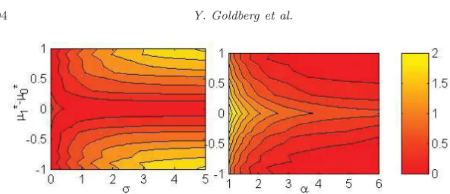
Fig 2. Left: Bias for soft-thresholding. Right: Bias for SoftMax. In both panels the bias is measured in units of 1/√nfor n = 10, as a function of effect size and of the tuning parameters,σ andα, for the soft-thresholding and SoftMax, respectively.

Let Y|A ∼ N(µa,1), a = 0,1, and assume that the treatment assignment is perfectly balanced. We use 1000 Monte Carlo replicates to estimate the bias for each parameter setting. Figure2 below shows the bias as a function of the treatment effectµ∗

1−µ∗0and with tuning parametersσ∈[0,5] andα∈[1,6] for

the soft-thresholding and SoftMax, respectively. It appears that the SoftMax does not suffer from large bias on points away from µ∗

1 −µ∗0 = 0. Also, as

expected from Theorem1, the bias decreases asαincreases.

3. Penalized and adaptive Q-learning

In Penalized Q-learning (Song et al.,2011) and adaptive Q-learning (Goldberg et al.,2013), penalties were imposed on the term H′

2,1β2,1 for each individual.

This use of penalized estimation allows us to simultaneously estimate the second stage parameters and select individuals whose value functions are not affected by treatments, i.e., those individuals whose true values of H′

2,1β2∗,1 are zero.

4. Truncated value function

The non-regularity issue arises primarily in settings where there are some sub-jects who do not respond to treatments at the second stage and where inference focuses on effect size. In the context of public health policy, we think that (i) the overall benefit (value) may be of greater interest compared to individual effect sizes and (ii) those subjects who are not sensitive to treatments (approx-imate non-responders) should not have a large impact on the overall decision making process. Thus, we propose an appropriate alternative criterion, namely theǫ-truncated value, for evaluating the optimal policy as follows:

Vǫ(d1, d2) =Ed[(Y1(d1) +Y2(d2))I(δ(X1)> ǫ, δ(X2)> ǫ)],

where δ(X1) and δ(X2) denote the expected treatment effects at the first and

second stages respectively. Here, ǫ is a small constant indicating a clinically meaningful effect size.

Under a SMART trial with randomization probabilities πk at stagek (k= 1,2), this truncated value is equal to

E[(Y1+Y2)I(A1=d1(X1), A2=d2(X2), δ(X1)> ǫ, δ(X2)> ǫ)/(π1π2)].

Compared to the usual value function, we can see that Vǫ(d1, d2) differs by

at most O(ǫ). Using the Q-learning model, the above value function for the estimated rule is

Vǫ( ˆd1,dˆ2) =

Eh(Y1+Y2)I(A1βˆ1X1>0, A2βˆ2X2>0,|βˆ1X1|> ǫ,|βˆ2X2|> ǫ)/(π1π2)

i

.

One advantage of considering this value function is that non-regularity will no longer be an issue since we have excluded the non-responders from the above statistic. One can easily show√n( ˆVǫ( ˆd1,dˆ2)−Vǫ(d1, d2)) converges to the same

normal distribution under local alternatives whetherP(β2X2= 0)>0 or not.

5. Concluding remarks

We again thank the authors for their very interesting work which likely stim-ulate additional future research on this crucial topic. It is clear that there are many fundamental and unresolved computational, methodological and theoret-ical challenges remaining which will benefit from many diverse problem solving approaches. We look forward to seeing this intriguing research area continue to develop.

Appendix: Proofs

Sketch of proof of Theorem 1. Using the same arguments that lead to Eq. 2 in Laber et al., we have

√

n( ˆβ1−β∗1) = ˆΣ−11PnB1

˘

Y −B′

1β1∗

=S_{n+ ˆΣ}−1

whereS_{n is smooth and asymptotically normal and}

U_{n =}√_n

₁

αnlog

n

1 +eαnH2′,1β2ˆ,1

o

−H′

2,1β2∗,1

+

.

Note that

U_n=√_n

1

αn

logn1 +eαnH2′,1β2ˆ,1o −_α1

n

logn1 +eαnH2′,1β∗2,1

o

+√n

1

αn log

n

1 +eαnH2′,1β2∗,1

o

−H′

2,1β2∗,1

+

= e

αnH2′,1β∗2,1H′

2,1

1 +eαnH′2,1β∗2,1 √

nβˆ2,1−β2∗,1

+oP

_√

nβˆ2,1−β∗2,1

+√nf(αn, H2′,1β∗2,1),

where the last equality follows by taking derivatives, and where

f(α, x) = 1

αlog{1 +e

αx_{} −max(x,0). (1)}

For the remainder term, note that Lemma B.6 shows the consistency of ˆβ2,1,

and that the expectation of the Hessian of 1

αnlog{1 +e

αnH′β_{} is bounded by}

Assumption (A1). Hence, by applying Lemma B.5 to the matrix ˆΣ1that appears

in the remainder term, we conclude that √

n( ˆβ1−β1∗) =Sn+Tn+Wn+oP(1), (2) where

T_{n = ˆΣ}−1 1 PnB1

"

eαnH2′,1β2∗,1 1 +eαnH2′,1β2∗,1

H′

2,1

√

nβˆ2,1−β2∗,1

#

,

W_{n = ˆΣ}−₁1√_nP_{nB1f αn, H}′

2,1β2∗,1

.

Recall that by assumption,αn and thus fact that

eαnx

1 +eαnx →

  

1 x >0

1

2 x= 0

0 x <0

,

we obtain that for a givenh2,1,

eαnh′2,1β2∗,1 1 +eαnh′2,1β2∗,1 →

1h′

2,1β∗2,1>0 +

1 21

h′

2,1β2∗,1= 0 .

Define the functionw:Dp1×l∞(F)×Rp21×[0,1]7→Rp1 byw(Σ, µ, ν, a) = Σ−1_{µ(g(ν, B}

1, H2,1, a)), where

g(ν, b1, h2,1, a) =

  

b1

eh′2,1β∗2,1/a

1+eh′2,1β∗2,1/ah

′

2,1ν

, a >0

b1

(1h′

2,1β2∗,1>0 +121

h′

2,1β2∗,1= 0 )h′2,1ν

and where F={g(ν, b1, h2,1, a),kνk ≤K}. Using the same arguments as those

used in Lemma B.11, one can show that w is continuous at (Σ1,∞, P,Rp21,0).

Thus, using the continuous mapping theorem, it can be shown that S_{n +}T_n

weakly converges to

Σ−1 1,∞

h

G ∞

B1(H2′,0β∗2,0+

H′

2,1β2∗,1

+−B

′

1β1∗)

i

+ Σ−1 1,∞

P B1

H′

2,0Z∞,0+H2′,1Z∞,1 1H2′,1β2∗,1>0 +

1 21

H′

2,1β2∗,1= 0

where

Z′

∞,0,Z′∞,1

′

= Σ−1

2,∞G∞[B2(Y −B2′β∗2)].

We now discuss W_{n, the third term in (3). By Lemma 1(i) below, when}

√

n/αn→0,

Σˆ−1

1 Wn

≤√nP_nΣˆ−1 1

kB1kf(αn, H2′,1β2∗,1)≤

√

nlog 2

αn

P_nΣˆ−1 1

kB1k →0,

which proves (i).

For (ii), letδn →0 such thatαnδn→ ∞. Write

ˆ

Σ1Wn =√nPn B1f αn, H2′,1β2∗,1

1_|H′

2,1β2∗,1|> δn +√nP_{n B1f αn, H}′

2,1β∗2,1

1_|H′

2,1β∗2,1| ≤δn =√nP_{n B1f αn, H}′

2,1β2∗,1

1_|H′

2,1β2∗,1|> δn +√nP_{nB1f αn, H}′

2,1β2∗,1

1_|H′

2,1β2∗,1| ≤δn −1|H2′,1β2∗,1|= 0

+√nP_{n B1f αn, H}′

2,1β∗2,1

1_|H′

2,1β∗2,1|= 0

≡An+Bn+Cn.

Note that by Lemma 1(vi),

kAnk ≤PnkB1k

√

n αn

e−αnδn_→P _0.

Let p(δ) = P 1_|h′

2,1β2∗,1| ≤δ −1

|h′

2,1β2∗,1|= 0 , and note that p(0) = 0

and thusp(δ)→0 asδ→0. Hence,

kBnk ≤P_nkB1k

√

n αn

log(2)k 1_|H′

2,1β∗2,1| ≤δn −1

|H′

2,1β2∗,1|= 0 k P

→0.

Summarizing, we obtain that

W_n→P _a∞log(2)Σ−1 1,∞P B11

|H′

2,1β2∗,1|= 0 ,

Sketch of proof of Theorem 2. Using the same arguments that lead to Eq. 2 in Laber et al., we have

√

n( ˆβ1−β1∗,n) = ˆΣ−11PnB1

˘

Y −B′

1β1∗,n

=S_{n+ ˆΣ}−1

1 PnB1Un, whereS_{n is smooth and asymptotically normal, and}

U_n= e

αnH2′,1β∗2,1,n_H′

2,1

1 +eαnH′2,1β∗2,1,n

√

nβˆ2,1−β2∗,1,n

+oP

_√

nβˆ2,1−β∗2,1,n

+√n

₁

αn

logn1 +eαnH2′,1β2∗,1,n

o

−H′

2,1β2∗,1,n

+

.

Similarly to the proof of Theorem1, we have √

n( ˆβ1−β1∗,n) =Sn+Tn+Wn+oP(1), (3) where

T_{n= ˆΣ}−₁1P_nB1

"

eαnH2′,1β2∗,1,n

1 +eαnH2′,1β2∗,1,nH ′

2,1

√

nβˆ2,1−β2∗,1

#

,

W_{n= ˆΣ}−1 1

√

nP_{nB1f αn, H}′

2,1β2∗,1,n

.

We obtain that for a given h2,1, and β2∗,1,n = β2∗,1+√sn +o(1/ √

n), and αn/ √_n

→a−1

∞,

eαnh′2,1β2∗,1,n

1 +eαnh′2,1β2∗,1,n → 1h′

2,1β2∗,1>0 +

a−1

∞h′2,1s

+1

h′

2,1β∗2,1= 0 .

Using the same arguments given in the proof of Theorem 4.1 ofLaber et al. (see also proof of Theorem1 above) it can be shown that

S_n+T_{n Σ}−1 1,∞

n

G_∞B1(H′

2,0β2∗,0+

H′

2,1β2∗,1

+−B

′

1β1∗)

+P B1 H2′,0Z∞,0+H2′,1Z∞,11H2′,1β∗2,1>0

+P B1 a−_∞1H2′,1s

+1

H′

2,1β∗2,1= 0

o

,

where

Z′

∞,0,Z′∞,1

′

= Σ−1

2,∞G∞[B2(Y −B2′β2∗)].

Note that ˆΣ1Wn can be written as √

nP_{n B1f αn, H}′

2,1β2∗,1,n

1_|H′

2,1β2∗,1|> δn,|αn−1H2′,1s|> δn/2 +√nP_{n B1f αn, H}′

2,1β2∗,1,n

1_|H′

2,1β2∗,1|> δn,|αn−1H2′,1s| ≤δn/2 +√nP_{n B1f αn, H}′

2,1β2∗,1,n

1_|H′

+√nP_{n B1f αn, H}′

2,1β∗2,1,n

1_|H′

2,1β∗2,1|= 0

≡An+Bn+Cn+Dn.

The first three terms can be bounded as follows:

kAn+Bn+Cnk

≤P_nkBk

√

n αn

log(2)k1_|H′

2,1s|> αnδn/2 k+PnkBk √

n αn

e−αnδn/2

+P_nkBk

√_n

αn log(2)

1_|H′

2,1β2∗,1| ≤δn −1|H2′,1β2∗,1|= 0 P

→0.

Thus the limiting distribution of W_{n depends on that ofDn. We have thatDn}

equals

P_nB1

√

n αn

logn1 +e√αn_nH′2,1s+o(1/ √

n)o

−H′

2,1s+o(1)

+

1_|H′

2,1β2∗,1|= 0 P

→P B1

a∞log

n

1 +ea−∞1H2′,1s

o

−H′

2,1s

+

1_|H′

2,1β∗2,1|= 0 ,

which concludes the proof.

Proof of Corollary 1. We prove only the second assertion, the first can be proved similarly. Noting that both S

∞ andT∞have mean zero, it is enough to bound

the bias of

Σ−1

1,∞P(W∞)

= Σ−1 1,∞P B1

a∞log

n

1 +ea−∞1H ′

2,1s

o

−H′

2,1s

+

1_|H′

2,1β∗2,1|= 0 .

Using Lemma 1(i) with α = a−1

∞ and x = H2′,1s, we obtain that the bias is

bounded by

a∞log(2)kΣ−1,1∞kPkBk1

|H′

2,1β2∗,1|= 0 .

The following lemma is needed for the proofs of Theorems1–2:

Lemma 1. Let f(α, x) = _α1log{1 +eαx_{} −max(x,0). Then} (i) 0< f(α, x)≤log(2)/α.

(ii) argmaxxf(α, x) = 0andf(α,0) = log(2)/α. (iii) f(α, x)→0 asα→ ∞.

(iv) Fixδ >0. Then maxx_∈(−∞,−δ]∪[δ,∞)f(α, x) =e

−αδ

α . The proof is technical and therefore omitted.

References

Laber, E. B., Lizotte, D. J., Qian, M., Pelham, W. E., andMurphy, S. A.(2014), Dynamic treatment regimes: Technical challenges and applications. Electron. J. Statist.8 1225–1272.

Moodie, E. E. M. and Richardson, T. S.(2010), Estimating optimal dy-namic regimes: Correcting bias under the null,Scandinavian Journal of Statis-tics, 37, 126–146.MR2675943

Song, R., Wang, W., Zeng, D., and Kosorok, M. R. (2011), Penalized

Q-learning for dynamic treatment regimes,To appear in Statistical Sinica.