Study of Normalization and Aggregation Approaches
for Consensus Network Estimation
Pau Bellot
⇤†, Philippe Salembier
†, Albert Oliveras-Verg´es
†and Patrick E Meyer
‡⇤Email: [email protected]
†Universitat Politecnica de Catalunya BarcelonaTECH, Department of Signal Theory and Communications, Barcelona, Spain ‡Bioinformatics and Systems Biology (BioSys), Universit´e de Li`ege (ULg),
4000, Li`ege, Belgium
Abstract—Inferring gene regulatory networks from expression data is a very difficult problem that has raised the interest of the scientific community. Different algorithms have been proposed to try to solve this issue, but it has been shown that the different methods have some particular biases and strengths, and none of them is the best across all types of data and datasets. As a result, the idea of aggregating various network inferences through a consensus mechanism naturally arises. In this paper, a common framework to standardize already proposed consensus methods is presented, and based on this framework different proposals are introduced and analyzed in two different scenarios: Homogeneous and Heterogeneous. The first scenario reflects situations where the networks to be aggregated are rather similar because the are obtained with inference algorithms working on the same data, whereas the second scenario deals with very diverse networks because various sources of data are used to generate the individual networks. A procedure for combining multiple network inference algorithms is analyzed in a systematic way. The results show that there is a very significant difference between these two scenarios, and that the best way to combine networks in theHeterogeneousscenario is not the most commonly used. We show in particular that aggregation in theHeterogeneous scenario can be very beneficial if the individual networks are combined with our new proposed method ScaleLSum.
I. INTRODUCTION
Inferring gene regulatory networks from expression data is a very difficult problem that has seen a continuously rising interest in the last years and presumably in the years to come due to its applications in biomedical and biotechnological research.
Several studies have compared performances of network-inference algorithms [1], [2], [3], [4], [5], [6], [7], [8], reaching the conclusion that none of the methods is the best across all types of data and datasets. Furthermore, the different algo-rithms have specific biases towards the recovery of different regulation patterns, i.e., Mutual Information (MI) and corre-lation based algorithms can recover feed-forward loops most reliably, while regression and Bayesian Networks can more accurately recover linear cascades than MI and correlation based algorithms [6], [9].
These observations suggest that different network-inference algorithms have different strengths and weaknesses [10]. Therefore, combining multiple network inference algorithms emerges as a natural idea to infer a more accurate gene
regulatory network (GRN), leading to a consensus among Homogeneous networks. We use the term homogeneous here to refer to networks obtained from the same experimental data through the use of different algorithms. But there are other situations where different networks describing the same cells are derived from different original data sets coming from very different technologies such as chip data, microarray, rnaseq and so on. We will refer to this situation as theHeterogeneous scenario.
Behind all state of the art consensus network algorithms one can identify a normalization step followed by an aggre-gation step. The main contributions of this paper are 1) to systematically analyze the combination of normalization and aggregations strategies, creating in some cases new consensus network algorithms and 2) to evaluate the performances of the algorithms in both the Homogeneous and the Heterogeneous scenarios. As will be seen, the conclusions highlight a clear difference in terms of expected performances and algorithm selection in both cases. In order to precisely measure the algorithms performances and to control the degree of homo-geneity without depending on any specific network inference algorithm, we rely on a synthetic network generation method presented in this paper. With this approach we can have a full control on the homogeneity and the characteristics of the individual networks.
II. METHODS
A. State-of-the-art
In order to create a consensus network from initial indi-vidual network inference algorithms, several strategies have been used. Assuming that each algorithm provides a score for each edge of the network, the simplest strategy consists of computing the average of the scores across the N individual networks [11].
Other strategies do not rely on the actual edge scores but on their rank defined in an ordered list. The method proposed in [6] is based on rank averaging: If eij denotes an edge connecting genes i and j and rn(eij) the rank of the edge for network n, the final rank is computed with:
r(eij) = X
1nN
rn(eij) (1)
The consensus network is obtained from the list composed of the sorted values of summed ranksr(eij). This method called
RankSum is also known as Bordacount.
TopkNet [9] is based on the observations made in [6], which showed that integration of algorithms with high-diversity outperform the integration of algorithms with low-diversity [6]. First, for each individual network the predictions are ranked, and then the final rank for each edge is the result of applying a rank filter of orderk, which returns thekth-greatest value (RankOrderFilterk) over all theN values:
r(eij) =RankOrderFilterk{r1(eij), . . . , rN(eij)} (2)
The computation of a rank value in the RankSum and the TopkNet algorithm can be viewed as a normalization of the score values before their aggregation with the sum or the rank order filter. Based on this observation, we present an analysis of potential normalization and aggregation strategies in the following section.
B. Systematic consensus analysis
As previously mentioned, the consensus network estima-tion can be seen as involving two distinct steps. The first one transforms the different network scores, sn(eij), in order to have a common scale or distribution. This process will be referred to as “Normalization”. For example, [6], [9] useRank, whereas [11] does not perform any normalization which can be seen as the Identitynormalization.
Then, the second step is the “Aggregation” of the N different edge scores into one consensus score for every edge. In [6] and [11] this process is done through the Sumprocess, while [9] uses the rank order filter.
We now extend this idea to propose new algorithms. First, different Normalization options are presented, and then the distinct Aggregation proposals are discussed. Finally, their combination will lead to different consensus network algorithm proposals.
1) Normalization:
Five different normalization techniques will be analyzed. Let us call tn(eij)the normalized value assigned to edge eij for the network n.
a) Identity:
The Identitydoes not apply any transformation to the original scores of the inferred network:
tn(eij) =sn(eij) (3)
b) Rank:
The Rank replaces the numerical score sn(eij) by their rank rn(eij)such as the most confident edge receives the highest score. The Rank method preserves the ordering of the scores of inferred links but the differences between them are lost:
tn(eij) =rn(eij) (4)
c) Scale:
A classical normalization of a random variable involves a transformation to remove the effect of the mean value and to scale it accordingly to its standard deviation. The differences between scores are preserved:
tn(eij) =
sn(eij) µn
n
(5)
where µn and n are respectively the mean and standard deviation of the empirical distribution of the inferred scores sn(eij) for network n. This normalization does not assure a limited range of values.
d) RankL:
The previous proposals normalize the whole network only taking into consideration their score values. Extensions of the last two normalizing methods are proposed now. The methods take into consideration the local context of the scores of gene i and j for computing the normalized score of interaction tn(eij). In the RankLmethod (L stands forLocal), two local ranks are initially computed:rn,i(eij)computes the rank of the scoresn(eij)among the scores of all edges connected to gene i, that is the rank of sn(eij) in the list {sn(eil)}l2{1,...,G},
where G is the number of genes in the network. Similarly, the rank of the score sn(eij) among the scores of all edges connected to gene j is computed and denoted by rn,j(eij). Finally, the final normalization is obtained by averaging the two local ranks:
tn(eij) =rn,i(eij) +rn,j(eij)
2 (6)
This normalization is inspired by [12]. Instead of choosing a threshold to get related genes, the authors of [12] propose to use mutual correlation ranks by taking a geometric average of the the two ranks rn,i(eij) and rn,j(eij). They used a “geometric average” to penalize the difference of ranks with a logarithmic manner, but since we do not use correlation ranks, we decided to use the classic arithmetic average.
e) ScaleL:
Finally, following the same type of reasoning, a local version of the scale normalization, called ScaleL, can be defined as:
tn(eij) =q⇣2
i +⇣j2, with⇣i=
sn(eij) µsi
si
,
and⇣j =
sn(eij) µsj
sj
(7)
whereµsi and si denote the mean and standard deviation of
the empirical distribution of the scores of all edges connected to gene i. They are defined as:
µsi =
1 G
G
X
l=1 sn(eil),
si =
v u u t 1
G 1
G
X
l=1
(sn(eil) µsi)
2 (8)
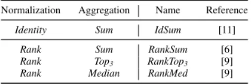
Table I. STATE-OF-THE-ART CONSENSUS NETWORK ALGORITHMS.
Normalization Aggregation Name Reference
Identity Sum IdSum [11]
Rank Sum RankSum [6]
Rank Top3 RankTop3 [9]
Rank Median RankMed [9]
2) Aggregation:
Three different aggregation techniques will be studied. Assume a(eij)denotes the aggregated value of the normalized scores.
a) Sum:
The Sum is a simple summation process that is equivalent to the average of theN values of each link:
a(eij) = N
X
n=1
tn(eij). (9)
b)Top3:
The Top3 is a particularization of the (RankOrderFilterk) with k = 3. We decided to use this particular value based on the observations of [9] which shows that the best integrated networks are obtained with k 2 {5 7} when high number of individual networks are available and there exist several low-performance algorithms. But, when a small number of individual networks are available and none of them has a very small performance compared to the others, then the best integrated networks are obtained with k2{1 3}. Since our synthetic study includes a small number of individual networks and all of them present similar performances (see section III), we are in the second case and therefore, we decided to choose k= 3. The Top3 is the 3rd rank order filter of theN values,
which is defined as taking the 3rd greatest value of the N values of each link:
a(eij) =RankOrderFilter3{t1(eij), . . . , tN(eij)} (10)
c) Median:
Finally, the Median method assigns the median of the N values:
a(eij) = Median{t1(eij), . . . , tN(eij)} (11)
This method could be seen as a particularization of the (RankOrderFilterk) with a fixed value ofk=N/2.
3) Consensus network algorithms:
The combination of 5 possible normalization strategies with 3 possible aggregation rules gives rise to 15 different consensus network algorithms. In terms of nomenclature, the algorithms will be referred to by the two names of the two steps, such that each word or abbreviation of the two steps begins with a capital letter.
Note that some of the combinations give a consensus method that has already been published. These methods are listed in Table I.
III. HOMOGENEOUS VERSUSHETEROGENEOUS NETWORK SCENARIO
TheHomogeneousscenario reflects the case where the in-dividual networks have been inferred with different algorithms but with the same type of data like gene expression as in [6]. In order to get an estimation of the degree of homogeneity that might be expected in this type of scenario, we have downloaded the networks from the supplemental information of [6]. To measure the homogeneity between networks, we have converted them to vectors and computed the correlation between the networks obtaining a mean correlation of 0.6.
On the other hand, the Heterogeneous scenario reflects the case where the individual networks have been inferred from very different kind of data as in [11]. The N individual networks are very different, hardly having any edge in com-mon. To get an estimation of the expected correlation in this scenario, we have downloaded the networks from supplemental material of [11] and converted them to vectors. As before we have computed the correlation between the networks obtaining a mean correlation of 0.06.
A. Synthetic network generation
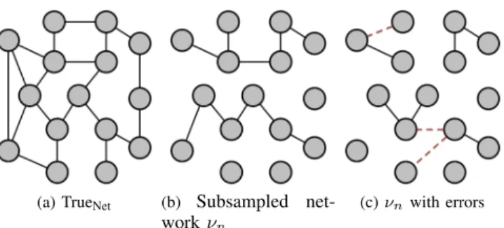
In this scenario, the different consensus methods are meant to be used for the integration networks obtained through the use of real inference algorithms. However, in the present paper we want to precisely and faithfully evaluate the different consensus network alternatives while controlling the degree of homogeneity between networks without depending on any specific network inference algorithm. Therefore, instead of relying on real network inference algorithms, we rely on a subsampling strategy applied on a real network (TrueNet).
1) Homogeneous scenario:
The N individual networks are very similar and have many edges in common. To create the dataset corresponding to this scenario, a unique network is first created by a subsampling of TrueNet. Then, this network is alteredN different times by introducing hard errors (false positives and negatives) and by adding a Gaussian noise to the scores associated to all edges. The alteration parameters are chosen so that the homogeneity of the resulting networks is similar to the one obtained when various inference algorithms are applied on the same data.
2) Heteregeneous scenario:
In this case, the N individual networks are very different and hardly have any edge in common. To reflect this situation, N different networks are generated through various independent subsampling of TrueNet. As previously, these networks are then altered N different times with the introduction of hard errors (false positives and false negatives), and then with soft errors through the addition of Gaussian noise.
3) Subsampling strategy:
(a) TrueNet (b) Subsampled net-work⌫n
(c)⌫nwith errors
Figure 1. Toy example illustration of the first steps of Algorithm 1.
introduced. Following the example and withm= 30, this will introduce 3 false negatives and 3 false positives to obtain ⌘i. The resulting network is presented in Figure 1c, where the dashed lines represent the false positives. The following steps of Algorithm 1 are meant to generate realistic networks, first a Gaussian noise with0mean and standard deviation is added to the network, after this process a constant value is added to shift the scores values in order to ensure non-negative scores in the networks. This step introduces more false positives with a low confidence (if is small) and also introduces variability of the scores in the true “recovered” edges.
Input: TrueNet,Heterogeneous,N
Output:N individual synthetic networks⇣{⌘n}Nn=1
⌘
n 1;
whilen N do
ifHeterogeneous then
⌫n Subsample edges from the TrueNet;
else
ifn==1 then
⌫1 Subsample edges from the TrueNet;
else
⌫n ⌫n;
end end
⌘n Introduce errors in the network⌫n; Add noise to ⌘n;
n n+ 1
end
Algorithm 1:Generate N individual synthetic networks.
IV. EVALUATION PROCESS
A network inference problem can be seen as a binary decision problem. After the thresholding of the network scores, the final decision is a classification: for each possible pair of genes, an edge is defined or not. Therefore, the performance evaluation can be assessed with the usual metrics of machine learning like Receiver Operating Characteristic (ROC) or Pre-cision Recall (PR) curves. In the present paper, we use the Area Under Precision Recall (AUPR) but we do not evaluate the whole network and only take into account the most confident edges, as other papers have already proposed [8], [11], [14]. In order to have statistically significant measures, we choose to evaluate the 20% highest confidence edges as is done in [8], obtaining the AUPR20 measure. We use five different TrueNet networks to evaluate the consensus algorithms, that
Table II. NETWORKS USED IN THIS STUDY AND THEIR CHARACTERISTICS.
Network Name Topology Genes Edges
Rogers1000 R1 Power-law tail topology 1000 1350 SynTReN300 S1 E. coli 300 468 SynTReN1000 S2 E. coli 1000 4695 GNW1565 G1 E. coli 1565 7264
GNW2000 G2 Yeast 2000 10392
Table III. ALGORITHM1PARAMETERS TO GENERATE THE EXPERIMENTAL SETUP.
Parameter Value Number of individual networks (N) 10
Subsampling (t) % 15 Introduced errors (m) % 20 Gaussian standard deviation ( ) 0.3
are generated with three different GRN simulators: GNW simulator [15], SynTReN simulator [16] and Rogers [17]. Four of these networks are real in vivo networks. The main characteristics of these networks are collected in Table II.
V. RESULTS
As mentioned before, the performances of the various algo-rithms are benchmarked with the networks of Table II under the two scenarios described in the previous section:Homogeneous and Heterogeneous network scenarios. In order to generate the individual networks we use the Algorithm 1 with the parameters specified in Table III. Using these values, the mean correlation between the networks in the Homogeneouscase is 0.66 and the mean correlation of the Heterogeneous case is 0.003, which are similar values to the ones obtained in real situations (see section III).
With this experimental setup we generate the individual networks for each one of the networks of Table II, and this procedure is repeated 10 times in order to have different runs of Algorithm 1 and therefore different pools of individual networks.
Since the networks of Table II have different sizes and topological properties, we normalize the AUPR20 of the con-sensus algorithms for each of the 10 runs with the mean AUPR20 of the individual networks (µAUPR20;ind).
AUPR20;norm=
AUPR20 µAUPR20;ind
(12)
With this approach we can compare the different networks. Moreover, it is possible to know if the consensus method is improving on the average network (if AUPR20;normis greater than 1).
Table IV. PERFORMANCES(AUPR20)IN THE HOMOGENEOUS SCENARIO.
R1 S1 S2 G1 G2
µ (⇥103) µ (⇥103) µ (⇥103) µ (⇥103) µ (⇥103)
Individual 0.073 2.919 0.106 4.027 0.192 3.627 0.171 2.096 0.165 2.375 IdSum 0.14 2.74 0.15 6.93 0.274 3.176 0.268 2.198 0.267 3.353 IdTop3 0.128 5.947 0.145 7.397 0.265 5.924 0.257 3.607 0.251 5.446 IdMed 0.135 3.592 0.149 8.423 0.272 3.715 0.262 7.205 0.261 6.036 RankSum 0.118 2.361 0.122 5.72 0.23 3.598 0.226 1.895 0.226 1.925 RankTop3 0.131 3.402 0.148 6.403 0.269 3.762 0.26 2.35 0.258 3.059 RankMed 0.141 3.189 0.151 6.833 0.276 2.871 0.27 2.331 0.268 3.273 ScaleSum 0.14 2.662 0.15 7.097 0.275 3.029 0.269 2.348 0.268 3.213 ScaleTop3 0.131 3.424 0.148 6.307 0.269 3.747 0.26 2.352 0.258 3.057 ScaleMed 0.14 3.226 0.151 6.728 0.276 2.908 0.269 2.333 0.268 3.219 RankLSum 0.12 2.759 0.12 6.077 0.19 5.793 0.171 4.235 0.174 2.44 RankLTop3 0.105 3.556 0.083 8.465 0.104 5.024 0.086 5.45 0.066 1.028 RankLMed 0.138 2.76 0.122 9.425 0.163 4.744 0.14 5.955 0.128 2.06 ScaleLSum 0.142 2.771 0.149 7.045 0.26 3.686 0.25 2.718 0.253 2.823 ScaleLTop3 0.131 3.643 0.143 6.588 0.242 4.09 0.226 2.944 0.229 2.752 ScaleLMed 0.14 3.004 0.147 6.64 0.259 3.701 0.246 2.719 0.249 2.809
Table V. PERFORMANCES(AUPR20)IN THE HETEROGENEOUS SCENARIO.
R1 S1 S2 G1 G2
µ (⇥103) µ (⇥103) µ (⇥103) µ (⇥103) µ (⇥103)
Individual 0.04 1.549 0.062 3.13 0.113 1.611 0.099 1.509 0.094 1.269 IdSum 0.135 6.9 0.203 15.305 0.334 10.795 0.295 8.135 0.282 12.85 IdTop3 0.07 17.018 0.104 16.648 0.185 41.759 0.152 28.039 0.137 35.926 IdMed 0.013 3.6 0.03 7.619 0.047 3.172 0.039 2.38 0.035 9.359 RankSum 0.005 0.811 0.017 3.355 0.021 2.693 0.014 1.328 0.013 1.119 RankTop3 0.131 8.387 0.169 16.796 0.293 6.376 0.27 5.311 0.265 4.463 RankMed 0.01 2.21 0.026 5.883 0.04 3.287 0.033 3.897 0.03 1.619 ScaleSum 0.15 7.287 0.224 15.17 0.362 4.103 0.323 5.796 0.312 5.488 ScaleTop3 0.131 8.389 0.169 16.854 0.293 6.37 0.27 5.319 0.265 4.463 ScaleMed 0.014 2.086 0.031 8.164 0.048 3.855 0.041 4.388 0.038 2.143 RankLSum 0.014 2.741 0.036 5.102 0.12 3.815 0.093 3.851 0.09 3.758 RankLTop3 0.124 6.755 0.156 15.731 0.379 5.437 0.347 5.051 0.368 3.816 RankLMed 0.013 2.558 0.029 5.924 0.128 6.345 0.111 3.82 0.111 3.638 ScaleLSum 0.357 10.392 0.402 17.951 0.641 7.53 0.613 5.855 0.621 4.49 ScaleLTop3 0.124 6.861 0.16 17.092 0.415 4.586 0.391 5.834 0.391 4.31 ScaleLMed 0.019 2.702 0.03 6.62 0.132 5.805 0.119 4.906 0.12 2.971
0.5 1 1.5 2
ScaleLMed ScaleLTop3
ScaleLSumRankLMed RankLTop3
RankLSumScaleMed ScaleTop3
ScaleSum RankMed RankTop3
RankSumIdMed IdTop3
IdSum
Normalized AUPR20
Figure 2. Boxplots Homogeneous scenario.
the results of theHomogeneousscenario while Figure 3 gives the results of theHeterogeneous scenario.
In the homogeneous case, it can be concluded that con-sensus network algorithms allow to improve the inference
0 1 2 3 4 5 6 7 8 9
ScaleLMed ScaleLTop3 ScaleLSumRankLMed RankLTop3 RankLSumScaleMed ScaleTop3 ScaleSum RankMed RankTop3 RankSumIdMed IdTop3 IdSum
Normalized AUPR20
Figure 3. Boxplots Heterogeneous scenario.
making a consensus network. Since, this case almost shows no significant differences between methods, we think that the best option is to use the RankSum [6] or IdSum [11] since they are already part of the state-of-the-art and have a simpler normalization and aggregation methods. However, in the Heterogeneous scenario, we observe large differences between different consensus proposals, where some of them reach worst results compared to the average individual network (Normalized AUPR20 smaller than 1). Observing the figure we can confirm that the IdSum method that was used in [11] in a Heterogeneous scenario is a good choice for this case. But, using the ScaleL as normalization step and Sum as aggregation step provides even better results. It improves the results by6.5(in median) outperforming the improvement of the Homogeneous case, that have a median improvement around of 1.5.
For completeness, the original AUPR20values are shown in table IV and V, presenting the mean and standard deviation for the Homogeneous and Heteregeneous scenarios, respectively. Both tables present the Area Under Precision Recall curve ob-tained in an undirected evaluation on the top 20% (AU P R20%) of the total possible connections for each datasource. The tables also give the mean and variance across the 10 different runs. As can be observed using the parameters of Table III, the individual networks achieve realistic AUPR20 values for these networks [8]. Observing these tables we corroborate the conclusions drawn on Figures 2 and 3.
VI. CONCLUSIONS
In the present paper, we have proposed a framework for combining and integrating different inferred networks. It has been defined as a two step process, consisting in a normaliza-tion strategy followed by an aggreganormaliza-tion technique. We studied two different scenario of practical interest: Homogeneous (sit-uation where various network inference algorithms are used on the same data) andHeterogeneous(situation where various sources of data are used to generate the individual networks), with a controlled synthetic experimental setup. The results show how in a Homogeneous scenario combining individual networks generally outperforms the mean individual network, and that the different analyzed algorithms do not present significant differences. However, in a Heterogeneous scenario the differences are very significant. Many algorithms actually provide results that are worse than individual networks. How-ever, the choice of the proper normalization and aggregation steps allows very large improvements to be obtained. The results show that in this scenario the ScaleLSum is the best option.
ACKNOWLEDGEMENTS
Pau Bellot is supported by the Spanish “Ministerio de Ed-ucaci´on, Cultura y Deporte” FPU Research Fellowship and the Cellex foundation. This work has been done in the framework of the project BIGGRAPH-TEC2013-43935-R, financed by the Spanish Ministerio de Econom´ıa y Competitividad and the European Regional Development Fund (ERDF).
REFERENCES
[1] J. J. Faith, B. Hayete, J. T. Thaden, I. Mogno, J. Wierzbowski, G. Cottarel, S. Kasif, J. J. Collins, and T. S. Gardner, “Large-scale mapping and validation of escherichia coli transcriptional regulation from a compendium of expression profiles,”PLoS Biol, vol. 5, no. 1, p. e8, 2007.
[2] P. E. Meyer, K. Kontos, F. Lafitte, and G. Bontempi, “Information-theoretic inference of large transcriptional regulatory networks,” EURASIP journal on bioinformatics and systems biology, vol. 2007, 2007.
[3] P. E. Meyer, D. Marbach, S. Roy, and M. Kellis, “Information-theoretic inference of gene networks using backward elimination.” inBIOCOMP, 2010, pp. 700–705.
[4] G. Altay and F. Emmert-Streib, “Inferring the conservative causal core of gene regulatory networks,”BMC Systems Biology, vol. 4, no. 1, p. 132, 2010.
[5] ——, “Revealing differences in gene network inference algorithms on the network level by ensemble methods,”Bioinformatics, vol. 26, no. 14, pp. 1738–1744, 2010.
[6] D. Marbach, J. C. Costello, R. K¨uffner, N. M. Vega, R. J. Prill, D. M. Camacho, K. R. Allison, M. Kellis, J. J. Collins, G. Stolovitzky et al., “Wisdom of crowds for robust gene network inference,”Nature methods, vol. 9, no. 8, pp. 796–804, 2012.
[7] S. R. Maetschke, P. B. Madhamshettiwar, M. J. Davis, and M. A. Ragan, “Supervised, semi-supervised and unsupervised inference of gene regulatory networks,”Briefings in bioinformatics, p. bbt034, 2013. [8] P. Bellot, C. Olsen, P. Salembier, A. Oliveras-Verg´es, and P. E. Meyer, “Netbenchmark: a bioconductor package for reproducible benchmarks of gene regulatory network inference,” BMC bioinformatics, vol. 16, no. 1, pp. 1–15, 2015.
[9] T. Hase, S. Ghosh, R. Yamanaka, and H. Kitano, “Harnessing diversity towards the reconstructing of large scale gene regulatory networks,” PLoS Comput Biol, vol. 9, no. 11, p. e1003361, 11 2013.
[10] D. Marbach, R. J. Prill, T. Schaffter, C. Mattiussi, D. Floreano, and G. Stolovitzky, “Revealing strengths and weaknesses of methods for gene network inference,” Proceedings of the National Academy of Sciences, vol. 107, no. 14, pp. 6286–6291, 2010.
[11] D. Marbach, S. Roy, F. Ay, P. E. Meyer, R. Candeias, T. Kahveci, C. A. Bristow, and M. Kellis, “Predictive regulatory models in drosophila melanogaster by integrative inference of transcriptional networks,” Genome research, vol. 22, no. 7, pp. 1334–1349, 2012.
[12] T. Obayashi and K. Kinoshita, “Rank of correlation coefficient as a comparable measure for biological significance of gene coexpression,” DNA research, vol. 16, no. 5, pp. 249–260, 2009.
[13] P. Bellot and P. E. Meyer, “Efficient combination of pairwise feature networks,” inNCW2014 ECML, 2014.
[14] S. Roy, J. Ernst, P. V. Kharchenko, P. Kheradpour, N. Negre, M. L. Eaton, J. M. Landolin, C. A. Bristow, L. Ma, M. F. Linet al., “Iden-tification of functional elements and regulatory circuits by drosophila modencode,”Science, vol. 330, no. 6012, pp. 1787–1797, 2010. [15] T. Schaffter, D. Marbach, and D. Floreano, “Genenetweaver: in silico
benchmark generation and performance profiling of network inference methods,”Bioinformatics, vol. 27, no. 16, pp. 2263–2270, 2011. [16] T. Van den Bulcke, K. Van Leemput, B. Naudts, P. van Remortel, H. Ma,
A. Verschoren, B. De Moor, and K. Marchal, “Syntren: a generator of synthetic gene expression data for design and analysis of structure learning algorithms,”BMC bioinformatics, vol. 7, no. 1, p. 43, 2006. [17] S. Rogers and M. Girolami, “A bayesian regression approach to the
inference of regulatory networks from gene expression data,” Bioinfor-matics, vol. 21, no. 14, pp. 3131–3137, 2005.