Understanding the Cash Demand Puzzle
Janet Hua Jiang
yBank of Canada
Enchuan Shao
zBank of Canada
June 3, 2014
Abstract
We develop a model to explain a puzzling trend in cash demand in recent years: the value of bank notes in circulation as a percentage of GDP has remained stable despite decreasing cash usage at points of sale owing to competition from alternative means of payment such as credit cards. The main feature of the model is that cash circulates between economic activities where the substitutability between cash and other means of payment is uneven. Our model predicts that, once credit expands beyond a certain level, agents adjust their cash management practices in response to further credit expansions, causing the ve-locity of cash to slow down, so that the demand for cash can remain flat despite diminishing cash transactions.
JEL codes: E41, E51
Keywords: Demand for Cash, Credit, Velocity
For their comments and discussions, we would like to thank Jonathan Chiu, Ben Fung, Scott Hendry, Miguel Molico, Hector Perez-Saiz, Lukasz Pomorski, Francisco Rivadeneyra, Gerald Stuber, Liang Wang, Russell Wong, and participants at the Search and Match Workshop in Marrakesh, the Midwest Macro Meetings in Columbia, and the seminars at the Bank of Canada, University of Iowa and University of Hawaii. The views expressed in the paper are those of the authors. No responsibility for them should be attributed to the Bank of Canada.
1
Introduction
The retail payment landscape has undergone significant changes in the past few decades with the emergence of various new payment instruments. In particular, cash has been losing ground to other means of payment at the point of sale. For example, according to Arango et al. (2012), in Canada, cash accounted for nearly 80% of the volume and more than 50% of the value of point-of-sale transactions in the early 1990s; in 2011, these numbers dropped to about 40% and less than 20%, respectively.1 The reduction in cash usage has been picked up by an expanded usage of competing payment methods. For instance, during the same period, the share of credit card payments rose from about 10% to more than 20% in volume, and from less than 40% to 50% in value. Given the diminishing popularity of cash usage at points of sale, one would expect the demand for cash to decrease. However, the total demand for cash, measured as the value of bank notes in circulation as a percentage of GDP, has remained more or less flat at around 3.5% in the past three decades (see Figures 4 and 5 in Fung et al. 2014).
Similar trends are also observed in other countries. For example, Bailey (2009) documents that, in the United Kingdom, the value of bank notes in circulation as a percentage of GDP rose slightly from 2.4% in the mid-1990s to 3.2% in 2009, while cash transactions fell gradually in terms of both volume and value. Recently, Bagnall et al. (2014) have observed the surprising re-silience of cash demand in a group of industrial countries, including Austria, Australia, Canada, Germany and the United States. At the same time, there is evidence that cash transactions have been crowded out by other means of payment. For example, Wang and Wolman (2014) use the scanner data from a large discount chain store in the United States from April 2010 to March 2013, and find that the fraction of cash transactions fell at a rate of between 1.3% and 3.3% per year, depending on the size of transactions. The Reserve Bank of Australia conducted two con-sumer payments use diary studies in 2007 and 2010, respectively. During the period, the share of the number (value) of cash transactions decreased by 6% (5%) (see Bagnall et al. 2011). In addition, the Reserve Bank of Australia Payments System Board Annual Report (2013) shows that from 2004 to 2013, cash usage measured by the value of cash withdrawals grew much more slowly than household consumption.
The main purpose of this paper is to construct a model to reconcile these puzzling
observa-1There are in general three approaches to estimate the value of cash transactions at points of sale: using ATM
tions. The model has two main features. The first is that substitutability between cash and other means of payment is uneven across different economic activities. While alternative means of payment directly compete with cash in many point-of-sale transactions, they are less-ideal sub-stitutes for cash in the underground economy, bars, casinos, or in activities where agents desire anonymity or where unbanked or underbanked agents are involved. We capture this asymmetry by modelling an economy with two sectors: a cash-credit sector, where both cash and credit cards can be used as means of payment, and a cash-only sector, where credit is not accepted.2 The cash-credit sector resembles point-of-sale transactions where cash is subject to intensive competition from other means of payment; the cash-only sector captures cash-intensive activi-ties, where it is hard for other means of payment to compete with cash.
The second main feature of our framework is to emphasize that, during each cycle that cash circulates in the economy, it is likely to be used for a sequence of transactions, where cash and other means of payment may have different extents of substitutability. In particular, in our model, some cash is used first in the cash-credit sector and then again in the cash-only sector. In other words, some agents receive cash revenues in the cash-credit sector to spend in the ensuing cash-only sector: imagine taxi drivers acquiring cash from passengers to dine in cash-only restaurants, bakeries receiving cash from customers to purchase ingredients at local farmers’ markets, farmers selling produce in cash to pay unbanked temporary workers, firms using cash revenues to pay suppliers, etc.3
Our model predicts that, once credit expands beyond a certain level, agents adjust their cash management practices in response to further credit expansions, causing the velocity of cash to slow down, so that the demand for cash can remain flat despite diminishing cash transactions. The intuition is as follows. As credit expands, agents who are buyers in the cash-credit sector hold less cash (to spend in that sector). At the same time, sellers in the cash-credit sector, who rely on cash revenues in that sector to finance their purchases in the cash-only sector, have to acquire more cash in advance to make up for the shortfall of cash receipts in the cash-credit sector. Compared with cash acquired by buyers, which is used in both sectors, cash acquired by sellers has a lower velocity because it is only used in the cash-only sector. Following a credit expansion, cash demand by agents who are sellers in the cash-credit market, which has a lower velocity, constitutes a higher fraction of the total demand for cash. As a result, the overall
2In the real world, many people use credit cards not for the borrowing function but rather for the payment
function. Our model of credit is consistent with this fact since agents do not revolve their debts in the model.
3According to a study by the Canadian Federation of Independent Business (2011), 13% of small and medium
velocity of cash decreases, and the total demand for cash stays constant even if the value of the cash transactions falls.
More generally, our study contributes to the monetary theory literature by showing the im-portance of modelling how cash circulates between economic activities featuring non-uniform substitutability between cash and alternative means of payment. Compared with standard mon-etary models, such as the overlapping-generations model of Samuelson (1958), the cash-in-advance model in Lucas and Stokey (1987), and the monetary search model in Lagos and Wright (2005), our model has very different implications about how credit expansion affects cash velocity, allocation and money demand.
Standard monetary models predict that, in the absence of precautionary demand, the velocity of cash is fixed in each trading cycle, and, therefore, is not affected by credit expansions. In our model, cash functions as a medium of exchange in two subsequent markets. Some part of cash is first used in the cash-credit sector and then reused to finance spending in the cash-only sector; this part of cash has a higher velocity. Our model predicts that credit expansions (beyond a certain level) reduce the amount of cash circulating in both sectors, or the part of cash that involves a higher velocity. Consequently, the overall velocity of cash decreases in response to credit expansions. As for the demand for cash, in a standard model where credit competes with cash in a single market subject to a credit limit (see Gu et al., 2014), credit expansions through relaxed credit limits reduce the demand for cash monotonically, until cash is completely driven out of circulation, a result incompatible with the recent trend in cash demand. In contrast, our model is able to capture the puzzling observation that total cash demand remains flat despite diminishing cash transactions. Regarding allocation, the standard Lagos and Wright (2005) model predicts that, in a monetary economy, the allocation is determined by the inflation rate and is invariant to the credit level. Our model generates a different prediction, suggesting that credit expansions may affect the allocation in a monetary economy by expanding (reducing) trading in the cash-credit (cash-only) sector.
The rest of the paper is organized as follows. Section2describes the environment. Section
3characterizes the equilibrium allocation and examines the effect of credit expansions. Section
2
Economic Environment
Time is discrete and runs from0to1. Each periodt consists of three sequential competitive markets. The first is a settlement market where agents settle debt obligations and adjust money holdings. Following the settlement market, there is a cash-credit market where both cash and credit can be used for transactions. The third market is a cash-only market where only cash is accepted as the means of payment.4 As discussed in the introduction, the structure reflects the
different extent of substitutability between cash and credit across different economic activities. Credit competes directly with cash in the cash-credit market, but not in the cash-only market.
There are three types of infinitely-lived agents, each of measure1. Type A agents are active in all three submarkets. Type B agents participate in the settlement market and the cash-credit market, but do not participate in the cash-only market. Type C agents are active in the settlement market and the cash-only market, but do not participate in the cash-credit market. There is a single perishable good in each market: goodxin the settlement market, goodqin the cash-credit market and goodyin the cash-only market.
In the settlement market, all agents can consume or produce goodx. The utility from con-sumingxunits of the settlement market good isx. Ifx < 0, it means that the agent produces and incurs disutility. In the cash-credit market, type A agents are sellers, who can produce but do not want to consume, and the cost of producingqunits of goods isq. Type A agents are buy-ers, who would like to consume but cannot produce, and their utility from consumingqunits of the good isv(q), withv0 >0, v00 <0andv0(0) =1. The coefficient of relative risk aversion, q = qv00(q)=v0(q), is less than 1everywhere. There exists q such that v0(q ) = 1. In the
cash-only market, type C agents are endowed with a productive technology and can producey
units of good at a cost of y, but do not want to consume. Type A agents cannot produce but would like to consume; their utility from consumption isu(y), withu(0) = 0,u0 >0,u00 <0
andu0(0) = 1. The coefficient of relative risk aversion,
y = yu00(y)=u0(y), is less than1
everywhere. There existsy such thatu0(y ) = 1. Assume thaty < q , or the cash-only
sec-tor is small relative to the cash-credit secsec-tor. The discounting facsec-tor between two consecutive
4The environment differs from the standard Lagos and Wright (2005) or Rocheteau and Wright (2005) model
periods is 2(0;1). To summarize, the lifetime utility of the three types of agents is
Type A : UA= 1 X
t=0 t
[xt qt+u(yt)];
Type B : UB = 1 X
t=0 t[x
t+v(qt)];
Type C : UC = 1 X
t=0 t(x
t yt):
The structure of the economy implies that there are potential gains from trade between type A (as sellers) and type B (as buyers) in the cash-credit market, and type A (as buyers) and type C agents (as sellers) in the cash-only market. There are two payment instruments: money and credit. We assume that type A and B agents can use either cash or credit to trade good
q in the credit market, and that type C agents only accept cash for payment in the cash-only market (from type B agents). The stock of money, Mt, grows at a constant gross rate, Mt+1=Mt. We assume that > . The expansion (contraction) of money supply is
implemented as lump-sum transfers to (taxes on) type B agents in the settlement market in the amount of = ( 1)M. Credit is extended in the cash-credit market, and credit balances are settled in the next period’s settlement market. There is a credit limit such that the debt level in the settlement market cannot exceed` 0. Credit expansion is modelled as an increase in`.5
In each trading cycle, type A agents engage in the following activities. In the settlement market, they choose how much cash to take (to spend in the cash-only market), settle credit balances that they granted in the previous credit-market. In the cash-only market, they use cash to buy goodyfrom type C agents. The activities of Type B agents are as follows. They decide how much cash to take to spend in the cash-credit market, and buy goodqfrom type A agents in the cash-credit market using either cash, credit or both. For type C agents, they sell goody
to type A agents in the cash-only market, and spend money earned in the cash-only market to purchase goodxin the settlement market. The timing of events is summarized in Figure1.
5In the appendix, we discuss the alternative specification that credit expansion manifests as an increase in the
3
Characterization
In this section we characterize the equilibrium allocation and discuss the effect of expanding credit usage. The value functions are denoted as W in the settlement market, V in the cash-credit market andU in the cash-only market. The initial money holding ismin the settlement market,m^ in the cash-credit market and m~ in the cash-only market. To simplify notation, we omit the time subscript. In the case where variables in the current period and the next period are involved, we label variables in the next period with a subscript “+." We first analyze decisions in the settlement market, then the cash-only market and finally the cash-credit market.
3.1
Settlement Market
Normalize the price of the settlement market good, x, to1, and use to denote the value of a dollar measured in units ofx.
3.1.1 Type A Agents
In the settlement market, type A agents settle debt balances incurred in the cash-credit market in the previous period, and adjust cash holdings to carry into the cash-credit market. The value function of a type A agent who enters the settlement market holdingm units of money anda
( 0) units of IOUs is
WA(m; a) = max
x;m^ x+VA( ^m)
s.t. x+ m^ = m+a;
The value function can be rewritten as
WA(m; a) = max
^
m (m m^) +a+VA( ^m): (1)
The first-order condition is
dVA( ^m)
For type I agents, the marginal value of money in the settlement market is
dWA(m; a)
dm = ;
and the marginal value of IOUs is
dWA(m; a) da = 1:
3.1.2 Type B Agents
In the settlement market, type B agents settle debt balances incurred in the cash-credit market in the previous period, and adjust cash holdings to carry into the cash-credit market. The value function of a type B agent who enters the settlement market holdingm units of money anda
( 0) units debt is
WB(m; a) = max
x;m^ x+VB( ^m)
s.t. x+ m^ = (m+ ) a;
where is the lump-sum transfer of money from the government. The value function can be rewritten as
WB(m; a) = max
^
m (m+ m^) a+VB( ^m): (3)
The first-order condition is
dVB( ^m)
dm^ , with equality ifm >^ 0. (4)
For type B agents, the marginal value of money in the settlement market is
dWB(m; a)
dm = ;
and the marginal value of debt is
dWB(m; a)
3.1.3 Type C Agents
The value function for a type C agent in the settlement market is
WC(m) = max
x;m^ x+UC( ^m)
s.t.x = (m m^):
Remember that type C agents do not enter the cash-credit market and go from a settlement market directly to a cash-only market. It can be shown that in the settlement market, type C agents spend all money earned in last period’s only market and take no money to the cash-only market (i.e., m^ = 0) if > , which implies a positive nominal interest rate. Type C agents are sellers in the cash-only market and do not need to use money in that market, so they choose not to take money to that market if the nominal interest rate is positive. Following the above argument, we can write the value function for a type C agent in the settlement market as
WC(m) = m+UC(0); (5)
whereUC is the value for a type C agent in the cash-only market. The marginal value of money
for a type C agent in the settlement market is
dWC(m)
dm = :
Note that owing to linear preferences in the settlement market, all agents of the same type carry the same amount of money at the end of the settlement market, and the marginal value of
mis the same for all three types of agents.
3.2
Cash-Only Market
3.2.1 Type C Agents
In the cash-only market, type C agents sell goodyto type I agents for cash. The value function for type C agents is
UC(0) = max
y;m+
y+ WC(m+)
s.t. y = m+,
whereyis the production of goody, andm+is the money balance that type C agents carry into
the next period’s settlement market. The first-order condition is
= +. (6)
While deciding how much money to earn on the cash-only market, type C agents weigh the marginal benefit and marginal cost of earning one additional unit of cash. The marginal cost to produce one unit of goody entails a cost of1. The marginal benefit is to earn1= units of money and consume += units of good xin the settlement market in the next period, which generates += units of utility. Type C agents will choose (y; m+) by equating the marginal
cost and marginal benefit, which implies equation (6).
3.2.2 Type A Agents
Type A agents decide how much good y to buy and how much money to carry into the next period’s settlement market (credit balances can only be settled in the settlement market). Their value function is
UA( ~m; a+) = max
y;m+
u(y) + WA(m+; a+)
= max
y;m+
u(y) + [ +m++a++WA(0;0)]
s.t.
(
y= ( ~m m+); m+ 0:
If the cash constraint binds, then
If the cash constraint is loose, then
u0(y) = 1ory=y .
The cash constraint binds if and only ifm < y =~ ( +). The value function for type A agents can be rewritten as
UA( ~mj; a+) = 8 < :
u(y ) y + [ +m++a++WA(0;0)]; ifm~ y =( +);
u( +m~) + [a++WA(0;0)]; ifm~j y =( +):
(7)
The marginal value of money is
@UA( ~m; a+)
@m~ = +u
0(y) (
= +, ifm~ y =( +);
> +, ifm < y =~ ( +): (8)
The marginal value of credit extended to others is
@UA( ~m; a+) @a+
= : (9)
3.3
Cash-Credit Market
In the cash-credit market, type A agents (as sellers) and type B agents (as buyers) trade good
q. Let be the value of settlement market goods in the next period,x+, in terms of cash-credit
market goods in the current period,q. Denote! as the value of money in terms ofq. Taking prices as given, type A agents decide how much goodq to produce, and type B agents decide how much to consume.
3.3.1 Type A Agents
Type A agents sell goodqin the cash-credit market to receive money or/and credit as payment. Type A’s value function is
VA( ^m) = max
q;d;a+
q+UA( ^m+d; a+) (10)
wheredis the amount of cash that type A agents receive, anda+is the amount of credit extended
to others that will be repaid in the next period’s settlement market. Letm~ = ^m+dbe the amount of money carried to the cash-only market. The first-order conditions satisfy
d : != @UA( ~m; a+)
@m~ = +u
0(y); (12)
a+ : =
@UA( ~m; a+) @a+
= ; (13)
where the second equalities in equations (12) and (13) use equations (8) and (9), respectively. The value functionVA( ^m)has the following envelope result:
dVA( ^m)
dm^ =! =
@UA( ~m; a+)
@m~ = +u
0(y): (14)
3.3.2 Type B Agents
Letddenote the amount of cash that type B agents spend in the cash-credit market,m~ = ^m d
the remaining cash that type B agents carry to the following settlement market, and a+ the
amount of debt incurred by type B agents to be paid back in the following settlement market. We can express type B agents’ value function in the cash-credit market as
VB( ^m) = max
q;d;a+
v(q) + WB( ^m d; a+) (15)
s.t.
8 > < > :
q =!d+ a+;
0 d m;^
a+ `;
(16)
where the three constraints are the budget constraint, the cash constraint and the credit con-straint, respectively.
If > , then type B agents prefer to use credit whenever possible. If ` q = , then type B agents choose to carry no cash to the cash-credit market, and use only credit to buyq
units of goodq. If` < q = , then type B agents carry positive cash balances to the cash-credit market and spend all of it: with > which implies a positive nominal interest rate, agents will not hold idle cash balances across periods. The value function for the buyer,VB( ^m), has
the following envelope result:
dVB( ^m) dm^ =v
3.4
Equilibrium
We focus on the steady-state equilibrium where real variables are constant over time. The equilibrium gross inflation rate is equal to the money supply growth rate, . The nominal interest rate is = 1 >0under the assumption > . We measure the demand for cash as the real cash balances in terms of the settlement market goodxthat type A and B agents acquire at the end of the settlement market (note that type C agents are sellers in the cash-only market and choose not to carry cash at the end of the settlement market if the nominal interest rate is positive). UsezA = m^AandzB = m^B to denote the cash demand by type A and B agents,
respectively. The total money demand is calculated as z = zA+zB. The total value of cash
transactions (in both the cash-credit market and the cash-only market) is
zT =zB+ y
=zB+ y:
We define the velocity of cash, , as the ratio of the total value of cash transactions,zT, over the
total demand for cash (all measured in terms ofx), i.e.,
= zT
z =
zB+ y
z =
zB+ y
z ; (18)
where the second equality uses (6). The value of GDP (measured in units ofx) is
Y = q
! + y
:
We define the ratio of the value of notes in circulation over GDP as
= z
q
! +
y :
The demand for cash at the end of the settlement market is characterized by
Type A: !, with equality if and only ifzA>0; (19)
Type B : !v0(q), with equality if and only ifzB>0; (20)
(utility) cost of ! (remember that is the value of money in terms of the settlement market goodx, and that! is the value of money in terms of the cash-credit market good q). Type A agents’ demand for cash is positive only if = !. In the settlement market, type B agents acquire cash to spend in the cash-credit market; their demand for cash is positive as long as the credit constraint binds in the cash-credit market, or` < q = . IfzB >0, type B agents equate
the marginal cost of acquiring cash, , to the marginal benefit, which allows them to buy!units of goodqin the cash-credit market, or enjoy!v0(q)units of utility.
Type A agents’ decision to carry money from the cash-credit market to the cash-only market can be derived from (8) and the Euler equations (12):
Type A:!= +u0(y): (21) Under the assumption thatu0(0) = 1, type A agents choose to enter the cash-only market with
positive money balances. In the cash-only market, depending on the amount of cash receipts in the credit market, type A agents may or may not spend all their cash receipts in the cash-only market: their cash constraints may be loose in the cash-cash-only market if they receive large amounts of cash in the cash-credit market, in which case,y=y . In the cash-credit market, type B agents always choose to spend all their money: if > , which implies a positive nominal interest rate, agents will never hold idle cash balances across two settlement markets.
In general, the economy goes through four regimes as`increases and drives out cash trans-actions in the cash-credit market. When the credit limit is small, type B agents choose a large money balance in the settlement market to prepare for trading in the cash-credit market. Given the positive nominal interest rate, the trading in the cash-credit market and the cash-only market lies below the efficient level, i.e.,q < q . For type A agents,q < q implies that > !, or that it is cheaper to acquire cash in the cash-credit market than in the settlement market. As a result, type A agents choose not to hold cash while entering the cash-only market and rely solely on cash receipts in the cash-credit market to finance purchases ofyin the cash-only market. When the credit limit is small, a large amount of trading is carried out in cash in the cash-credit market, which means that type A agents may receive more than enough cash revenue in the cash-credit market to have a loose cash constraint in the cash only market, ory=y . We call this situation I.
market, causing type A agents’ cash revenue to decrease. At some point, type A agents have a binding cash constraint in the cash-only market, andy < y . When this happens, the economy transitions into situation II.
If the credit limit continues to rise, then it is possible that type B agents are able to purchase
q in the cash-credit market (but still pays part of the consumption ofqin cash). Onceq =q , the economy enters into situation III. In this situation, =!, and type A agents take a positive amount of cash from the settlement market to the cash-credit market to compensate for the lower cash revenue in the cash-credit market.
Finally, the credit limit may be so high that the credit constraint becomes loose in the cash-credit market. In this situation (situation IV), transactions in the cash-cash-credit market are entirely conducted in credit (and the amount of trading is at the efficient level q ). Type B agents’ demand for cash becomes zero, and type A agents acquire cash in the settlement market to spend in the cash-only market.
To summarize, as`gradually increases, the economy goes through four situations depending on whether y is equal to or less than y , whether q is equal to or less than q , and whether the credit constraint binds in the cash-credit market (see Table ??). Next, we characterize the equilibrium allocation and discuss the effect of credit expansions in each of the four situations.
Situation y q =! zA Credit constraint zB
I y < q >1 0 bind >0
II < y < q >1 0 bind >0
III < y q 1 >0 bind >0
IV < y q n/a >0 loose 0
3.4.1 Situation I: Low Credit Regime
In the first situation, type A agents receive enough cash in the cash-credit market such that their cash constraint is loose in the cash-only market; as a result, they purchase
y =y (22)
and the marginal benefit of acquiring one additional unit of cash, which implies the relationship
! = +:
We can then determine the output in the cash-credit market by combining type B agents’ deci-sion with type A agents’ decideci-sion. is determined by
=!v0(q) = +v0(q);
or
q=q ; (23)
withq solving
v0(q ) = : (24)
With > , type B agents consume less thanq in the cash-credit market, which implies that type B agents’ valuation of goodqis higher than that of goodx. Consequently, they are willing to pay a higher price for goodqthan for goodx. For type A agents, given that the marginal cost of producing goodq and xis the same, it is cheaper to acquire cash in the cash-credit market than in the settlement market. Type A agents, therefore, choose to acquire zero money balances in the settlement stage (zA= 0), and finances spending on the cash-only market solely by cash
receipts in the cash-credit market. With a very low credit limit, type A agents receive enough cash revenue in the cash-credit market to supporty in the cash-only market.
In situation I, money demand is described by
zB =
q `
! =
q `
+
= (q `); (25)
zA = 0;
z = zB:
The total value of cash transactions is
zT =zB+ y
The velocity of cash is given by
= zT
z = 1 +
y
q `:
The amount of cash with a higher velocity (of two) is( = )y . GDP (measured in units ofx) is
Y = q
! + y
= (q +y ):
The value of notes in circulation over GDP is
= z
Y =
q `
q +y :
In the cash-credit market, type B agents purchaseq units of good, `of which is paid in credit, and the remaining amount,q `, is paid in cash. The value of cash transactions in the cash-credit market, measured in units of good x, is therefore (q `)=!. Using ! = +, we can derive equation (25). Type A agents do not take money to the cash-credit market. The total demand for cash is determined by the cash demand by type B agents.
Proposition 1 Effect of` in situation I:dq=d` =dy=d` = dzA=d` = 0,dzB=d` = dzT=d` = dz=d`= <0,d =d` >0, andd =d` <0:
In situation I, type A agents do not take cash into the cash-credit market, but they receive enough cash revenue in the cash-credit market to have a loose cash constraint in the cash-only market. As a result, they purchase y units of good y in the cash-only market and take the remaining cash into the next period’s settlement market. When type A agents’ cash constraint is loose in the cash-only market, the marginal benefit of earning extra money in the cash-credit market is determined by the inflation rate, which implies that the amount of trading in the cash-credit market,q, depends solely on the inflation rate.
y = = ( = )y and accounts for an increasing fraction of the total money demand, which decreases in response to credit expansions. As a result, the value of notes in circulation over GDP decreases.
3.4.2 Situation II: Intermediate Credit Regime
In situation II, type B agents consume less thanq in the cash-credit market, which implies that it is still cheaper for type A agents to acquire cash in the cash-credit market than in the settlement market. Type A agents, therefore, choose to hold zero money balances while entering the cash-credit market (i.e.,zA = 0), and finances spending on the cash-only market by cash receipts in
the cash-credit market. This is the same as in situation I. However, in situation II, type A agents do not receive enough cash revenue in the cash-credit market to purchase y units of good in the cash-only market. In this situation, type A agents’ cash constraint in the cash-only market binds, and they spend the entire cash revenue earned in the cash-credit market on goody. Using (21) and (6), we can derive the price ofyin terms of goodqas
!
= +u
0(y) +
=u0(y):
The equilibrium allocation (q; y) is given by
y = q `
! =
q `
u0(y) ; (26)
v0(q)u0(y) = : (27)
Equation (26) says that type A agents exhaust cash revenues earned in the cash-credit market to purchase goodyon the cash-only market. They sellq `units of good in cash, which enables them to buyy = (q `=[u0(y)]in the cash-only market. Equation (27) is derived from (20) and (21).
The money demand is described by
zB =
q `
! =
y
= y
+
= y; (28)
zA = 0;
In situation II, becauseq < q and > !, type A agents do not acquire cash on the settlement market, and the total demand for cash is the same as type B agents’ demand for cash. Note that the value of cash transactions the cash-credit market is equal to that in the cash-only market (equation (28)): type B agents’ spending on the cash-credit market becomes type A agents’ cash revenue, all of which is then spent by type A agents to purchase goodyin the cash-only market. As a result, the total value of cash transactions is
zT = 2zB = 2 y;
and the velocity of cash is constant at
= 2:
The value of GDP measured in units ofxis
Y = q
! + y
= q
u0(y)+y :
The value of notes in circulation over GDP is
= z
Y = y q u0(ys) +y
= 1
1 + u0(qy)y:
When type A agents rely on cash revenue in the cash-credit sector to purchase good y in the cash-only sector and have a binding cash constraint in the cash-only sector, the value of notes in circulation is equal to the value of output in the cash-only sector. The same amount of cash is used to support trading in the cash-credit sector (together with credit transactions). The value of notes in circulation over GDP depends on the output ratio in the two sectors, captured by the termq=[u0(y)y].
The effect of credit expansions is stated in Proposition 2.
Proposition 2 Effect of ` in situation II: dq=d` > 0, dy=d` < 0, dzB=d` = dz=d` < 0, dzT=d` <0,d =d`= 0, andd =d` <0:
Proof. First,d =d`= 0is obvious. Equation (27) implies that
v00(q)dq
dyu
or
dq dy =
v0(q)u00(y) v00(q)u0(y) <0:
Equation (26) implies that
`= [q yu0(y)]= ;
and
d` dq =
1
1 d[yu
0(y)] dy
dy dq :
Following the assumption yu00(y)=u0(y)<1, we have d[yu0(y)]
dy =u
0(y) +yu00(y)>0:
Sinced[yu0(y)]=dy >0anddq=dy <0, we haved`=dq >0;or dq=d` >0:
It then follows that
dy d` =
dy dq
dq d` <0; dzB
d` =
dz d` =
dy d` <0; dzT
d` = 2
dy d` <0:
Finally, becausedq=d` >0,dy=d` <0andd[yu0(y)]=dy >0, we havedh q u0(y)y
i
=d` >0, or
d =d` <0:
An increase in the credit limit relaxes type B agents’ cash constraint in the cash-credit market and allows them to consume more in the cash-credit market (q increases). As type B agents use more credit in the cash-credit market, they acquire less cash in the settlement market (zBdecreases). For type A agents, their cash revenue shrinks, but as long asq < q , it is
in the cash-only market (ydecreases). The total demand for cash also decreases because type B agents carry less cash and type A agents have zero demand for cash. As for the velocity of cash, all of the cash acquired by type B agents are used twice: once in the cash-credit market and once in the cash-only market, so the velocity of cash is fixed at2. A credit expansion increases the value of output in the cash-credit sector relative to the value of output in the cash-only sector (q=[u0(y)y]increases), causing the value of notes in circulation over GDP to decrease.
3.4.3 Situation III: High Credit Regime
As the credit limit continues to rise, type B agents are able to afford more consumption in the cash-credit market. Onceq reachesq , the economy switches to situation III. In situation III, with
q=q ; (29)
and
=!;
type A agents have the same cost of acquiring cash in the settlement market and in the cash-credit market. In this situation, type A agents start to acquire some of their cash in the settlement market. The cash-only market allocation (y) is given by
y=y ; (30)
wherey solves
u0(y ) = : (31)
The demand for money is given by
zA = y
zB = y (q `); (32)
zB =
q `
! =q `; (33)
z = zA+zB = y :
The total value of cash transactions is
The velocity of cash is
= zT
z =
q `+ y
y = 1 +
q `
y :
The value of GDP measured in units ofxis
Y = q
! + y
= q
u0(y )+y :
The value of notes in circulation over GDP is
= z
Y = y q u0(y ) +y
:
The effect of credit expansion in situation III is described in Proposition 3.
Proposition 3 In situation III, dq=d` = dy=d` = dz=d` = 0 = d =d` = 0; dzB=d` = dzT=d`= <0,dzA=d`= >0, andd =d`= 2=( y )<0.
expansions, which is consistent with the recent trend in cash demand that we documented in the introduction.
3.4.4 Situation IV: Non-binding Credit Constraint Regime
If ` ` = q = , then the credit constraint is loose in the cash-credit market. In this situa-tion, all cash-credit market transactions are conducted through credit arrangement, and cash is completely driven out in the cash-credit market. The sole purpose of carrying cash is to finance cash-only market transactions. The allocation (q; y) is fixed and described by
q = q ;
y = y :
The demand for cash is fixed and given by
zA = y ;
zB = 0;
z = zA=zT = y :
The velocity of cash is fixed at
= 1:
The value of GDP measured in units ofxis fixed at
Y = q
! + y
= q
u0(y )+y :
The value of notes in circulation over GDP is fixed at
= z
Y = y q u0(y ) +y
:
Once the credit constraint becomes loose, credit expansions have no further impact on the allo-cation, the demand for cash, the velocity of cash or the value of notes in circulation over GDP (see Proposition 4).
We calculate the cut-off values of`that separate the four situations. The cut-off value of`
that separates situations I and II (denoted by`~)solvesy=y in situation II, orq ` =y , or
~
` = q y :
The cut-off value of` that separates situations II and III (denoted by `^) solves zA = (q
` ) + ( = )y = 0in situation III , i.e.,
^
`= q y = q y u
0(y ) :
Under the assumption that yu00(y)=u0(y) < 1, we have d[yu0(y)]=dy > 0; or y u0(y ) = y > y u0(y ). Together withq < q , we have ` <~ `^. Ifq < y ;i.e., if the inflation rate is high enough, then situation I disappears. Under the assumption thatq > y , we have` >^ 0, so situation II always exists. The cut-off value of`that separates situations III and IV is` =q = .
To summarize, our model predicts that when the credit limit is small, i.e., when ` < `~, credit expansions do not affect the allocation in the economy. The credit expansion beyond
~
`may have real effects on the economy. As described in Proposition 2, when ` 2 [~`;`^], more widespread use of credit expands cash-credit activities (qincreases), shrinks cash-only activities (ydecreases), and crowds out cash transactions in the cash-credit sector and the total demand for cash. However, the trend stops once credit expands beyond`^. Once`exceeds`^, the value of cash transactions in the cash-credit sector continues to decrease owing to credit expansion (until the credit constraint becomes loose, or` ` ), but the real allocation and the total demand for cash become fixed. What happens in our model when` 2 [^`; ` ]is consistent with the recent trend in cash demand that we discussed in the introduction. We depict the effect of credit expansions in Figure2.
3.5
Discussion
about the effect of credit expansions on cash velocity, demand for cash, and allocation. In the following, we sketch the standard Lagos and Wright (2005) model with credit (refer to Gu et al., 2014 for a more detailed analysis) and compare its predictions with those of our model.
In essence, our model reduces to a standard Lagos and Wright (2005) model with credit if we drop the cash-only market and retain only the settlement market and the cash-credit market.6 As a result, the model has only type A and B agents who participate in the settlement market and the cash-credit market, but there are no type C agents. Type A (B) agents are sellers in the cash-credit market, so we call them sellers (buyers). The problems in the settlement market can be formulated in the same way as before (see (1) and (7)). A standard result is that sellers take zero cash balances to the cash-credit market.
Without the cash-only market, agents face different problems in the cash-credit market. The buyer solves the problem
Vb( ^m) = max
q;d;a+
v(qb) + W( ^m d; a+)
s.t.
8 > < > :
q =!d+ a+;
^
m+ d 0; a+ `;
wheredis the amount spending, anda+is the debt incurred to be repaid in the next settlement
market.
If > and`is small (the condition on`will be given later), then both the cash and credit constraints bind, and we have
q = !m^ + `; dVb( ^m)
dm^ = v
0(q)!:
Sellers solve the problem
Vs(0) = max
q;d;a+
q+ W(d; a+)
s.t.q = !d+ a+;
6The cash-credit market and the settlement market in our model correspond to the decentralized market and
wheredis cash revenue, anda+is credit extended to buyers. The first-order conditions are
! = +;
= :
Combining the analysis of decisions on the settlement market and cash-credit market, we can characterize the buyer’s money demand in the settlement market by
= dVb( ^m)
dm^ =v
0(q)!=v0(q) +:
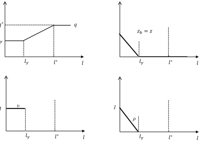
In a stationary equilibrium, the amount of goods being traded in the cash-credit market is given byq =q :The demand for cash is
z = zb =
q `
! = (q `); zs = 0:
The velocity of cash is fixed at = 1:The value of GDP measured in units ofxis
Y = q
! = q:
The value of notes in circulation over GDP is
= z
Y =
(q `)
q = 1
` q :
As` increases, the economy experiences three regimes marked by two cut-off values of`:
` = q = and` = q = . If` ` (regime A), buyers hold positive amounts of money and use both money and credit to purchaseq. Credit expansions do not affect the allocation in this regime: q is fixed at q . Credit crowds out cash usage and cash demand at a constant rate until it becomes zero when` = ` . Once` exceeds ` , the economy becomes a pure credit economy and money demand remains at zero. If` ` ` (regime B),q increases with `
model, which we discuss in more detail below.
In terms of money demand and cash velocity, our model predicts that, once credit usage exceeds a threshold (so that the economy enters into situation III), further crowding out of cash transactions by credit usage induces changes in cash management practices, resulting in lower cash velocity, but has no effect on the demand for cash, a phenomenon observed in many industrialized countries. As credit replaces cash in the cash-credit sector, agents who are buyers in that sector cut down on their cash demand (to be spent in that sector). However, agents who are sellers in that sector make up for the shortfall by acquiring more cash in advance (to spend in the cash-only sector). Because the cash acquired by sellers in advance (which is only used in the cash-only sector) has a lower velocity relative to that acquired by buyers (which is spent in both sectors), the redistribution of money demand from buyers to sellers causes the velocity of cash to decrease. In contrast, in a standard Lagos and Wright model with credit, the velocity of cash is fixed (at one if using the definition in equation (18)). With a fixed velocity, the model predicts that money demand shrinks as credit crowds out cash transactions at a constant rate until the economy transforms into a cashless economy. As a result, the model cannot capture the recent trend in cash demand.
Regarding allocation, the Lagos-Wright model with credit predicts that credit has no effect on allocation in a monetary economy: q is constant at q if z > 0 (which occurs in regime A). In contrast, our model predicts that credit may affect allocation in a monetary economy. If ` < ` <~ `^(or when the economy is in situation II), the demand for money is positive, and a credit expansion enlarges cash-credit market output (and reduces output in the cash-only market).7
Before concluding, we make a few additional comments about our model’s predictions. First, although our main focus is to explain the recent trend in cash demand, our model is also consistent with observations in earlier periods. As shown in Figures 4 and 5 in Fung et al. (2014), the total demand for cash measured as the value of notes in circulation as a percentage of GDP had been decreasing before the1980s, which is consistent with our model’s prediction for the situation with low levels of credit usage (` <`^). To a certain extent, the earlier observations
7Credit expansions have a similar effect on allocation in situation I in our model and in regime A in Lagos and
validate our model.
Second, one may think that with cash playing a diminishing role in the cash-credit sector (cash-credit market), in order to sustain the same level of total demand for cash, activities in the cash-only sector (cash-only market) have to expand to offset the reduced role for cash in the cash-credit sector. Suppose we take a standard cash-good-credit-good model by Lucas and Stokey (1987) and impose credit limits in the cash-credit sector. The set-up resembles our model with one critical difference: cash does not circulate sequentially between the cash-only sector and the cash-credit sector, as in our model. As credit expands in the cash-credit sector, the demand for cash in that sector decreases. Unless the cash-only sector expands, the total demand for cash would decrease. Our model proposes a different mechanism, which does not rely on the expansion of the cash-only sector to support a flat total demand for cash when cash plays a diminishing role in the cash-credit sector: the results listed in Proposition 3 are derived with a fixed size of cash-only market (output is fixed at y ). In our model, cash received in the cash-credit sector re-enters and is reused to finance spending in the cash-only sector. As credit expansion crowds out cash usage in the cash-credit economy, agents who receive cash in the cash-credit sector will face a tighter cash constraint in the cash-only sector and respond by increasing their demand for cash (which has a lower velocity). This force counteracts the diminishing demand for cash to be spent in the cash-credit sector, so that the total demand for cash remains fixed. Given the wide difference in the estimate of the size of the cash-only sector and its trend, it is a desirable feature that our model’s prediction does not hinge on the size of the cash-only sector.8
Third, in our model we focus on the competition between cash and credit, but our story has relevance for other electronic payments, such as debit cards, general purpose pre-paid cards, mobile payments, virtual currencies, etc. A common feature of these increasingly popular pay-ment instrupay-ments is that they are more convenient than cash in some transactions, but they are yet to become the perfect substitute for cash in all activities. Our paper captures these features in a simplistic manner: the substitutability is perfect in the cash-credit sector, and there is zero substitutability in the cash-only sector. We expect that the main forces to generate our results
8For example, the estimate of the size of the underground economy, which tends to be cash sensitive, varies
remain relevant in more general settings where the substitutability between cash and other pay-ment instrupay-ments is modelled in a less-extreme manner. As long as the replacepay-ment of cash by these payment schemes varies across sectors in the economy and some agents use cash re-ceipts from less-cash-intensive sectors to finance more-cash-intensive activities, the mechanism described in our paper would hold.
4
Conclusion
This paper builds a model to reconcile a puzzling recent trend in cash demand: the total demand for cash, measured by the value of notes in circulation as a percentage of GDP, remains more or less flat despite diminishing cash usage owing to intensive competition from other means of payment, such as credit cards. Our model emphasizes that the substitutability between cash and other means of payment is uneven across different economic activities, and that it is important to model how cash circulates across these activities. If some agents use cash receipts in less-cash-intensive sectors to finance spending in more-less-cash-intensive sectors, then the total demand for money may not decrease even if cash plays a diminishing role in transactions. Once the expansion of alternative means of payment exceeds a certain level, agents adjust their cash management practices causing the velocity of cash to fall, so that the demand for cash can remain flat despite diminishing cash transactions.
payment choice surveys.9 Useful (albeit imperfect) aggregate time-series data have also been
constructed to monitor consumers’ cash demand. However, studies on merchants’ cash demand are very limited. Rigorous empirical studies in this area would be valuable.
9For example, see Mooslechner et al. (2006) for the Austrian survey, Bagnall et al. (2011) for the Australian
A
Credit Expansion along the Extensive Margin
In this appendix, we discuss the model’s implication if we model credit expansion along the extensive margin, i.e., as a higher fraction of type B agents using credit cards (with no credit limit). At the beginning of the settlement market, type B agents experience a technological shock: fraction of them have access to credit cards, while the rest do not. In the following, we use subscript “c" to refer to type B agents with credit cards, and “m" to refer to type B agents who have no credit cards and use cash only.
The settlement market and cash-only market problems remain the same as in the main text. In the cash-credit market, type A agents’ problem remains the same, but we need to distinguish between type B agents who have credit cards and those who do not. Agents who have credit cards choose to carry zero cash balances into the cash-credit market (zc = 0), and purchase qc = q using credit incurring a credit balance of q = . The value of a type B agent who uses
only money in the cash-credit market is
Vm( ^mm) = max
qm;;d
v(qm) + Wm( ^mm d)
s.t.
(
qm =!d;
^
mm d 0;
where the two constraints are the budget constraint and the cash constraint, respectively. With
> , type B agents who use cash choose to hold just enough money to spend in the cash-credit market, i.e.,d= ^mm. The value functionVm( ^m)has the following envelope result:
dVm( ^mm) dm~m
=v0(qm)!:
Collect the equations that characterize the equilibrium allocations and prices as follows:
settlement market type B agents without credit : =!v0(qm);
settlement market type A agents : !, with equality ifm^A>0;
cash-credit market type B agents with credit : qc =q ;
The equilibrium allocation(qm; qc; qA; y)is given by
v0(qm)u0(y) = ; (34)
qc = q ; (35)
(y y ) y (1 )qm
u0(y) (qm q ) = 0; (36)
qA = q + (1 )qm: (37)
Similar to the model discussed earlier, there are three situations depending on whether type A agents acquire cash in the settlement market or not, and whether they consume y in the cash-only market or not (situation IV corresponds to the case where = 1).
The velocity of cash is
= (1 )zm+
y
z :
The value of GDP measured in units ofxis
Y = (1 )qm+ q
! +
y :
The value of notes in circulation over GDP is
= z
Y :
A.1
Situation I: Low Credit Regime
In situation I, type A agents do not accumulate cash in the settlement market. They receive enough cash revenue in the cash-credit market to purchasey units of consumption in the cash-only market, i.e.,
y=y :
type B agents who have no credit cards purchaseq units of goods in the cash-credit market, or
In situation I, money demand is given by
zc = 0;
zm = qm
! = q ; zA = 0;
z = (1 )zm = (1 )q :
The value of cash transactions is
zT = (1 )
qm ! +
y
= [(1 )q +y ]:
The velocity of cash is
= zT
z = 1 +
y
(1 )q :
The value of GDP measured in units ofxis
Y = (1 )qm+ q
! +
y
= [(1 )q + q +y ]:
The value of notes in circulation over GDP is
= z
Y =
(1 )q
(1 )q + q +y :
Proposition 5 Effect of in situation I:dqm=d =dqc=d =dy=d = 0,dzT=d =dz=d <0, d =d >0, andd =d <0:
Proof.
dzT
d =
dz
d = q < 0: d
d =
y q
1
(1 )2 >0:
Rewrite as
= 1
Then,
d
d /
dh(1q +)yq i d <0:
A.2
Situation II: Intermediate Credit Regime
In situation II, we still haveqm < q (butqm > q ), and type A agents still do not hold cash.
However, unlike in situation I, type A agents do not have enough cash revenue in the cash-credit market to support consumption ofy on the cash-only market. In this case, type A agents spend all the cash receipts from the cash-credit market to purchasey on the cash-only market. As a result,
y= (1 )qm
! =
(1 )qm
u0(y) :
In situation II, money demand is given by
zc = 0;
zm = qm
! =
y
1 ;
zA = 0;
z = (1 )zm = y:
The value of cash transactions is
zT = 2 y:
The velocity of cash is fixed at
= 2:
The value of GDP measured in units ofxis
Y = (1 )qm+ q
! +
y
= 2y+ q
The value of notes in circulation over GDP is
= z
Y = y
2y+u0q(y):
In situation II, the effect of credit expansions is described in the following proposition.
Proposition 6 Effect of in situation II:dqm=d > 0, dy=d < 0, dz=d < 0, dzT=d < 0, d =d = 0, andd =d <0:
Proof. Fromv0(qm)u0(y) = = , we can derive
v00dqm dy =
u00
(u0)2
anddqm=dy <0ordy=dqm <0. Equationy= (1 )qm=u0(y)implies that = 1 yu0(y)=qm
and
d dqm
=
d[yu0(y)]
dy dy
dqmqm yu
0(y)
(qm)2
>0;
or
dqm=d >0:
It then follows that
dy=d = (dy=dqm)(dqm=d )<0:
For the money demand,
dz=d = ( = )dy=d <0:
For the value of cash transactions,
dzT=d = 2( = )dy=d <0:
Rewrite as
= 1 + 1
1 +y =y:
Then,
d
d /
Rewrite as
= 1
2 + u0(qy)y:
Usingd[yu0(y)]=dy >0anddy=d <0, we have
d
d /
dhu0(y)yi d <0:
A.3
Situation III: High Credit Regime
As the fraction of credit card users continues to increase, cash becomes more scarce in the cash-credit market relative to the settlement market. At a certain point, the value of cash in the two markets is equalized with =!. The economy enters into situation III, and type A agents start to accumulate some cash to make up for the decreasing cash revenue in the cash-credit market. In this situation,qm =q andy=y . The money demand is given by
zc = 0;
zm = q
! =q ; zA =
y
zV = y
+
zV = y (1 )q ;
z = (1 )zm+zA = y :
The value of cash transactions is
zT = (1 )q + y :
The velocity of cash is
= zT
z = 1 +
(1 )q
The value of GDP measured in units ofxis
Y = (1 )qm+ q
! +
y
= q + y :
The value of notes in circulation over GDP is
= z
Y = y
q + y :
The effect of credit expansion in this situation is described in the proposition below.
Proposition 7 Effect of in situation III: dqm=d = dqcd = dy=d = dz=d = d =d = d =d = 0,dzT=d = q <0, andd =d <0:
Once the fraction of type B agents with credit cards exceeds the threshold value^, a further credit expansion reduces the weight of cash transactions in the cash-credit market, but the total money demand curve becomes flat. The reduction in type B agents’ money demand is exactly offset by the rise in type A agents’ money demand.
The cut-off value of that separates situations I and II, denoted by~, solvesy = (1 )q ;
or
~ = 1 y
q :
The cut-off value of that separates situations II and III, denoted by ^, solves y = (1 )q =u0(y ), or
^ = 1 y u0(y )
References
[1] Arango, C., K. P. Huynh, B. Fung, and G. Stuber (2012): “The Changing Landscape for Retail Payments in Canada and the Implications for the Demand for Cash," Bank of
Canada Review, (Autumn): 31-40.
[2] Arango, C., and A. Welte (2012): “The Bank of Canada’s 2009 Methods-of-Payment Survey: Methodology and Key Results," Bank of Canada Discussion Paper No. 2012-6.
[3] Bagnall, J., D. Bounie, K. P. Huynh, A. Kosse, T. Schmidt, S. Schuh, and H. Stix (2014): “Consumer Cash Usage: A Cross-Country Comparison with Payment Diary Survey Data," Bank of Canada Working Paper (forthcoming).
[4] Bagnall, J., S. Chong, and K. Smith (2011): “Strategic Review of Innovation in the Payments System: Results of the Reserve Bank of Australia’s 2010 Consumer Pay-ments Use Study," available at http://www.rba.gov.au/publications/consultations/201106-strategic-review-innovation/pdf/201106-strategicreview-innovation-results.pdf.
[5] Bailey, A. (2009): “Banknotes in Circulation – Still Rising. What does this Mean for the Future of Cash?" Keynote address, Banknote 2009 Conference, Washington DC.
[6] Berentsen, A., G. Camera, and C. Waller (2005): “The Distribution of Money Balances and the Non-Neutrality of Money," International Economic Review, 46, 465-487.
[7] Canadian Federation of Independent Business (2011): “Changing the Way We Pay: Get-ting the Transition Right for SMEs."
[8] Deutsche Bundesbank (2013): “Payment Behavior in Germany in 2011," Technical Re-port, Deutsche Bundesbank.
[9] Dunbar, G. R., and C. Fu (2012): “Income Illusion: Tax Evasion Measurement and a Test," Manuscript.
[10] Foster, K., S. Schuh, and H. Zhang (2013): “The 2010 Survey of Consumer Payment Choice," Federal Reserve Bank of Boston Research Data Report No. 13-2.
[12] Gu, C., F. Mattesini, and R. Wright (2014): “Money and Credit Redux," Manuscript.
[13] Jonker, N., A. Kosse, and L. Hernandez (2012): “Cash Usage in the Netherlands: How Much, Where, When, Who and Whenever One Wants?" De Nederlandsche Bank Occa-sional Studies.
[14] Lagos, R., and R. Wright (2005): “A Unified Framework for Monetary Theory and Policy Analysis," Journal of Political Economy, 113(3), 463-484.
[15] Lucas, R. E. Jr., and N. L. Stokey (1987): “Money and Interest in a Cash-in-Advance Economy," Econometrica, 55, 491-513.
[16] Mooslechner, P., H. Stix, and K. Wagner (2006): “How are Payments Made in Austria? Results of a Survey on the Structure of Austrian Households’ Use of Payment Means in the Context of Monetary Policy Analysis," Monetary Policy and the Economy (Q2), 111-134.
[17] Reserve Bank of Australia (2013): “Payments System Board Annual Report."
[18] Rocheteau, G., and R. Wright (2005): “Money in Search Equilibrium, in Competitive Equilibrium, and in Competitive Search Equilibrium," Econometrica, 73, 175–202.
[19] Samuelson, P. A. (1958): “An Exact Consumption-Loan Model of Interest with or without the Social Contrivance of Money," Journal of Political Economy, 66, 467–482.
[20] Schneider, F., and A. Buehn (2012): “Shadow Economies in Highly Developed OECD Countries: What are the Driving Forces?" IZA Discussion Paper No. 6891.
[21] Terefe, B., C. Barber-Dueck, and M.-J. Lamontagne (2011): “Estimating the Underground Economy in Canada, 1992-2008," Technical Report, Statistics Canada.
cash-credit
Type A (buyers): u(y) $ y
Type C (sellers): y
Type A and B adjust $ and settle IOU: x
Type C spend $: x
cash-only
Type A (sellers): -q
q $,IOU Type B (buyers): v(q)
time
settlement settlement
t t+1
t-1
𝑙̂
𝑙̃ 𝑙∗ 𝑙
𝑙̂
𝑙̃ 𝑙∗ 𝑙
𝑧 𝑧𝐵
Figure 2: Effect of credit expansion
𝑙̂
𝑙̃ 𝑙∗ 𝑙
ρ
𝑙̂
𝑙̃ 𝑙∗ 𝑙
υ
1 1
𝑧𝐴
2 𝑧𝑇
𝑙̂
𝑙̃ 𝑙∗ 𝑙
𝑞𝛾
𝑞∗
𝑙̂
𝑙̃ 𝑙∗ 𝑙
𝑦𝛾
𝑦∗
y
𝑙∗ 𝑙
1
𝑙𝛾
𝑙∗ 𝑙
𝑙𝛾 𝑧𝑏 =𝑧
Figure 3: Effect of credit expansion in Lagos-Wright
𝑙∗ 𝑙
𝑞𝛾
𝑞∗
𝑙𝛾
𝑙∗ 𝑙
1
𝑙𝛾 υ
q