Adoption of a New Payment Method:
Theory and Experimental Evidence
Jasmina Arifovic
John Duffy
yJanet Hua Jiang
zMay 31, 2019
Abstract
We model the introduction of a new payment method that competes with an existing payment method. The new payment method involves relatively lower per-transaction costs for both buyers and sellers, but sellers must pay a fixed acceptance fee. Due to network effects, there are two symmetric pure strategy equilibria in which only one of the two payment methods is used. The equilibrium with the new payment method is socially optimal as it minimizes total transaction costs. In an experiment, we find that, depending on the fixed acceptance fee and on the choices made by participants on both sides of the market, either equilibrium can be selected. A lower fixed acceptance fee favors quick adoption of the new payment method, while for a sufficiently high fee, sellers gradually learn to refuse to accept the new payment method. An evolutionary learning model provides a good characterization of our experimental data.
JEL classification numbers: E42, D14, D83, C72, C92.
Keywords: Payment methods, network effects, e-money, experimental economics.
Department of Economics, Simon Fraser University. Email: [email protected].
yCorresponding author. Mailing address: Department of Economics, University of California, Irvine, 3151
Social Science Plaza, Irvine, CA 92697-5100. Email: [email protected]. Tel: 1-949-824-8341.
1
Introduction
The payments industry has undergone significant changes in the past few decades. Var-ious new means of payments that compete with the traditional payment method – cash – have entered into the payment landscape, including debit cards, credit cards, general purpose pre-paid cards such as Visa and MasterCard gift cards, public transportation cards that have expanded into retail transactions such as the Octopus card in Hong Kong, mobile payments such as M-Pesa in Kenya, online money transfer schemes such as Paypal and Venmo, and virtual crypto-currencies such as Bitcoin and Litecoin. The numerous and varied attempts to introduce new payment methods have met with mixed results. The Octopus card in Hong Kong is a notable success. Danmont in Denmark ultimately failed after a few years of limited success. Mondex debuted with much fanfare in several countries but soon failed. Recently, in many countries (including Canada, China, Norway, Sweden, and the United Kingdom), central banks have been debating whether or not to issue their own central bank digital cur-rency (CBDC). Among the many important issues related to CBDC, one relevant question is whether the CBDC, as a new payment instrument, will be adopted by the public if central banks choose to issue it.
In this paper we study the introduction of a new, lower transaction cost payment method, focusing on electronic paid schemes. CBDC will most likely be in the form of such a pre-paid digital fiat money and so our analysis is directly relevant to the introduction of CBDC.1 We seek answers to several questions. Will this new and socially more efficient payment method take off? Can it replace the existing payment method or merely coexist with cash? Will merchants accept the new payment method? How do consumers make portfolio choices between the existing payment method and the new payment method? How do merchants and consumers’ beliefs matter for payment adoption and are there network feedback effects? How does the cost structure associated with the new payment system affect these results?
We first develop a model of the introduction of a new payment instrument, “e-money,” that competes with an existing payment method, “cash.” We model the new payment method as being more efficient for both buyers and sellers in terms of per transaction costs. Such a cost-saving motive lies behind the various attempts to introduce a new payment method: after all, if the new payment method did not offer any such cost savings, there would be no reason to expect it to be adopted (or even introduced). There is also evidence that new developments in electronic payment technology can greatly speed up transactions and save on various handling costs associated with traditional payment methods. According to a study by Polasik et al. (2013), who analyze the speed of various payment methods from video material
recorded in the biggest convenience store chain in Poland, a transaction using contactless cards in offline mode without slips costs on average 25.71 seconds, a significant reduction over a cash transaction, which costs 33.34 seconds. Arango and Taylor (2008) suggest that, after the various cash-handling costs – including deposit reconciliation, deposit preparation, deposit trips to banks, coin ordering, theft and counterfeit risk, etc. – are accounted for, a cash transaction costs merchants $0.25 and a (PIN) debit transaction costs $0.19.2 Modeling a force that works against the adoption of the new e-money payment method, we assume that sellers have to pay a fixed setup fee (to rent or purchase a terminal) to process the new payment method.
Given the cost structure of the two payment methods, buyers and sellers play a two-stage game. In the first stage, both types of agents make simultaneous payment decisions. Buy-ers allocate their budget between the existing and the new payment methods. SellBuy-ers decide whether or not to pay a one-time fixed cost to accept the new payment method. We main-tain throughout that sellers must always accept the existing payment method as a result of custom or due to legal restrictions. The second stage consists of multiple rounds of meet-ings where buyers and sellers trade with each other. In each meeting, the buyer observes whether or not the seller accepts the new payment method, and the trade is successful if the buyer can use a payment method accepted by the seller. Due to network effects, the model admits two symmetric pure strategy Nash equilibria. In one of these equilibria, the new pay-ment method is not adopted and all transactions continue to be carried out using the existing payment method (cash). In the other equilibrium, the new payment method is adopted and completely replaces the existing payment method. The equilibrium involving only the new payment method is socially optimal as it minimizes total transaction costs (the reduction in per transaction cost exceeds the fixed cost paid by sellers).
As our model always admits multiple equilibria, we next turn to a laboratory experiment to assess the conditions under which the new payment method replaces the existing payment method, and also the conditions under which the new payment method fails to be adopted. We find that, depending on the fixed cost for the adoption of the new payment method and on the choices made by participants on both sides of the market, either symmetric equilib-rium can be selected. More precisely, if sellers face a low fixed cost to adopting the new payment method, then the new payment method is quickly adopted by all participants, while for a sufficiently high fixed cost of adoption, sellers gradually learn to refuse to accept the new payment method and transactions are increasingly conducted using the existing payment method.
We view the experimental approach as a useful complement to theoretical and empirical research on the acceptability of payment methods. The theoretical literature emphasizes the importance of network externalities in the adoption of new payment methods (Rochet and Tirole, 2002; Wright, 2003; McAndrews and Wang, 2012; Chiu and Wong, 2014). For the consumer (merchant), the benefit of adopting (accepting) a new payment method increases if more merchants accept (consumers use) that payment method. These network effects lead to multiple equilibria, which pose a problem for making theoretical predictions, and thus our experimental study can shed some light on which equilibrium is more likely to obtain under certain conditions. While the theory often focuses on equilibrium analysis and ignores transition dynamics, our experimental approach also provides some useful insights about the dynamic process by which a new payment method may take off and the speed with which this may occur.
Beyond observing transition behavior, we further model the dynamic adjustment process using an evolutionary learning model. We find that our model provides a very good fit to the experimental data we collected for the original three experimental treatments of our design. Indeed, the impressive fit of this learning model to our experimental data motivated us to use that model to design and predict outcomes for a fourth experimental treatment. We then carried out that additional experimental treatment and again report a very good fit between the evolutionary model and the experimental data. Thus, our dynamic learning model provides a very good characterization of buyers and sellers’ payment choices even out-of-sample.
There is a large empirical literature using survey data to explore individual choices among different means of payments.3 Limited by the survey data available, these studies focus mainly on choices among existing payment methods and the decisions made by just one side of the payment system, either the consumer or the merchant. Consumer and merchant sur-veys are rarely conducted concurrently, and because of high costs, are usually run at a very low frequency (every few years), making it a challenging task to study the feedback effect between the two sides of the payment system as we do in this paper.4 For example, as dis-cussed in Bounie, François and Van Hove (2017), empirical evidence on how consumer card usage drives merchant card acceptance is mostly indirect. To provide more direct evidence on
3See, for example, Arango, Huynh and Sabetti (2016) for an analysis using the Bank of Canada 2009 Method of Payment Survey, Koulayev et al. (2016) using the Federal Reserve Bank of Boston 2008 U.S. Consumer Payment Choice Survey, and von Kalckreuth et al. (2014) using the Deutsche Bundesbank 2008 Payment Habits in Germany Survey. Recently, Bagnall et al. (2016) studied consumers’ use of cash by harmonizing payment diary surveys from seven countries. In addition to studies using survey data, other research – including Klee (2008), Cohen and Rysman (2013), and Wang and Wolman (2016) – uses scanner data to study payment choices at the point of sale. Compared with survey data, scanner data are less prone to errors and misreporting. However, scanner data are less useful for the study of payment adoption.
4Merchant surveys are even more scarce because it is more difficult to recruit merchants to participate in the
that matter, the authors painstakingly combine three surveys conducted in France: a merchant survey in 2008, and two consumer diary surveys in 2005 and 2011. The feedback in the other direction (from merchants to consumers) has been made relatively easier thanks to improve-ments to recent consumer surveys to include questions on payment instruimprove-ments accepted at the point of sale. Nonetheless, as pointed out in Huynh, Schmidt-Dengler and Stix (2014), special care must be taken to handle the endogeneity of card acceptance: consumers’ choice of vendors may depend on the cash they have on hand.
In our model and experiment, we develop an environment suitable for the study of new payment adoption that considers interactions between both sides of the market (buyers and sellers). A novelty of our approach is that we elicit both buyers and sellers’ beliefs about market conditions that are relevant to payment choices. We are thus able to directly inves-tigate the feedback effect by examining how buyers respond to sellers’ acceptance choices in the past and to buyers’ beliefs about sellers’ decisions in the coming trading cycle (or “market”). Similarly, we can study how sellers’ acceptance decisions depend on their trading experiences with buyers in the past and sellers’ beliefs about buyers’ payment choices in the coming trading cycle. Further, we can examine how the decisions on the two sides co-evolve over time (which is difficult to do with field data because of the low frequency of payment surveys).5
The closest paper to this one is by Camera, Casari and Bortolotti (2016, hereafter CCB), who also develop a model of payment choice between cash and e-money/cards and also con-duct an experimental study. While we take inspiration from CCB’s paper, our project differs from theirs along several dimensions, including the theoretical model, experimental design, research questions and experimental results. CCB study how the presence of proportional seller fees and buyer rewards affects the adoption of “card” payments, which are assumed to be more “reliable” than cash.6 They report that sellers readily adopt card payments,
regard-5Generally speaking, laboratory studies have two additional advantages over studies based on survey data.
First, survey data are subject to errors due to insufficient incentives for truthful or careful reporting, or misun-derstandings about the survey questions posed; these problems are alleviated to some extent in an incentivized experimental study where subjects are quizzed on their understanding of the rules prior to play and paid based on their performance in accordance with the model’s payoff structure. Second, since many factors are at play in the field, isolating the effect of a particular factor can be more challenging. In the laboratory, we can exert better control over the environment, thereby isolating the factors that play a role in whether or not a new payment method is adopted.
less of the fee and reward structure, while buyers are more sensitive to these incentives. More precisely, the buyers’ adoption rate is high in the absence of fees or rewards. Imposing seller fees alone reduces card adoption, but adding buyer rewards neutralizes the effect of seller fees and restores card adoption to high levels. CCB also find that there is little feedback effect between the two sides of the market so that network externalities do not matter for payment adoption. However CCB do not elicit beliefs by market participants about the likely behavior of participants on the other side of the market. Our research question is how the adoption of a new and more socially efficient payment method is affected by the fixed cost borne by sellers relative to the potential saving on per transaction costs as well as by beliefs, which we do elicit. We find that choices by both buyers and sellers depend critically on the magnitude of the seller’s fixed cost of adoption as well as on beliefs about what the other side of the market will do. In contrast to CCB, we find a strong feedback effect between the two sides. Finally, as noted earlier, we also demonstrate that an evolutionary learning model explains our experimental data well and is useful for out–of–sample prediction purposes.
The rest of the paper is organized as follows. Section 2 develops the theoretical model. Section 3 describes our experimental design. The aggregate experimental results are pre-sented in section 4. Individual buyer and seller behavior is examined in section 5. In section 6 we present an evolutionary learning model that can closely track our experimental findings and we use this model to design and predict behavior in a further experimental treatment. Finally, section 7 concludes with a summary and some directions for future research.
2
The Model
In this section, we develop a simple model of the adoption of a new payment method, "e-money," that competes with an existing payment method, "cash." Each market (or trading cycle) consists of two stages. In the first stage, buyers make a portfolio decision, splitting their budget between e-money and cash. Simultaneously, sellers decide whether or not to accept e-money transactions; cash payments must always be accepted. In the second stage, buyers meet pairwise with sellers and engage in transactions using one payment form or the other. For simplicity (and later experimental implementation) we assume homogeneous buyers and sellers, an exogenously given spending budget for the buyer and fixed terms of trade. As in other models of payment competition, our model has multiple equilibria.
a sufficient number of e-money transactions with buyers. Thus, both transaction costs and network effects play a role in decisions to adopt the new payment method. In our model, the adoption of an e-money payment method is the socially efficient outcome. We now turn to a detailed description of our model.
2.1
Physical Environment
There are large number of buyers (consumers) and sellers (firms) in the market, each of unit measure. Each selleri 2 [0;1] is endowed with a technology that allows them to costlessly produce units of good i. The seller derives zero utility from consuming his/her own good and instead tries to sell his/her good to buyers. The per unit price of the good is fixed at1, which is also the seller’s utility gain from each transaction. In each period, each buyer j 2 [0;1] visits all sellers once in a random order, and would like to purchase and consume one and only one unit of each good produced by each seller. The buyer is endowed with just enough income to make the desired purchases. The buyer’s utility from consuming each good isu.
There are two payment instruments: cash and e-money; we sometimes refer to the latter as “cards.”7 Each cash transaction incurs a cost,
b;to buyers, and a cost, s;to sellers. The per transaction costs for e-money are e
b and es for buyers and sellers, respectively. Sellers have to pay an up-front cost, F > 0, that enables them to accept e-money payments, for example, to rent or purchase a terminal to process e-money transactions.
In the beginning of each trading period, sellers decide whether or not to accept e-money at the one-time fixed cost of F. Cash, being the traditional (and legally recognized) pay-ment method, is universally accepted by all sellers. Simultaneous with the sellers’ decision, buyers make a portfolio choice as to how to divide their income endowment between cash and e-money. After sellers have made their acceptance decisions and buyers have made their portfolio decisions, the buyers then go shopping, visiting all of the stores in a random order. When a buyer enters storei, he buys one unit of goodiif the means of payment s/he currently has available are accepted by the seller. Otherwise, there is no trade. At the end of the trading period, sellers spend their money balances on a general good. One unit of the general good costs one dollar and entails one unit of utility. Buyers do not wish to consume the general good and any unspent money does not yield them any extra utility.8
7By “card” or “e-money” we have in mind a pre-paid payment card or a debit card. We might also include credit cards in this definition, but the possibility of using unsecured debt to make payments would further complicate our analysis.
8The assumptions that sellers do not value their own goods and buyers do not value the general good are for
In what follows, we make the following four assumptions about costs:
A1: eb < band es< s. In words, e-money saves on per transaction costs for both buyers and sellers.
A2: u b >0. Under this assumption, buyers prefer cash trading to no trading.
A3: F s es + b eb. This condition implies that the net benefit of investing in the ability to process e-money transactions is positive for society if all transactions are carried out in e-money.
A4: F 1 e
s. This assumption ensures the existence of an equilibrium where only e-money is used.
2.2
Equilibrium
We will focus on symmetric equilibria, where all buyers make the same portfolio choice decision and all sellers make the same e-money acceptance decisions.9 Let0 mb 1be the e-money balance chosen by the buyer, and let0 ms 1denote the fraction of sellers who accept e-money. If0 < ms < 1, then sellers play a mixed strategy, accepting e-money with probabilityms.
2.2.1 Buyer’s Decision
We will first analyze the buyer’s decision,mb, conditional on the seller’s adoption deci-sion,ms. We will carry out the analysis in two cases: (1)mb ms, and (2)mb ms.
Ifmb ms, then each buyer makesms purchases using e-money and1 mb purchases using cash. Buyers are not able to transact with a fraction mb ms of sellers because of payment mismatches (buyers want to use e-money but sellers only accept cash). The buyer’s expected payoff in this case is:
b = ms(u eb)
| {z }
e-money transactions
+ (1 mb)(u b)
| {z }
cash transactions
:
Note that
d b=dmb = (u b)<0:
It follows that for this case, the optimal choice of each buyer is to reducemb tomsso as to minimize the probability of a payment mismatch or no trade outcome.
Ifmb ms, then each buyer makesmbe-money transactions and1 mbcash transactions (among whichms mb are with sellers who also accept e-money). The buyer’s expected payoff is now given by:
b = m| b(u{z eb}) e-money transactions
+ (1 mb)(u b)
| {z }
cash transactions
:
In this case we have that
d b=dmb = eb+ b >0:
Thus, ifmb ms;then buyers should increase their e-money balances to ms so as to mini-mize transaction costs.
From the analysis above it follows that buyers’ optimal portfolio decision is to mimic the sellers’ acceptance decision:
mb(ms) =ms:
2.2.2 Seller’s Decision
We now turn to the seller’s acceptance decision conditional on the buyer’s portfolio deci-sion,mb. We will carry out our analysis under two parameter settings: (1)F s es, and (2)F s es. For each parameter setting, similar to the discussion of the buyer’s choice, we analyze the seller’s decision in two cases:mb msandmb ms.
Parameter Setting (1): F s es: Ifmb ms, then each seller who accepts e-money engages in a unit measure of e-money transactions (remember that buyers use e-money when-ever the seller accepts it), and has a payoff of
e s = 1
e s F:
Sellers who only accept cash engage in an average of(1 mb)=(1 ms) 1cash transactions (the total cash balance in the economy is1 mband this is divided among the1 mssellers who only accept cash). Sellers who only accept cash thus have a payoff of
s=
1 mb
1 ms
In this case,
( es s)jmb ms = 1 e
s F
1 mb
1 ms
(1 s)
= ( s es F) +
(1 s)(mb ms)
1 ms
:
As long asmb > ms, we have es> s, i.e., each seller who accepts e-money is able to trade for e-money in all meetings, which makes it profitable to pay the fixed cost, F; to accept e-money. As a result, swill increase. In equilibrium, it must be the case thatmb ms.
Ifmb ms, the e-money balance in the economy can supportmb e-money transactions, which are divided amongmssellers who accept e-money. Each seller who accepts e-money can trade in all meetings, among which mb=ms will be e-money transactions, and the re-maining1 mb=ms will be cash transactions. The expected payoff of a seller who accepts e-money is therefore:
e s =
mb
ms
(1 es)
| {z }
e-money transactions
+ 1 mb
ms
(1 s)
| {z }
cash transactions
F
= (1 s) +
mb
ms
( s es) F:
Sellers who only accept cash engage in cash transactions in all meetings and have a payoff of
s = 1 s. In this case,
( es s)jmb ms =
mb
ms
( s es) F:
Ifmb F=( s es), then it is a dominant strategy for sellers to accept e-money: each seller makes more thanF=( s es) e-money sales to warrant the fixed investment for e-money acceptance. Ifmb F=( s es), the number of e-money transactions is not large enough to recover the fixed acceptance cost for all sellers. As a result, sellers play a mixed strategy:
ms = mb( s es)=F fraction of sellers accept e-money, and the rest accept cash only. All sellers earn the same expected payoff ( s = es).
To summarize, ifF s es;then given the buyer’s strategymb, the seller’s strategy is such that
ms(mb) =
8 < :
mb( s es)
F ifmb F s es;
Note that ifF = s es, thenms(mb) = mb.
Parameter Setting (2): F > s es: Suppose mb < ms, sellers who do not accept e-money earn a higher payoff (i.e., e
s s <0). As a result,mswill decrease. In equilibrium, it must be the case thatmb ms.
Ifmb ms, it is a dominant strategy for sellers not to accept e-money if mb m^b
1 [(1 e
s) F]=(1 s). If mb m^b, then sellers play a mixed strategy, choosing to accept with probabilityms(mb) = 1 (1 mb)(1 s)=[(1 es) F], which solves
( es s)jmb ms = 0:
To summarize, under the parameter settingF > s es;given the buyer’s strategymb, the seller’s strategy is such that
ms(mb) =
8 < :
0 ifmb 1 (1 e s) F
1 s ;
1 (1 mb)(1 s)
(1 e
s) F ifmb 1
(1 e s) F
1 s :
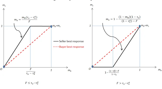
2.2.3 Equilibrium
Combining the analysis above, we can characterize the symmetric equilibrium of the economy using Figure1. There are at least two symmetric pure strategy equilibria. In one of these equilibria,mb =ms = 1: all sellers accept e-money, and all buyers allocate all of their endowment to e-money – call this the all-e-money equilibrium (this equilibrium always exists provided thatF 1 e
s). There is a second symmetric pure strategy equilibrium where
mb =ms = 0and e-money is not accepted by any seller or held by any buyer – call this the all-cash equilibrium. In both equilibria, there is no payment mismatch, and the number of transactions is maximized at1. In the case whereF = s es, there exists a continuum of possible equilibria in whichms 2(0;1)andmb =ms.
The e-money equilibrium is socially optimal as it minimizes total transactions cost. Note that buyers are always better off in the all- e-money equilibrium relative to the all-cash equi-librium. The seller’s relative payoff in the two equilibria, however, depends on the fixed cost,
Figure 1: Symmetric Equilibria
3
Experimental Design
The experiment was designed to match the model as closely as possible, but without the continuum of buyers and sellers of unit mass. Specifically, for each session of our experiment, we recruited 14 inexperienced subjects and randomly divided them up equally between the buyer and seller roles, so that each market had exactly seven buyers and seven sellers. These roles were fixed for the duration of each session to enable subjects to gain experience with a particular role. The subjects then repeatedly played a market game that approximates the model presented in the previous section.
Specifically, subjects participated in a total of 20 markets per session. Each market con-sisted of two stages. The first stage was a payment choice stage. In this first stage, each buyer was endowed with seven experimental money (EM) units (as there were 7 sellers) and these buyers had to decide how to allocate their seven EM between the two payment methods. To avoid any biases due to framing effects, we used neutral language throughout, referring to cash as “payment 1” and e-money as “payment 2”. Thus, in the first stage, buyers allocated their 7 EM between payment 1 and payment 2, with only integer allocation amounts allowed, e.g., 3 EM in the form of payment 1 and 4 EM in the form of payment 2.10 Each seller was endowed with seven units of goods (as there were seven buyers). Sellers were required to accept payment 1 (cash) but had to decide in this first stage whether or not to accept payment
2 (e-money) for that market. Sellers who decided to accept payment 2 had to pay a one-time fixed fee ofT EM per market that enabled them to accept payment 2 in all trading rounds of that market. As explained below,T is related to the fixed costs of adopting the new payment method (F) described in the model and serves as our main experimental treatment variable.
In addition to making payment choices in the first stage, subjects were also asked to fore-cast other participants’ payment choices for that market. We elicited these forefore-casts because we wanted to better understand subjects’ decision-making process and possible feedback ef-fects between buyers and sellers. Specifically, buyers were asked to forecast how many of the seven sellers would choose to accept payment 2 in the forthcoming market. Sellers were asked to supply two forecasts: (1) the average amount of the seven EM units that all seven buyers would allocate to payment 2, and (2) how many of the other six sellers would choose to accept payment 2 in the forthcoming market. These forecasts (or beliefs) were incentivized; subjects earned 0.5 EM per correct forecast in addition to their earnings from buying/selling goods (also in EM). Each seller’s forecast of the average amount of EM that buyers had al-located to payment 2 was counted as correct if it lay within 1of the realized value. The other two forecasts were counted as correct only if they precisely equaled the realized value.11 Note that no participant observed any other sellers’ or buyers’ payment choices or forecasts in this first stage; that is, all first stage choices and forecasts were private information and were made simultaneously.
Following completion of the first stage of each market, play immediately proceeded to the second, “trading” stage of the market, which consisted of a sequence of seven trading rounds. In these seven rounds, each subject anonymously met with each of the seven subjects who was in the opposite role to him/herself, sequentially and in a random order for each market. In each meeting, the buyer and seller tried to trade one unit of good for one unit of payment (recall that the terms of trade in our model are fixed). Specifically, when each buyer met each seller (and not earlier), the buyer learned whether the seller accepted payment 2 or not, and then the buyer alone decided which payment method to use, conditional on the buyer’s remaining balance for that market of either payment 1 or payment 2. Sellers were passive in these trading rounds, simply accepting payment 1 from the buyer or payment 2 if the seller had paid the one-time fee to accept payment 2 in that market, depending on the choice of the buyer. Thus, provided that a buyer had some amount of a payment type that the seller accepted, trade would be successful. For each successful transaction, both parties to the trade earned 1 EM less some transaction costs for the trading round, where the transaction costs
11We chose this incentive scheme in the interest of simplicity as belief elicitation was not the main focus
depended on whether payment 1 or 2 was used, as detailed below.12 Notice that the only instances in which a transaction could not take place (was never successful) were those in which the buyer had only payment 2 and the seller did not accept payment 2. In those cases, no trade could take place and both parties earned 0 EM for the trading round.
Following completion of the seven trading rounds of the second stage of a market, that market was over. Provided that the 20th market had not yet been completed, play then pro-ceeded to a new two-stage market where buyers and sellers had to once again make payment choices and forecasts in the first stage and then engage in seven rounds of trading behavior in the second stage. Buyers were free to change their payment allocations and sellers were free to change their payment 2 acceptance decisions from market to market but only in the first stage of the market; the choices made in this first stage were then in effect for all seven rounds of the second trading stage of the market that followed. Thus, in total there were 20 markets involving seven trading rounds each, or a total 140 trading rounds per session. In each trading round, subjects could earn as much as 1 EM (u = 1) less transaction costs, and in the first stage, they could earn 0.5 EM per correct forecast. Following completion of the 20th market, subjects were paid their cumulative EM earnings from all rounds of all markets at the known and fixed rate of 1 EM = $0.15 and in addition they were paid a $7 show-up payment. Each session lasted for about two hours. The average earnings were between$15
and $25.
To facilitate decision making, we provided subjects with two pieces of information in stage 1, at the same time that buyers were asked to make their payment allocation choices and sellers were asked to make their payment 2 acceptance decisions and both types had to form forecasts as described above. The first piece of information provided to subjects consisted of payoff tables. The buyer’s payoff table reported the buyer’s market earnings if the buyer allocated between 0~7 EM to payment 2 (and his/her remaining EM to payment 1) and if 0~7 sellers accepted payment 2. The seller’s payoff table reported the expected market earnings the seller could get from the two options (accept/reject payment 2) in cases where all buyers choose to allocate between 0~7 EM to payment 2, and where 0~6 of the other
six sellers choose to accept payment 2.13 In addition to these payoff tables, sellers also had
12Note that while buyers were endowed with 7 EM at the start of each market, this endowment had to be allocated between payment 1 and payment 2 for the buyers to actually earn EM in each of the seven trading rounds of the second stage of the market. Buyers could not choose to refuse to engage in trade and redeem their endowment of EM. At the end of each market, unused allocations of EM to either payment method had no redemption value. Further, EM endowments and payments earned in each market were not transferable to subsequent markets. Instead, earnings were recorded and paid out only at the end of the experiment following the completion of the 20th market. Thus, buyers started each new market with exactly 7 EM and had to make payment allocations and payment choices anew in the first stage of each market in order to earn EM in that market.
access to a “what if” calculator that computed their expected earnings in asymmetric cases where the seven buyers made different payment allocation choices. The second piece of information that we provided subjects in stage 1 (beginning with market 2 and every market thereafter) was a history of outcomes in all past markets, including the subject’s payment choice, the number of transactions using each of the two payment methods, the number of no-trade meetings, market earnings from trading, and the number of their correct forecasts. In addition, we reported an aggregate market-level statistic: the number of sellers who had chosen to accept payment 2 in the prior market. We provided the latter information so that sellers could learn about other sellers’ payment 2 acceptance decisions in the just completed market; since all 7 buyers visit all 7 sellers and learn whether each seller accepts payment 2 or not, buyers had this economy-wide piece of information by the end of each market. By providing this same information also to sellers, we made sure that both sides of the market had symmetric information about seller choices.
For simplicity, we set the per transaction cost to be the same for all buyers and sellers, i.e., b = s = = 0:5 for payment 1, and be = es = e = 0:1 for payment 2. Thus, consistent with assumption A1, it was always the case that e = 0:4 in all treatments of our experiment. We also set the utility gained from a sale or purchase, u = 1, so that consistent with assumption A2, u > 0. Our only treatment variable was the once-per-market fixed cost,T, that each seller had to pay to accept payment 2, which corresponds to the parameter F in the model with a continuum of agents via the transformationT = 7F. We initially chose three different values for this main treatment variable: T = 1:6,2:8, and
3:5, respectively.14 Later, in section 6 we consider a fourth value for this treatment variable,
T = 4:5.
Note that, given the lower transaction cost from using e-money, buyers are always bet-ter off in the all-e-money (all-payment-2) equilibrium relative to the all-cash (all-payment-1) equilibrium. However, sellers’ relative payoffs depend on the fixed cost,T. IfT <7( e), as in ourT = 1:6treatment (and represented graphically in the left panel of Figure 1), then the seller’s payoff (like the buyer’s payoff) is higher in the all-e-money equilibrium than in the all-cash equilibrium. IfT > 7( e), as in our T = 3:5 treatment (and represented graphically in the right panel of Figure 1), then the seller’s payoff is lower in the all-e-money equilibrium than in the all-cash equilibrium. Finally, ifT = 7( e), as in ourT = 2:8 treatment, then the seller’s payoffs are the same in both the cash and e-money equilibria. Ta-the sellers.
14The ratio = e= 5and the various values for the fixed cost,T, were chosen to make the transaction and
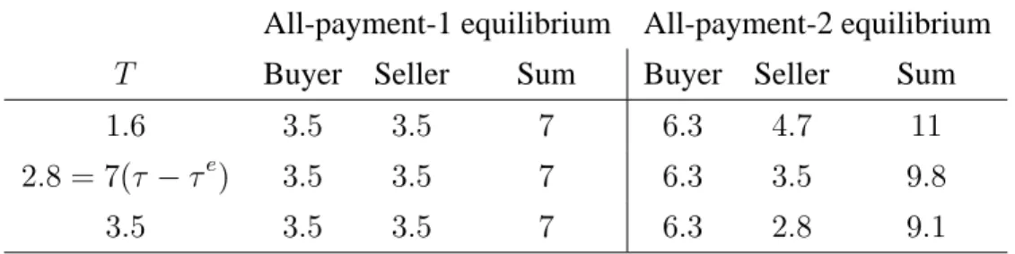
ble 1 reports the net payoffs (in EM) per market, that buyers and sellers earn in the two pure strategy equilibria of each treatment. As this table reveals, the sum of buyers and sellers’ net (of transaction cost) payoffs is always greater in the all-payment-2 equilibrium as com-pared with the all-payment-1 equilibrium so that the all-payment-2 equilibrium is always the socially optimal equilibrium.
Table 1: Payoffs
All-payment-1 equilibrium All-payment-2 equilibrium
T Buyer Seller Sum Buyer Seller Sum
1:6 3:5 3:5 7 6:3 4:7 11 2:8 = 7( e) 3:5 3:5 7 6:3 3:5 9:8 3:5 3:5 3:5 7 6:3 2:8 9:1
In terms of theoretical predictions, under all of our different treatment conditions, there always exist two symmetric pure strategy Nash equilibria, one in which no seller accepts
pay-ment 2 and all buyers allocate all of their endowpay-ment to paypay-ment 1 (the all-cash equilibrium) and another such equilibrium in which all sellers accept payment 2 and all buyers allocate all of their endowment to payment 2 (the all-e-money or card equilibrium). Given our para-meterization, the symmetric payment 2 equilibrium is always the one that maximizes social welfare.
While our focus is on symmetric equilibria, we note that there may also exist asymmet-ric equilibria where some fraction of sellers accept payment 2 while the remaining fraction
do not, and buyers best respond by adjusting their portfolios of payment 1 and 2 so as to perfectly match this distribution of seller choices. These asymmetric equilibria are always present in theT = 2:8treatment, where T = 7( e). In particular, any outcome where
This multiplicity of equilibrium possibilities motivates our experimental study; equilib-rium selection is clearly an empirical question that our experiment can help to address. We hypothesize that, as the transaction cost to sellers of accepting payment 2 increases from
T = 1:6 toT = 2:8and on up to T = 3:5, coordination on the e-money equilibrium will become less likely and coordination on the all-cash equilibrium will become more likely; however, this remains an empirical question, as both symmetric equilibria always co-exist. In addition, we are interested in understanding the dynamic process of equilibrium selection in terms of the evolution of subjects’ beliefs and choices.
The experiment was computerized and programmed using the z-Tree software (Fischbacher,
2007). At the beginning of each session, each subject was assigned a computer terminal, and written instructions were handed out explaining the payoffs and objectives for both buyers and sellers. See Appendix C for example instructions used in the experiment. The experi-menter read these instructions aloud in an effort to make the rules of the game public knowl-edge. Subjects could ask questions in private and were required to successfully complete a quiz to check their comprehension of the written instructions prior to the start of the first market. Communication among subjects was prohibited during the experiment.
We have four sessions for each of our three original treatment conditions,T = 1:6,T = 2:8andT = 3:5. As each session involved 14 subjects with no prior experience participating in our study, we have data from4 3 14 = 168subjects. The experiment was conducted in two locations: Simon Fraser University (SFU), Burnaby, Canada, and at the University of California, Irvine (UCI), USA, using undergraduate student subjects. Specifically, two sessions of each of our three treatments (one-half of all sessions) were run at SFU and UCI, respectively. Our aim in conducting the experiment at two different locations was to assess whether our results would replicate with different subject pools and experimenters conducting the sessions. Despite our use of these two different subject pools, we did not find significant differences in either buyer or seller behavior across these two locations, as we show later in the paper, enabling us to pool our data from both locations.
4
Aggregate Experimental Results
In this section, we present and discuss our experimental results at the aggregate level. The next section will address individual-level behavior.
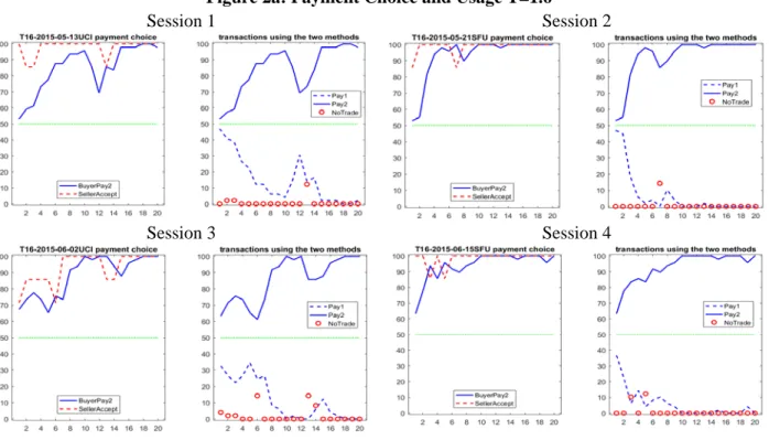
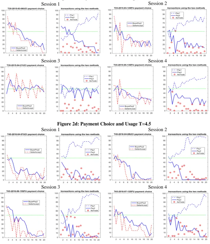
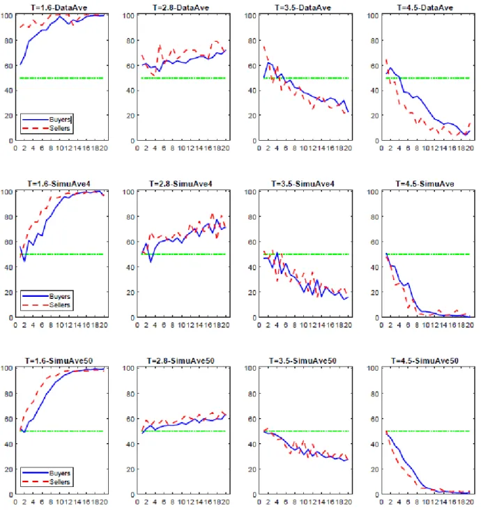
has two panels. In the first (left) panel the series labeled "BuyerPay2," shows the percentage of the buyers’ endowment allocated to payment 2 in each market, averaged across the seven buyers of each session. In this same panel, the percentage of sellers accepting payment 2 in each market is indicated by the series labeled "SellerAccept." The second (right) panel of Figures 2a, 2b and 2c show three time series: (1) the frequency of meetings in each market that resulted in transactions using payment 1 labeled as "Pay1," (2) the frequency of meetings in each market that resulted in transactions using payment 2 labeled as "Pay2," and (3) circles indicating the frequency of no-trade meetings in each market labeled as "NoTrade."
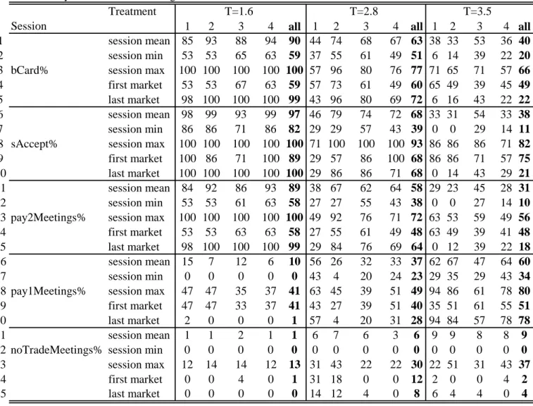
Tables 2 and 3 display various statistics for each of the 12 sessions of the experiment. For each statistic, we show the treatment-level average in bold face. Table 2 provides statistics on five variables that summarize payment choice and usage and transactions. The first part (rows 1 to 10) of Table 2 reports on the percentage of buyers’ endowment allocated to payment 2 averaged across the seven buyers (bCard%) and the percentage of the seven sellers accepting payment 2 (sAccept%). In particular, we report the session mean, minimum and maximum (across the 20 markets), and the value in the first and the last markets of these two statistics. The second part of Table 2 (rows 11 to 25) reports on the percentage of meetings that resulted in trade using payment 2 (pay2Meetings%) trade using payment 1 (pay1Meetings%) or no trade (noTradeMeetings%). Again, we provide the session mean, minimum and maximum, and the value in the first and last markets for these three statistics. Table 3 provides the same set of statistics on payoff efficiency for buyers, sellers or both ("all"), measured as a percentage of the payoffs that could be earned in the all-payment-2 equilibrium (Part 1 of Table 3) and the all-payment-1 equilibrium (Part 2 of Table 3).
We also examine whether there are treatment differences using pairwise Wilcoxon rank-sum tests on data concerning payment choice, usage and efficiency. These results are pre-sented in Table 4. Here we focus on five variables: (1) "bCard%," the percentage of en-dowment allocated to payment 2 averaged across the seven buyers, (2) "sAccept%," the per-centage of the seven sellers accepting payment 2, (3) "pay2Meetings%," the perper-centage of meetings that resulted in trades using payment 2, (4) "Efficiency(all)," the payoffs actually achieved by both buyers and sellers relative to the all-payment-1 equilibrium (status-quo) payoffs, and (5) "No-tradeMeetings%," the percentage of meetings that result in no trade.15 For each of these five variables, we compare the session average and its value in the first mar-ket in treatment 1 versus treatment 2, e.g., T=1.6 versus T=2.8. Each session is treated as an independent observation, so we have four observations on each variable for each treatment.
15For the rank-sum test of efficiency, we use the efficiency measure relative to the payoffs in the
For each pair-wise test, Table 4 reports the rank sums of the two treatments, the z-value and thep-value.
Finally, we test whether a session converges to either of the two symmetric pure strategy equilibria by estimating the process followed by three variables, the percentage of the buyers’ endowment allocated toward payment 2 averaged across the seven buyers (bCard%), the percentage of sellers accepting payment 2 (sAccept%), and the percentage of meetings that resulted in trade using payment 2 (Pay2Meetings%), over time. In particular, we run the following regression for each session and for each of these three variables:
yj;s= jyj;s 1+ j+ j;s; (1)
whereyj;sis the value of the variable being tested in market s for session j. From (1), we say that the variable converges to its payment-1-only equilibrium value if the estimate of the long-run expected value foryj,1 jj, is not significantly different from 0. Similarly, we say that the variable converges to its payment-2-only equilibrium value if j
1 j is not significantly different from100. Table 5 reports the estimates and standard errors for1 j,100 1 jj and
j
1 j. p-values indicate whether the estimated variable is significantly different from0. Thus, if 100 j
1 j (alternatively j
1 j) is not significantly different from zero, then we cannot reject the hypothesis of convergence of that variable to the all–payment-2 (all–payment-1) equilibrium.
Using the data reported in Figures 2a-2c, 3 and Tables 2-5, we summarize results from the aggregate-level analysis of our data as a number of findings.
Finding 1 Across the three treatments, asT is increased from 1:6 to 2:8 to 3:5, there are significant decreases in the buyer’s choice of payment 2, the seller’s acceptance of payment
2, and successful transactions involving payment 2.
Support for Finding 1 comes from Table 4. The rank-sum test results indicate that the buyer’s choice of payment 2 (bCard%), the seller’s acceptance of payment 2 (sAccept%) and successful payment 2 transactions (pay2Meetings%) are significantly higher in theT = 1:6
treatment as compared with either the T = 2:8 or T = 3:5 treatments (p-value< 0:05). Further, these variables are larger in theT = 2:8treatment as compared with the T = 3:5
The next three findings summarize aggregate behavior in each of the three experimental treatments.
Finding 2 WhenT = 1:6, the experimental economies converge to (or nearly converge to) the all-payment-2 equilibrium.
Support for Finding 2 comes from Tables 2 and 5 and Figure 2a, which report on the evolution of behavior in the four sessions of the T = 1:6 treatment. In all four sessions, subjects move over time in the direction of the all payment 2 equilibrium, which in this case represents a strict Pareto improvement for both sides. Furthermore, sellers do not suffer much loss from paying the fixed cost to accept payment 2: they can recover the fee if each buyer allocates just 4 EM (57%) or more to payment 2. As a result, sellers maintain high levels of acceptance, and this steadily high acceptance rate encourages buyers to quickly catch up, which, in turn, reinforces the incentives for acceptance of payment 2. As a result, toward the end of all fourT = 1:6treatment sessions, subjects have achieved convergence or near-convergence to the payment 2 equilibrium. This is also supported by the near-convergence test. As shown in Table 5, the estimated long-run expected values of bCard%, sAccept%, and pay2Meetings%, are not significantly different from 100 for sessions 1, 2 and 4. For session 3, the estimated long-run values of bCard% and pay2Meetings%, are also not significantly different from 100, but the seller’s choice of payment 2, sAccept%, is statistically different from 100, though the magnitude of the difference is small (<5%).
Finding 3 WhenT = 2:8, there is a mixture of outcomes consistent with the greater multi-plicity of equilibria in this treatment.
Support for Finding 3 comes from Tables 2 and 5 and Figure 2b, which report on the evolution of behavior in the four sessions of theT = 2:8treatment. In contrast with theT = 1:6treatment, the data reported in Table 2 and Figure 2b reveal a mixture of outcomes across the four sessions of theT = 2:8treatment. In particular, we observe that the experimental economy either lingers in the middle ground between the 1 and payment-2 equilibria (sessions 1, 3 and 4) or appears to be very slowly converging toward the all-payment-2 equilibrium (session 2).
the fraction of sellers accepting payment 2 hovers above (with some volatility) the fraction of endowment that buyers allocate to payment 2.
If, over time, buyers increasingly insist on the new payment method 2, then sellers are likely to accommodate the buyers’ choices by accepting it; this seems to be the case in session
2. In the final market of session 2of the T=2.8 treatment, we see from Table 2 that buyers’ allocation of their endowment to payment 2 averages 96%, and six out of seven sellers (86%) accept payment 2. The number of payment 2 transactions in this session increases from 55% in the first market to 84% in the last market. The formal convergence analysis (Table 5) suggests that the estimated long-term value of buyer’s choice of payment 2 (bCard%) is not significantly different from 100% in this session. However, the other two variables, seller acceptance rate and percentage of payment 2 meetings, have not yet converged to 100 in a statistical sense. Nevertheless, it seems reasonable to conjecture that session 2 would pass the convergence test if the session had continued beyond 20 markets. Note that, compared with theT = 1:6 treatment sessions, the process of convergence toward the all-payment-2 equilibrium in session 2 of the T = 2:8treatment is considerably slower, more erratic and incomplete.
By contrast, in the other three sessions of theT = 2:8treatment there is little to no ev-idence of convergence toward either the all-payment-1 or all-payment–2 equilibrium. Table 2 reveals that for session 3 there is a small increase in the number of transactions using pay-ment 2 from 61% in the first market to 76% in the final market, but the economy remains far away from the all-payment-2 equilibrium, or any other symmetric equilibrium. In session 1, the number of sellers accepting payment 2 fluctuates between 2/7 (28.5%) and 5/7 (71.4%). Consequently, buyers are not willing to take the lead by acquiring high payment 2 balances, fearing that they will not be able to trade in case some sellers reject payment 2. As a result, the buyer’s average payment 2 allocation and the number of sellers accepting payment 2 both average between 40-50% throughout the entire session, but there is never coordination on the same rate. Finally, session 4 shows an upward trend in payment 2 usage in the first seven markets, but this trend abruptly halts thereafter, with the average number of payment2 trans-actions barely changing from market eight onward (the value fluctuates between 67% and 71%). This outcome represents near (but imperfect) convergence to an interior asymmetric equilibrium where approximately five out of seven sellers are accepting payment 2 and buy-ers are allocating approximately 5 units of their 7 EM endowment to payment 2. This is the closest instance we have to a dual payments equilibrium outcome in our data.
Support for Finding 4 comes from Tables 2 and 5 and Figure 2c, which report on the evolution of behavior in the four sessions of theT = 3:5treatment. WhenT = 3:5, sellers do better in the payment 1 equilibrium as compared with the payment 2 equilibrium; by contrast buyers always prefer the payment 2 equilibrium. Nevertheless, in each of the four sessions, more than 50% of sellers start out in the first market accepting payment 2, perhaps fearing that they will lose business in the case where some buyers show up with only payment 2 remaining. With experience, sellers learn to resist accepting payment 2 and to engage in a “tug-of-war” with buyers; the average acceptance rate over all four sessions declines from 75% in the first market to just 21% in the last market. Sellers appear to be winning this contest in sessions1, 2 and4, pulling the economy back in the direction of the status quo, all-payment-1 equilibrium. For example, in session 1 of the T = 3:5 treatment, Table 2 reveals that buyer’s payment 2 allocation falls from 65% in the first market to an average of just 6% in the last market. On the seller’s side, six out of seven sellers in this session (86%) accept payment 2 in the first market; by the last market of this session, no seller is accepting payment 2. The number of payment 1 transactions increases from 35% in the first market to 94% by the final, 20th market; over the same interval, payment 2 transactions fall from 63% to 0%.
Table 5 reveals that session 1 of theT = 3:5treatment passes the formal convergence test, with all three variables bCard%, sAccept% and pay2Meetings% not statistically different from 0.16 In sessions 2 and 4 of the T = 3:5 treatment, the trend works in favor of the seller, but the speed of convergence is slow; at the end of the session 2(4), 12% (22%) of transactions are still conducted in payment 2. Sessions 2 and 4 do not pass the convergence test; however, given the downward trend in payment 2 choice and usage, one can reasonably conjecture that convergence to the all-payment-1 equilibrium would be achieved with more market repetitions. In session3, the tug of war continues throughout the session and neither side is able to gain the upper hand; in that session, the average buyer’s payment 2 allocation and the number of sellers accepting payment 2 consistently fluctuates around 50%, but there is no coordination on any asymmetric equilibria in this setting. This session does not pass the convergence test either and it is not clear whether the session would converge even with more market repetitions.
An immediate implication of Findings 1 to 4 is the following:
Finding 5 Efficiency losses increase with increases inT.
Support for Finding 5 comes from Tables 3 and 4. WhenT = 1:6, the economy quickly
16The estimate of the long-run equilibrium value of bCard% is negative from the unconstrained estimation,
converges to the socially efficient all–payment–2 equilibrium. All four sessions achieve be-tween 92% and 96% of the socially optimal (payment-2-only) equilibrium payoffs, with the overall average being 94%. The efficiency measure falls asT increases to2:8, ranging from
75%to85%, with a treatment average of81%. TreatmentT = 3:5induces a further decrease in the efficiency measure, which now ranges from 72% to 75% and has a treatment average of 75%. As the fixed cost increases, the economy moves further away from the efficient equilibrium. At the same time, mis-coordination in payment choices becomes more severe, as manifested in the increasing frequency of no-trade meetings, which averaged 0:8% for
T = 1:6,5:6%forT = 2:8and8:6%forT = 3:5.
The picture is unchanged if we consider earnings relative to the status quo where only payment 1 is used. The percentage of subjects’ earnings relative to the payment 1 equilibrium level serves as a measure of the benefit of introducing the new payment method, payment 2. As revealed in the bottom half of Table 3, there are significant positive welfare benefits to the introduction of payment 2 whenT = 1:6, moderate benefits whenT = 2:8, but almost no benefit whenT = 3:5. The treatment differences in efficiency and no-trade meetings are also statistically significant as shown by the rank-sum tests in Table 4. Disaggregating by role, Table 3 further reveals that in all three treatments, buyers benefit relative to the all-payment-1 equilibrium, while sellers only benefit in theT = 1:6treatment and sellers suffer in the other two treatments relative to the all payment 1 equilibrium benchmark. The latter finding is summarized as follows.
Finding 6 Sellers may choose to accept the new payment method (payment 2) even if doing
so reduces their payoffs relative to the status quo where only payment 1 is used.
Merchants often complain about high costs associated with accepting electronic payments but feel obliged to accept those costly payments for fear of upsetting or losing their customers (the so-called "must-take" phenomenon). A recent study by Bounie, François and Van Hove (2017) finds that in the case of France in 2008, the must-take phenomenon applies to 5.8-19.8% of card-accepting merchants.17 We observe a similar pattern in our experiment. For instance, when T = 3:5, although sellers understand that they will lose relative to the sta-tus quo if the economy moves to the all-payment-2 equilibrium, most sellers still begin the session accepting the new payment method (the average frequency of sellers accepting pay-ment 2 in the first market is 70% in treatpay-ment T = 2:8 and 76% in treatment T = 3:5).
Furthermore, in all sessions with T = 2:8 and 3:5, throughout all 20 markets, the seller’s average payoff is always below3:5, the payoff that they would earn if the economy were in the all-payment-1 equilibrium.18
5
Individual Experimental Results
In this section we explore in further detail individual decision-making in our experiment. In particular, we examine the buyers’ portfolio decisions and the sellers’ payment 2 accep-tance decisions taking into account treatment variables and buyers and sellers’ elicited beliefs. Since the impact of beliefs on behavior can result in endogeneity issues, we adopt an instru-mental variables (IV) regression approach.19 In the first stage, we regress the individual’s belief concerning the other players’ payment choices for the current market on the outcomes that obtained in the previous market, together with four control variables: the market number, 1,2...20 ("market") to capture any time trend, a location dummy ("location") equal to 1 if the data were collected at SFU, and two treatment dummies, T16 and T35, to pick up treatment level effects from theT = 1:6andT = 3:5treatments respectively (the baseline treatment is thusT = 2:8). In the second stage, we regress the payment choice on the estimated belief term and the control variables. The specific rationale for this two-stage regression is that individuals’ payment choices depend on their beliefs about other players’ choices, and their beliefs are in turn affected by historic outcomes.
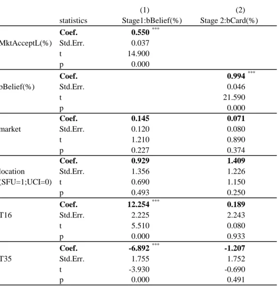
Table 6 reports regression estimates for the buyer’s decision.20 The first-stage regression is a linear, random effects regression model of buyer’s beliefs. The dependent variable is "bBelief%", the buyer’s own incentivized belief as to the number of sellers who would be ac-cepting payment 2 in the current market. The main independent variable is "mktAcceptL%," representing the percentage of sellers accepting payment 2 in the last market.21 In addition, there are four control variables: market, location, T16 and T35. The second-stage regression is a linear, random effects regression model of the buyer’s portfolio decision. The dependent variable is the percentage of the buyer’s endowment that he/she allocated to payment 2 (card
18See Figures Ab and Ac in Appendix A.
19Each regression has 1596=12x7x19 observations. There are 12 sessions (four sessions for each of the three
treatments), each with 7 buyers or sellers and 20 markets. There are 19 observations for each individual as the first-stage regression involves lagged variables in the past market, so the first market has to be excluded. The regressions have clustered errors at the individual subject level.
20The regressions were carried out using the Stata command xtivreg.
choice%), and the explanatory variables are the estimated bBelief% term from the first stage and the four control variables.22
In the first-stage regression, the coefficient on MktAcceptL(%) is positive and statistically significant with ap-value close to zero, which suggests that buyers adjust upward their belief about seller acceptance of payment 2 in the current market after observing a higher past market seller acceptance of payment 2. Compared with the baseline treatmentT = 2:8, the buyer’s belief about seller acceptance of payment 2 is 12% higher in treatmentT = 1:6, and
7% lower in treatmentT = 3:5; both coefficients are statistically significant withp-values close to zero. There is no significant time trend in buyer’s belief (the variable market is insignificant). The location dummy variable is also insignificant, suggesting that there was no significant difference in buyers’ beliefs between SFU and UCI.
In the second-stage regression, only the coefficient on bBelief(%) is significant. The coefficient on bBelief(%) is 0.994, which is very close to 1. This finding is consistent with the theory: the buyer’s best response is to allocatex%of their endowment to payment 2 if they expectx%of sellers to accept payment 2. We summarize these results as follows.
Finding 7 Buyers’ portfolio choices depend on their beliefs about sellers’ acceptance of
payment 2, and these beliefs in turn depend on historic market outcomes and the value ofT.
Table 7 reports regression estimates from the seller’s acceptance decisions. Again, we used an IV regression, for the same reasons given for buyer choices. The first stage estimates the sellers’ beliefs concerning other sellers’ acceptance decisions and about buyers’ portfolio choices using linear, random-effects models. The dependent variables are "sBeliefB(%)" and "sBeliefS(%)," which are the seller’s incentivized beliefs about the buyers’ average alloca-tion of their endowment to payment 2 and the percentage of the other six sellers (excluding themselves) who would accept payment 2, respectively, in the current market. For the inde-pendent variables, besides the four control variables used in the regression on buyer payment choices, there are four variables that capture the historical data: "sOtherAcceptL(%)," which is the percentage of sellers who accepted payment 2 in the previous market (this historical information was only revealed to sellers at the start of stage 1 of each new market when they had to make a payment 2 acceptance choice and not earlier); "sAcceptL," which is the seller’s own acceptance decision in the previous market; "sCardDealL(%)," which is the percentage of transactions the seller succeeded in conducting using payment 2 in the previous market;
22In the context of the payment choice game, the buyer’s payoff depends on his/her own portfolio choice and
and "sNoDealL(%)," which is the percentage of no trade outcomes the seller encountered in the previous market. The second-stage regression is a probit, random-effects model of the seller’s acceptance decision. The dependent variable, "sAccept," is a binary variable, which is equal to 1 if the seller accepts payment 2, and 0 otherwise. The explanatory variables are the estimated belief terms from the first-stage regression, sBeliefB(%) and sBeliefS(%), and the four control variables. For the second-stage regression, Table 7 shows the marginal effects of the explanatory variables on the seller’s probability (in %) of accepting payment 2. From the first column in Table 7, we see that sellers adjust their beliefs about buyers’ al-location of their endowments to payment 2 upward if the sellers completed more payment-2 transactions (sCardDealL(%)) or encountered more no-trade meetings (sNoDealL(%) in the previous market. This result is intuitive. If the seller accepted payment 2 in the previous mar-ket, then more payment-2 meetings imply that buyers carry higher payment-2 balances. If the seller did not accept payment 2 in the previous section, then more no-trade meetings also im-ply that buyers have higher payment-2 balances. In either case, the seller adjusts sBeliefB(%) upward. The negative coefficient before sAcceptL means that the sBeliefB(%) term for sell-ers who accepted payment 2 in the previous market has a lower intercept as compared with those who did not accept payment 2 in the previous market. The positive coefficient before sOtherAcceptL(%) suggests that sellers expect buyers to increase their payment 2 balances after observing a higher market acceptance rate for payment 2 in the previous market. The coefficient of the location dummy is small in magnitude and is not statistically significant. There is no significant time trend in sBeliefB(%) as indicated by the insignificance of the market number variable. The coefficients on the two treatment dummies have the expected signs (positive for T16 and negative for T35), but are not statistically significant at the 10% significance level.
Sellers’ beliefs about other sellers’ payment 2 acceptance choices follow a similar pattern to their beliefs about buyers’ allocation of endowments to payment 2. As the second column of Table 7 reveals, sellers expect the fraction of other sellers accepting payment 2 to increase if they completed more payment 2 transactions or encountered more no-trade meetings: they expect other sellers to respond to buyers’ higher payment 2 balances in the previous market. They also expect the higher acceptance rate in the previous market to persist into the current market (the coefficient on sOtherAcceptL% is 0.457 and the p-value is close to 0). The treatment dummies have the same signs as in the regression for sellers’ beliefs about buyers’ portfolio choices, but are statistically significant (thep-value is 0.030 for T16 and 0.054 for T35). Sellers’ beliefs about other sellers do not exhibit significant time trend or location effects.
crucially on their beliefs about buyers’ portfolio choice. In the second-stage regression, the coefficient on sBeliefB(%) is 1.008 and has ap-value close to 0. In words, the probability of a seller accepting payment 2 increases by 1% if they expect buyers to increase their allocation to payment 2 by 1%. The effect of sellers’ beliefs about other sellers’ payment 2 acceptance decisions is small in magnitude and not statistically significant. Thus it is principally sellers’ beliefs about buyer behavior that matter most for their acceptance decisions. The treatment effects have the expected signs; relative to the T = 2:8 treatment, the sellers’ acceptance rate is more than 15% higher in treatmentT = 1:6, and the difference is significant at the 10% level. There is again an absence of any significant time trend or location effect. We summarize our findings for seller behavior as follows:
Finding 8 Sellers’ acceptance of payment 2 depends onT and on sellers’ beliefs about buyer allocations to payment 2; these beliefs, in turn, depend on historic market outcomes.
Summarizing the IV regression results, we have found that both buyers and sellers adjust their behavior in a manner that is consistent with our theory. Buyers’ portfolio choices de-pend crucially on their beliefs about sellers’ acceptance decisions, and, vice versa, sellers’ acceptance decisions depend crucially on their beliefs about buyers’ portfolio choices, sug-gesting that the payment choice in our experiment exhibits a strong network effect.23 The payment system evolves over time as subjects adjust their beliefs, and therefore their choices, in response to historic data. We have also confirmed the strong treatment effects (either di-rectly on choices or indidi-rectly through beliefs) that we report on earlier in finding 1. Finally, we have not found evidence for any strong location effects in the decisions made by buyers or sellers, despite the fact that we conducted our experiment using student subjects at two different universities, SFU and UCI.
6
An Evolutionary Learning Model of Payment Choice
While our theoretical model is static, the adoption of a payment method is inherently a dynamic process. Our experiment suggests that this dynamic process involves some learn-ing over the repeated markets of our design. Toward a better understandlearn-ing of this dynamic learning process, in this section we present an evolutionary learning model approach to pay-ment choice and compare simulation results using that model with our experipay-mental data. After establishing that our evolutionary model provides a good fit to our experimental data, we use the model to predict outcomes for a fourth experimental treatment. That is, we use the evolutionary model for experimental design. We then carry out an additional experimental treatment and again find a good fit between the evolutionary model and this new experimental data.
6.1
The IEL Model
The evolutionary learning model we use is the individual evolutionary model (IEL). That model has been successfully used to characterize and predict the behavior of human subjects in many different economic environments (see, for example, Arifovic and Ledyard, 2007, 2011, 2012, 2018; Arifovic, Boitnott and Duffy, 2019).
In this model, each individual agent is endowed with a set ofJ strategies. This collection of strategies is updated each period based on evaluation of agent i’s foregone payoff from using each strategy, i.e., how each strategy would have performed had it been used in that period. Strategies with higher foregone payoffs increase the frequency of their representation in each agent’s strategy set. Finally, there is a probability of experimentation, which brings new strategies into the set. The strategy that is actually used by each agent in a given period is selected randomly, where the probability of selection is proportional to a strategy’s relative foregone payoff among the strategies in the agent’s set.
The environment in which we simulate the IEL model corresponds precisely to our exper-imental environment, i.e., it is inhabited by seven buyers and seven sellers, and it lasts for 20 markets (periods) with each period involving a first payment choice stage followed by a sec-ond stage of seven trading rounds. The sequence of events in each period and round exactly follows the experimental design. The artificial agents have the same amount of information that the human subjects had at every decision node.
Each of the seven artificial buyers and sellers in our evolutionary model has as a set of
f0;1; :::;7g, where j 2 f1;2; :::; Jg, represents the number of EM units the buyer places in payment 2 in market (period) t.24 For seller i 2 f1;2; :::;7g, a rule mi
s;j(t) 2 [0;1], wherej 2 f1;2; :::; Jg, represents the probability that the seller accepts payment 2. When a particular seller rule is selected as an actual rule, a random number between0and1is drawn from a uniform distribution over [0;1]. If that number is less than or equal to mi
s;j(t), the seller decides to accept payment2. Otherwise, the seller decides not to accept payment 2 for that market.
The initial set ofJ rules (strategies) for all buyers and sellers is randomly chosen. Then, for the initial market, one strategy is randomly chosen for each buyer and each seller from their initial set ofJ strategies and those are the strategies played in the first market. There-after, the updating of the buyers’ and sellers’ sets of rules and the strategy chosen by each player takes place at the end of each seven-round market and consists of four steps:
1. Experimentation. Experimentation introduces new, alternative rules that otherwise might never have a chance to be tried. It ensures that a certain amount of diversity is maintained. This operation involves changing each element of the current set of rules to a new rule with some probability, t. The new rule is drawn from a normal distribution, with mean equal to the current rule and standard deviation equal to t.25 Both tand tdecay exponentially over time. Further details are provided in Appendix B.
2. Foregone payoff calculation. As the rules that our IEL sellers and buyers use are simple, the foregone payoff calculation is what gives the algorithm its power. The foregone payoff calculation depends on whether an agent is a buyer or a seller.
At the end of each period, buyers know the number of sellers who actually accepted payment 2 in that period,sa(t)2 f0;1; :::;7g. For buyers, the foregone payoff of each rulemi
b;j(t)in buyeri’s set at the end of markettis computed in the following way. i
b;j(t) = (7 m i
b;j(t))(u ) + min sa(t); mib;j(t) (u e):
Note that in our simulation, we assume that the buyer adopts the following (payoff-maximizing) strategy (given her initial payment allocation): if the buyer meets a seller who accepts payment 2, then the buyer uses payment 2 if he still has payment 2 left and she uses payment 1 otherwise; if the seller does not accept payment 2, then the buyer
24To be precise, the buyer’s rule is a real number between 0 and 7, which is rounded to the nearest integer if the rule is selected.
25If the draw from the normal distribution is larger (smaller) than the upper (lower) limit of the choice set,