W
HEN THEH
ONEYMOON ISO
VER:
T
HEE
FFECTS OFF
AMILYS
TRUCTUREON
C
HILDREN’
SC
OGNITIVE ANDN
ON-
COGNITIVEA
CHIEVEMENTSNing Fu
A dissertation submitted to the faculty of the University of North Carolina at Chapel Hill in par-tial fulfillment of the requirements for the degree of Doctor of Philosophy in the Department of
Economics.
Chapel Hill 2017
Approved by:
Donna B. Gilleskie
Luca Flabbi
Jane Cooley Fruehwirth
David K. Guilkey
c 2017 Ning Fu
ABSTRACT
NING FU: When the Honeymoon is Over: The Effects of Family Structure
on Children’s Cognitive and Non-cognitive Achievements. (Under the direction of Donna B. Gilleskie)
This dissertation examines the effects of family structure on children’s cognitive and
non-cognitive achievements, using data on females and their children from the 1979 cohort of the
National Longitudinal Survey of Youth. To deal with dynamic selection into married, cohabiting
or single households, I model women’s relationship status, school enrollment, employment, family
size, and investment in children over the life cycle. All of these behaviors, and the production of
children’s achievements, are estimated using a random effects joint estimation procedure, which
allows the unobserved heterogeneity of the woman and her children to influence both maternal
be-haviors and children’s outcomes. I find that, compared to growing up in single households, being
born and raised in married households significantly decreases children’s behavioral problems by
0.17 to 0.28 standard deviations, depending on the child’s age and gender. These gains are
ex-hibited by children under age ten. Moreover, compared to being raised in cohabiting households,
growing up in continuously married households decreases girls’ behavioral problems by 0.4
stan-dard deviations, during ages four to six. In addition to measuring causal marginal effects of family
structure, this dissertation uses simulation to evaluate how various policy interventions, including
marriage promotion, maternal education promotion, and parenting skills training, could potentially
ACKNOWLEDGMENTS
Firstly, I would like to express my sincere gratitude to my advisor Donna B. Gilleskie for her
invaluable guidance, encouragement and support. The passion and rigor she brings to research are
highly contagious and motivating, and her expertise and understanding have always kept my hopes
up through tough times in my Ph.D. pursuit. Above all, I am thankful for the wonderful example
she has set about how to be loving and compassionate as a person. It has been an honor to be her
student, and I could not have imagined having a better advisor and mentor.
I would also like to thank my thesis committee members, Luca Flabbi, Jane Cooley Fruehwirth,
David K. Guilkey, and Helen V. Tauchen, for their continuous contributions of time, ideas, and
guidance. I am fortunate to have a committee that not only raise deep questions for my research,
but also go far and beyond in guiding me to answer them. Their immense knowledge, constructive
comments, and warm encouragement have greatly improved not only the quality of my research,
but also my overall experience as a Ph.D. student. I am also grateful for the guidance I received
from Klara S. Peter when I was a predoc trainee at the Carolina Population Center. She held
my hand through my first Ph.D. research project, and her diligence to research has been a great
inspiration for me throughout my Ph.D. study.
I thank Raquel Bernal, Hanming Fang and Michael P. Keane for generously sharing their data
on U.S. welfare policies. I am also grateful for the Robert Gallman Scholarship, the Williamson
Family Fund, the Mathematica Research Policy Summer Research Fellowship, and the Dissertation
Completion Fellowship for their generous support for my research.
My sincere thanks also goes to my colleagues at UNC, who have been providing friendship,
insightful comments, and moral support throughout my Ph.D. study. The highly collegial
environ-ment in the departenviron-ment has made the Ph.D. study so much more fun.
Lastly, a special thanks to my parents and my husband. Their love and support have always
TABLE OF CONTENTS
LIST OF TABLES . . . vii
LIST OF FIGURES . . . ix
1 Introduction . . . 1
2 Related Literature . . . 4
2.1 Family Structure is Not Random . . . 4
2.2 Production of Children’s Cognitive and Non-cognitive Achievements . . . 5
3 Empirical Framework . . . 8
3.1 Timing and Notation . . . 8
3.2 Estimable Structural Equations and Production Functions . . . 12
3.3 Attrition and Initial Condition Equations . . . 15
3.4 Likelihood Function . . . 17
3.5 Identification . . . 17
4 Data . . . 19
4.1 Description of Key Variables . . . 25
4.2 Exogenous Prices and Supply-side Variables . . . 28
5 Estimation Results . . . 29
5.1 Replication of Previous Literature . . . 29
5.2 Results from the Dynamic Dynamic Multiple-equation Model . . . 31
5.2.1 Model Fit . . . 31
5.2.3 Estimates of the Contemporaneous and Life-cycle Marginal Effects . . . . 33
6 Policy Experiments . . . 39
6.1 Experiment A - Marriage Promotion . . . 39
6.2 Experiment B - Maternal Education Promotion . . . 41
6.3 Experiment C - Parental Investment Increase . . . 45
7 Conclusion . . . 47
A NLSY79-Child HOME-SF Scales and Joint Estimation Results . . . 48
LIST OF TABLES
3.1 Specification Summary for Jointly Estimated Set of Equations . . . 16
4.1 Empirical Distribution of Research Sample . . . 20
4.2 Descriptive Statistics for Dependent Variables . . . 21
4.3 Descriptive Statistics for Endogenous Individual Explanatory Variables . . . 22
4.4 Descriptive Statistics for Exogenous Individual Explanatory Variables . . . 23
4.5 Descriptive Statistics for Exogenous Price and Supply-Side Variables . . . 24
5.1 Alternative Specifications of Achievement Production Functions . . . 31
5.2 Summary Statistics for Model Fit . . . 32
5.3 Contemporaneous Marginal Effects of Family Structure on Child Achievements . . 34
5.4 Life-cycle Marginal Effects of Family Structure on Boys’ PIAT Math Percentile Score by Age . . . 35
5.5 Life-cycle Marginal Effects of Family Structure on Girls’ PIAT Math Percentile Score by Age . . . 36
5.6 Life-cycle Marginal Effects of Family Structure on Boys’ Behavioral Problem Per-centile Score by Age . . . 37
5.7 Life-cycle Marginal Effects of Family Structure on Girls’ Behavioral Problem Per-centile Score by Age . . . 38
6.1 Experiment A1 - Effects of Marriage Promotion on Child Achievements with 50% Success Rate . . . 40
6.2 Experiment A2 - Effects of Marriage Promotion on Child Achievements with 100% Success Rate . . . 41
6.3 Experiment B1 - Effects of Education Promotion on Child Achievements with 50% Success Rate . . . 43
6.4 Experiment B2 - Effects of Education Promotion on Child Achievements with 100% Success Rate . . . 44
6.6 Experiment C2 - Effects of Parental Investment Increase (by 30 percentage points)
on Child Achievements . . . 46
A.1 NLSY79-Child HOME-SF Scales for Children under age 3 . . . 48
A.2 NLSY79-Child HOME-SF Scales for Children age 3-5 years . . . 49
A.3 NLSY79-Child HOME-SF Scales for Children age 6-9 years . . . 50
A.4 NLSY79-Child HOME-SF Scales for Children age 10-14 years . . . 51
A.5 Estimation Results: Relationship Status (cohabiting relative to married) . . . 52
A.6 Estimation Results: Relationship Status (single relative to married) . . . 53
A.7 Estimation Results: School Enrollment (enrolled relative to not enrolled) . . . 54
A.8 Estimation Results: Employment Status (full-year part-time employed relative to full-year full-time) . . . 55
A.9 Estimation Results: Employment Status (part-year full-time employed relative to full-year full-time employed) . . . 56
A.10 Estimation Results: Employment Status (part-year part-time employed relative to full-year full-time employed) . . . 57
A.11 Estimation Results: Employment status (unemployed relative to full-year full-time employed) . . . 58
A.12 Estimation Results: Employment status (out of labor force relative to year full-time employed) . . . 59
A.13 Estimation Results: Family Size Change (gain any children relative to no change) . 60 A.14 Estimation Results: Family Size Change (lose any children relative to no change) . 61 A.15 Estimation Results: Investment in Child . . . 62
A.16 Estimation Results: Log Wage . . . 63
A.17 Estimation Results: Log of Spouse/Partner Income . . . 64
A.18 Estimation Results: Child PIAT Math Percentile Score . . . 65
LIST OF FIGURES
3.1 Timeline . . . 10
4.1 Family Structure Probabilities at Age t . . . 26
4.2 Comparisons of Behavior Probabilities by Family Structure . . . 26
CHAPTER 1
INTRODUCTION
The United States has experienced dramatic changes in family structure since the 1960s. In
2014, over 40 percent of births were to unmarried women, up from only 5.3 percent in 1960.1
Data indicate that children growing up in single or cohabiting households have less education,
worse health outcomes, and lower future marriage and socioeconomic prospects (e.g., McLanahan
and Sandefur, 1994; Buchanan, Maccoby, and Dornbusch, 1996; Ermisch and Francesconi, 2001;
Manning and Lamb, 2003; Brown, 2004; Amato, 2005). Intended to reduce single parenthood and
improve children’s welfare, the federal government has been providing $150 million each year
since 2005 to support the Healthy Marriage and Responsible Fatherhood Initiative based, in part,
on these observed correlations. However, in order to design effective evidence-based policy, it
is essential to realize that the frequently-cited correlations between non-marital parenthood and
children’s adverse outcomes do not necessarily imply a causal relationship. Using the National
Longitudinal Survey of Youth 1979, this dissertation measures the causal impacts of family
struc-ture on school-aged children’s cognitive and non-cognitive achievements.2
With the goal of uncovering causal relationships, this dissertation develops and estimates a
dynamic, multiple-equation model to explain women’s simultaneous behaviors over the life cycle
regarding their relationship status, school enrollment, employment, family size and investment in
children, and to empirically evaluate how the observed behaviors influence children’s cognitive and
non-cognitive achievements. When making decisions each period, women take into account their
histories of relationships, schooling, employment, family size, and children’s past achievements.
1Statistics are from Child Trends Data Bank (2015).
Their behaviors are also affected by demographic characteristics of the household and the
time-varying state and local environment. These decisions could change across periods as circumstances
evolve, such as the accumulation of work experience, aging of the woman and her children, or
fluctuations in local unemployment rates. A woman’s behaviors, her child’s past cognitive and
non-cognitive achievements, and the unobserved characteristics of the mother and of the child
jointly determine each child’s achievements in each period.
Compared with the existing literature that explores causal effects of family structure on
chil-dren’s outcomes, this dissertation stands out in three ways. First, it establishes the unbiased causal
impacts of family structure on children’s achievements, while jointly considering other life-cycle
decisions, such as employment and fertility, all of which could impact children’s achievements.
Current causal studies focus on the endogeneity of only one behavior, namely family structure,
treating related behaviors as exogenous. Failing to model jointly-made decisions that may be
cor-related with unobservables may produce biased effects of family structure on children’s
achieve-ments. In this dissertation, I jointly model the dynamics of relationship status, as well as other
major life-cycle behaviors and children’s achievements, allowing all these dynamic behaviors and
outcomes to influence each other, as well as be influenced by exogenous characteristics,
unob-served correlated heterogeneity and random shocks.
Second, this dissertation examines the impacts of family structure on children who have never
experienced family structure changes. The fixed-effects approach, which is commonly used in
the literature to address the endogeneity of family structure, relies on either differences in family
structure experience across siblings in the same household (i.e., the household fixed effects), or
changes in family structure a child experiences over time (i.e., the child fixed effects). The effects
identified from such transition households cannot be used to infer the effects of family structure
on children who are born and raised in always single/cohabiting/married households. The joint
estimation approach used in this dissertation enables me to identify and compare the latter effects.
Specifically, I find that, compared to growing up in continuously single households, being born and
by 0.17 to 0.28 standard deviations, depending on the child’s age and gender. These beneficial
im-pacts are statistically significant for children under age 10. Moreover, compared to being raised in
cohabiting households, growing up in continuously married households decreases girls’ behavioral
problems by 0.4 standard deviations, during ages 4 to 6.
Third, I evaluate the potential impacts of alternative policy interventions that aim to change
different aspects of women’s behaviors, and I establish bounds for such effects. The literature on
the production of children’s cognitive and non-cognitive achievements has explored the impacts
of existing policies or natural experiments. However, without modeling individuals’ dynamic
be-haviors, these papers are not equipped to examine how children’s outcomes would differ under
alternative intervention scenarios. For example, if a marriage intervention program does not
af-fect participants’ propensity to get married, policy evaluation studies cannot infer how children’s
achievements would have changed if the program was effective in changing marriage rates. In
addition, evaluations of a marriage intervention program are not able to answer broader questions
about the potential impacts of an intervention on the target population that improves a mother’s
education level instead of promoting marriage. Through estimation and simulation of channels of
influence on children’s outcomes, this dissertation can answer both types of questions. Specifically,
I find that effective marriage promotion programs have the potential to produce small, favorable
impacts on children’s behavioral problems for initially single households. Interventions that
suc-cessfully encourage unmarried mothers to continue their education and interventions that increase
CHAPTER 2
RELATED LITERATURE
2.1 Family Structure is Not Random
The difficulty in measuring the effects of family structure on children’s outcomes stems from
the nonrandomness of family structure. Specifically, observed and unobserved characteristics of
the parent(s) and of the child may be correlated with both the observed family structure and the
child outcomes. Researchers have used two approaches to address this endogeneity of family
structure. The first approach uses within-family (across siblings) or within-child (at different ages)
fixed effects (Aughinbaugh, Pierret, and Rothstein, 2005; Gennetian, 2005; Bj¨orklund, Ginther,
and Sundstr¨om, 2007; Cooper, Osborne, Beck, and McLanahan, 2011). It is worth noting that
the fixed-effect approach can only eliminate invariant unobserved characteristics. It fails to
cap-ture time-varying determinants that jointly influence family struccap-ture and child achievements. For
example, suppose a mother recently lost her job. On the one hand, this event could worsen the
relationship with her husband and eventually lead to a divorce and, on the other hand, it could
neg-atively impact her child’s achievements since she might alter investment in the child due to the job
loss. Fixed-effects analysis would fail to capture the changes in employment and parental
invest-ments (if not modeled), and lead to the potentially incorrect conclusion that the family structure
change causally decreases children’s achievements. In this dissertation, several mechanisms are
jointly modeled as endogenous dynamic life-cycle behaviors that may affect child development.
These include relationship, schooling, employment, family size, and investment in children.
The second approach that has been used in the literature to address the potentially
nonran-dom nature of family structure includes families that experience a parental death to serve as an
assumption that a parental death is exogenous to other child development inputs or child
develop-ment itself is questionable. As McLanahan, Tach, and Schneider (2013) point out, deaths related to
violence or accidents may reflect selection into risky behaviors, and illness-related deaths may
re-flect selection into particular lifestyles (such as smoking and drinking) or genetic endowment that
may also affect child outcomes. Biblarz and Gottainer (2000), for example, find that, compared
with children raised in single-mother families created by the death of the father, children raised in
divorced single-mother families have significantly lower levels of education, occupational status,
and happiness in adulthood. Corak (2001) finds that, relative to children from intact families,
chil-dren whose parents divorced postpone marriage and they are more likely to suffer separation or
divorce once married. Children from bereaved families, on the other hand, are no different in their
marital behavior than those from intact families. As such, the measured effect of parental
disso-lution associated with a parental death cannot be expanded to that of divorced or selected single
parenthood.
To better understand why and how family structure is determined, a number of studies use
dynamic structural models to explicitly model the decision making process of forward-looking
individuals with regard to marriage, cohabitation and divorce, along with other life-cycle decisions
such as employment and schooling (Brien, Lillard, and Stern, 2006; Keane and Wolpin, 2010;
Laufer and Gemici, 2011; Blau and van der Klaauw, 2013; Flabbi and Flinn, 2015). These papers
provide a theoretical framework to make explicit how different life-cycle decisions are correlated
and jointly determined, and to derive the demand functions used in this dissertation. Given the
focus on children’s outcomes, this dissertation includes parental investment as an endogenous
time-varying behavior that is not commonly modeled in this literature. It also allows a woman’s behavior
to be influenced by her children’s past cognitive and non-cognitive achievements.
2.2 Production of Children’s Cognitive and Non-cognitive Achievements
This dissertation relates to the literature on the production of school-aged children’s cognitive
literature: the policy effect and the productive effects of inputs.1 The policy effect identifies the
average or total effect of an intervention on achievements without controlling for other possible
inputs. This effect is estimated using experiments such as the Tennessee Student/Teacher
Achieve-ment Ratio (STAR) experiAchieve-ment (Finn and Achilles, 1990; Mosteller, 1995; Krueger, 1998, 2003;
Fryer, Levitt, and List, 2015; Mayer, Kalil, Oreopoulos, and Gallegos, 2015), or natural
experi-ments such as welfare reform and state-level policy changes (e.g., Bernal and Keane, 2011; Juhn,
Rubinstein, and Zuppann, 2015). The productive effects, on the other hand, measure the impact of
each input on child’s cognitive and non-cognitive achievements, holding all other inputs constant
(Todd and Wolpin, 2003, 2007; Cunha and Heckman, 2007, 2008; Bernal, 2008; Gayle, Golan,
and Soytas, 2011; Del Boca, Flinn, and Wiswall, 2014; Attanasio, Meghir, and Nix, 2015). Bernal
(2008) focuses on a sample of married women and finds that the effects of maternal employment
and child care on children’s cognitive achievements are negative and sizable. Del Boca et al. (2014)
also focus on investment decisions in intact families, and they find that both parents’ time inputs
are important for the cognitive development of their children, while the monetary inputs are not as
important. Using data from India, Attanasio et al. (2015) find that goods investment is effective in
improving children’s cognition at all stages of childhood. Gayle et al. (2011) model the decisions
of fertility, employment and time investment into children for single families and married
fami-lies separately, and estimate that paternal time investment increases their children’s probability of
graduating from high school and getting some college education while maternal time increases the
probability of achieving a college degree. These existing empirical analyses of children’s
achieve-ment production functions emphasize the importance of parental behavioral inputs on children’s
development. However, they do not model the family structure dynamics as an endogenous input
itself (e.g., presence of a male parental figure) or as a modifier of productive inputs (e.g.,
restric-tions on TV time or enforcement of study time may have different effects as the number of adults
in the household varies). By 1) modeling the production function of children’s achievements that
allows family structure to affect both the level of children’s achievements and the productivity of
other inputs, and 2) using policy and price variations as exclusion restrictions for women’s
behav-iors, this dissertation is able to examine the productive effect of family structure and evaluate the
mechanisms of various policy effects.
This dissertation is also closely related to the discussion on the static and dynamic
complemen-tarity of parental investments, and the self-productivity of skills (Cunha, Heckman, Lochner, and
Masterov, 2006; Cunha and Heckman, 2007, 2008; Cunha, Heckman, and Schennach, 2010; Aizer
and Cunha, 2012). Theoretical and empirical evidence have shown that parents invest more in
chil-dren with higher endowments due to the complementarity between endowments and investments
(static complementarity), and parental investments and existing human capital are complements in
the production of later human capital (dynamic complementarity). Cunha and Heckman (2008)
also provide support for the skill self-productivity. They find that non-cognitive skills promote
the formation of cognitive skills, but cognitive skills in general do not promote the formation of
non-cognitive skills. This dissertation is able to provide empirical support for the existence of
CHAPTER 3
EMPIRICAL FRAMEWORK
The dynamic empirical model is motivated by a theoretical structural framework in which a
forward-looking woman makes per-period (annual) decisions about her relationship status, school
enrollment, employment, family size, and investment in children to maximize her lifetime utility.
Her decisions jointly influence her children’s outcomes over time. In the empirical estimation,
I approximate the choice probabilities as functions of information known to the woman at the
beginning of each period. This information includes the woman’s past behavior histories and her
children’s previous achievements, as well as their demographic characteristics and the current state
and local policy environment. I jointly estimate these demand equations with child achievement
production functions, allowing for correlation through both mother-level and child-level observed
and unobserved heterogeneity. I estimate the correlated unobserved heterogeneity components as
random effects whose distributions are approximated as discrete and are estimated by the data
(i.e., no assumptions on functional form). I also address econometric considerations such as the
non-randomness of survey attrition and initial conditions.
3.1 Timing and Notation
A woman enters each period t with an observed information set,Ωt, which includes the
his-tories of her relationships, Mt−1; of school enrollment, St−1; of employment, Et−1; of children
in the household, Kt−1; and of her children’s cognitive achievements, Act−1, and non-cognitive
achievements, Ant−1, observed at the end of period t−1. This information set also includes
ex-ogenous characteristics of her and her children,Xt, and the state or county-level price and supply
conditions,Pt, observed at the point of decision-making. This vector of information known at the
beginning of period t is denotedΩt = (Mt−1, St−1, Et−1, Kt−1, Act−1, Atn−1, Xt, Pt). The
of the relationship up to periodtand the number of times she has been married up to periodt. The
woman’s education history vector,St−1, includes her school enrollment status last period,st−1, and
her highest grade completed up to periodt. Her employment status last period,et−1 and her work
experience up to period t make up the employment history Et−1. The family size vector, Kt−1,
indicates whether the number of children in the household changed in the last period,kt−1, and the
number of children under and above age five in the household up to period t. Children’s
cogni-tive achievements,Ac
t−1, is a vector of each child’s cognitive achievement int−1, {Act−1,j} Kt−1
j=1 .
Similarly, children’s non-cognitive achievements, Ant−1, is a vector of each child’s non-cognitive
achievement in t−1, {Atn−1,j}Kt−1
j=1 . The exogenous variables, Xt, include the mother’s
charac-teristics (such as age, race, AFQT score), children’s characcharac-teristics (such as age, race, gender),
and calendar year trends. Lastly, the state and local policy environment is denoted by the vector
Pt = (PtM, PtS, PtE, PtK, PtI, PtA). Different superscripts indicate the variables inPtthat relate to
particular endogenous behaviors and outcomes; namely, cost or supply-side variables that affect
relationship status, PM
t ; parental school enrollment,PtS; employment,PtE; family size,PtK; and investment in children,PtI. The vector also contains variables that capture average characteristics
of local schools,PtA.
Figure 3.1 depicts the per-period elements of an individual’s decision-making process with
regard to timing and observability. At the beginning of a period t, a woman draws an hourly
wage offer of her own,wt∗, and an income of her potential spouse/partner,IP∗
t , both of which are unobserved by the econometrician. She then jointly decides 1) whether to be married, cohabiting
or single,mt, 2) whether to enroll in school,st, 3) whether to be employed or not, and whether to
work full-time/part-time and full-year/part-year if working at all,et, 4) whether or not to change
Figure 3.1: Timeline
Beginning oft
Information set:
Ωt= (Mt−1, St−1, Et−1, Kt−1, Act−1, Ant−1, Xt, Pt)
Individual observes: draws of wagewt∗, partner incomeItP∗
Individual chooses: periodtbehaviors
mt,st,et,kt,it,j Kt+kt
j=1
Econometrician observes: wtif working ItP if in relationship
Stochasitc child achievements revealed:{Ac
t, Ant}
Beginning oft+ 1
Updated information set:
Ωt+1 = (Mt, St, Et, Kt, Act, Ant, Xt+1, Pt+1)
Each period, a woman chooses her periodtbehaviors,mt,st,et,kt,
it,j
Kt+kt
j=1 , where each
be-havior may include several alternatives. That is, for relationship status (mt = m), the alternative
set is: m=
0, to be in marriage
1, to be in cohabitation
2, to be single .
If the woman is in a relationship, the econometrician observes her spouse/partner’s incomeItP =
ItP∗. The school enrollment (st =s) alternatives are:
s=
0, to not enroll
The employment (et =e) alternatives are: e=
0, to work full-year full-time
1, to work full-year part-time
2, to work part-year full-time
3, to work part-year part-time
4, to be unemployed
5, to be out of labor force .
If the woman works, the econometrician observes her wagewt=wt∗. The change in the number of
children in the household,kt, can be any integer, where positive values could be due to childbirth,
child adoption, or marriage to a partner who already has children, and negative values could reflect
child mortality, that children are sent to foster care or to their grandparents, loss of custody after
divorce, or that children are old enough to leave the household. I letkt = 0indicate no change in
the number of children in year t, andkt = 1andkt = −1indicate an increase and a decrease in
the number of children, respectively, in yeart. That is,
k =
−1, increase the number of children
0, no change in the number of children
1, decrease the number of children .
Lastly, the parental investment for childj,it,j, is a continuous variable. As the data section explains
in detail, parental investment is not in terms of dollars or hours exclusively. Instead, it is an overall
measure of the cognitive stimulation and emotional support provided by the household. All these
behaviors impact the cognitive and non-cognitive achievements of each child j, Act,j and Ant,j,
3.2 Estimable Structural Equations and Production Functions
The derived demand for each behavior in periodtis specified as a function of the information
set coming into periodt, Ωt, and the structural or primitive parameters of the individuals’ utility
function and the child achievement production function. We approximate these highly non-linear
functions using an nth-order Taylor series approximation to define choice probabilities that are
functions of endogenous and exogenous variables known entering each period. These demand
equations and the production functions are correlated through both observable and unobservable
family characteristics. The additive error terms that capture the unobserved determinants of each
equation`,`t, are decomposed into three components: a mother endowment component,µ; a child
j endowment component, νj; and an idiosyncratic component, ε`t, where `t = ρ`µ+ω`νj +ε`t.
The factor loadings,ρ` andω`, on each non-idiosyncratic components of heterogeneity,µandνj,
are denoted with equation-specific superscripts, and indicate the relative importance of the
asso-ciated heterogeneity in each equation. They also vary by outcome for behaviors with more than
two alternatives. The equation-specific idiosyncratic termsε`
t are assumed to be Type-I Extreme Value distributed for discrete behaviorsmt,et,standkt, thus implying logit and multinomial logit
probabilities that enter the likelihood function. They are i.i.d. normally distributed for the
continu-ous investment behaviors,it; expected wages,wt; spouse/partner incomes,ItP; and the continuous
cognitive achievement,Act,j and non-cognitive achievement, Ant,j. I allow the unobserved
hetero-geneity components to be approximated by discrete step-wise functions (see Heckman and Singer,
1984; Mroz and Guilkey, 1992; Mroz, 1999) rather than imposing a distributional form (such as
normality).1
An individual’s contributions to the likelihood function include probabilities of her observed
discrete behaviors and densities of the observed parental investment, her wage and her spouse/partner’s
income, and her children’s achievement outcomes. The probabilities of being single (mt = 2) or
1Using Monte Carlo analysis, Mroz (1999) finds that when the true distribution of the unobserved heterogeneity is
cohabiting (mt= 1) relative to being married (mt= 0) in periodtare (in log odds):
lnhp(mt=m) p(mt= 0)
i
=fM(Mt−1, St−1, Et−1, Kt−1, At−1, Xt, Pt) +ρMmµ m= 1,2. (3.1)
The linear functions f` for behavior ` has as its arguments the pre-determined or endogenous
variables, exogenous characteristics and state and local supply-side variables that may be interacted
in the fully specified equations.
The probability of being enrolled in school (st = 1) relative to not enrolled (st = 0) in period
tis (in log odds):
lnhp(st= 1) p(st= 0)
i
=fS(Mt−1, St−1, Et−1, Kt−1, At−1, Xt, Pt) +ρSµ . (3.2)
The probabilities of working full-year part-time (et = 1), working part-year full-time (et = 2),
working part-year part-time (et = 3), being unemployed (et = 4), or being out of labor force
(et= 5) relative to working full-year full-time (et= 0) in periodtare (in log odds):
ln
hp(et=e) p(et= 0)
i
=fE(Mt−1, St−1, Et−1, Kt−1, At−1, Xt, Pt) +ρEeµ e= 1,2,3,4,5. (3.3)
The probabilities of a change in the number of children in the household relative to no change in
the number of children (kt =k) are (in log odds):
ln
hp(kt =k) p(kt= 0)
i
=fK(Mt−1, St−1, Et−1, Kt−1, At−1, Xt, Pt) +ρkKµ k =−1,1. (3.4)
wherekt = 1andkt =−1indicate that at least one child is acquired or lost, respectively, in year
t. The continuously-valued investment in childj in periodtis specified as:
it,j =fI(Mt−1, St−1, Et−1, Kt−1, At−1,j, Xt, Pt) +ρIµ+ωIνj +εIt . (3.5)
whereεI
Modeled jointly with selection into employment, I estimate an equation for log wages using
a woman’s observed wage in periodtconditional on being employed. The log mean of the wage
distribution is a linear function of her relationship history, Mt−1; the family size history, Kt−1;
her education experience,St−1; work experience,Et−1; demographic characteristics,Xt; the local
employment situation,PE
t ; her unobserved heterogeneity,µ, and an i.i.d. disturbance termεWt :
ln(wt|et≤3) =fW(Mt−1, St−1, Et−1, Kt−1, Xt, PtE) +ρ W
µ+εWt . (3.6)
Similarly, I model a woman’s spouse/partner’s observed income in period t, conditional on the
woman being in a relationship, as a linear function of the same observed and unobserved
char-acteristics and an i.i.d. disturbance term εP
t. The log mean of the partner’s income distribution is:
ln(ItP|mt = 2) =6 fP(Mt−1, St−1, Et−1, Kt−1, Xt, PtE) +ρ P
µ+εPt . (3.7)
The production function for childj’s cognitive achievement at the end of period t, Act,j, follows
the value-added specification, and is a linear function of her previous cognitive and non-cognitive
achievements coming into periodt, namelyAc
t−1,j andAnt−1,j; the mother’s current period invest-ment in the child, it,j; relationship, mt; schooling, st; employment, et; and family size change,
kt; the state and local school characteristics,PtA; and both the family-level (µ) and child-specific
(νj) unobserved heterogeneity, respectively. The random disturbance term, εCt , such as a health
shock to the child, might also impact child’s performance on the test, and is assumed to be i.i.d.
distributed. The estimable production function is:
Act,j =fC(Atc−1,j, Ant−1,j, it,j, mt, st, et, kt, Xt, PtA) +ρ
Cµ+ωCν
j +εCt . (3.8)
Similarly, childj’s non-cognitive achievement transition follows:
Ant,j =fN(Atn−1,j, Act−1,j, it,j, mt, st, et, kt, Xt, PtA) +ρ
Nµ+ωNν
Note that the demand equations (3.1)-(3.5) are functions of the same explanatory variables because
behaviors are jointly made. The vector of state and local policy conditions Pt, which includes
(PM
t , PtS, PtE, PtK, PtI, PtA), enters into each demand equation to capture own- and cross-price effects. These demand behaviors are jointly estimated with the wage equation (3.6) if the mother is
employed, the spouse/partner’s income equation (3.7) if the mother is not single, and each child’s
cognitive and non-cognitive achievement production functions (3.8) and (3.9). The unobserved
determinants of each equation are correlated through common family-specific and child-specific
unobserved heterogeneity terms.
3.3 Attrition and Initial Condition Equations
In order to take into account nonrandom sample attrition, I include an equation for the
prob-ability of attrition at the end of each periodt that is jointly estimated with equations (3.1)-(3.9).
The probability of attrition at the end of period t depends on the updated information set, which
accounts for period t behaviors and outcomes, as well as the unobserved heterogeneity
determi-nants. I also include equations that model the missingness of a woman’s wages if she works, and
the missingness of the income of her spouse/partner, if she is in a relationship.
Since the initially-observed cognitive and non-cognitive achievements of the children do not
follow a value-added specification, I allow them to be a function of accumulated behaviors,
ex-ogenous characteristics of the household, and the mother and child unobserved heterogeneity. The
cognitive and non-cognitive achievements are first measured at age five and four, respectively. I
jointly estimate these initial condition equations with the set of dynamic demand and production
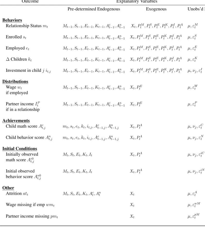
equations. Table 3.1 summarizes the jointly estimated set of 14 equations and their determinants.
The first column of Table 3.1 lists all the dependent variables of the system of equations, and
columns 2-4 contain the explanatory variables for each equation, including the pre-determined
en-dogenous variables, exogenous variables and unobserved heterogeneity. The probabilities formed
Table 3.1: Specification Summary for Jointly Estimated Set of Equations
Outcome Explanatory Variables
Pre-determined Endogenous Exogenous Unobs’d Het
Behaviors
Relationship Statusmt Mt−1, St−1, Et−1, Kt−1, Act−1, Atn−1 Xt, PtM, PtS, PtE, PtK, PtI, PtA µ, εMt
Enrolledst Mt−1, St−1, Et−1, Kt−1, Act−1, Atn−1 Xt, PtM, PtS, PtE, PtK, PtI, PtA µ, εSt
Employedet Mt−1, St−1, Et−1, Kt−1, Act−1, Atn−1 Xt, PtM, PtS, PtE, PtK, PtI, PtA µ, εEt
∆Childrenkt Mt−1, St−1, Et−1, Kt−1, Act−1, Ant−1 Xt, PtM, PtS, PtE, PtK, PtI, PtA µ, εKt
Investment in childj it,j Mt−1, St−1, Et−1, Kt−1, Act−1, Ant−1 Xt, PtM, PtS, PtE, PtK, PtI, PtA µ,νj, εIt
Distributions
Wagewt Mt−1, St−1, Et−1, Kt−1, Act−1, Ant−1 Xt, PtE µ, εWt if employed
Partner incomeItP Mt−1, St−1, Et−1, Kt−1, Act−1, Ant−1 Xt, PtE µ, εPt if in a relationship
Achievements
Child math scoreAc
t,j mt, st, et, kt, it,j, Act−1,j, Atn−1,j Xt, PtA µ,νj, εCt
Child behavior scoreAn
t,j mt, st, et, kt, it,j, Act−1,j, Atn−1,j Xt, PtA µ,νj, εNt
Initial Conditions
Initially observed Mt, St, Et, Kt, It Xt, PtA µ,νj, εiCt
math scoreAc0
t,j
Initial observed Mt, St, Et, Kt, It Xt, PtA µ,νj, εiNt
behavior scoreAn0
t,j
Other
Attritionatt Mt, St, Et, Kt, Act, Ant Xt µ, εAt
Wage missing if empwmt Xt µ, εwMt
3.4 Likelihood Function
The unconditional likelihood function for womanzis given by:
Q X q=1 θq ( T Y t=1 X2 m=0
p(mzt =m|Ωzt, µq)1(mzt =m)
X1
s=0
p(szt=s|Ωzt, µq)1(szt =s)
× 5 X
e=0
p(ezt =e|Ωzt, µq)1(ezt=e)
X1
k=−1
p(kzt =k|Ωzt, µq)1(kzt =k)
× 1 X
a=0
p(atzt=a|Ωzt, µq)1(atzt=a)
X1
b=0
p(wmzt =b|Ωzt, µq)1(wmzt =b)
× 1 X
c=0
p(pmzt =c|Ωzt, µq)1(pmzt =c)
×φW(wzt|Ωzt, µq)1(ezt≤3)1(wmzt=0)φP(IztP|Ωzt, µq)1(mzt6=2)1(pmzt=0)
× J Y j=1 R X r=1 δr
φAc0(Acztj0 |Ωzt, µq, νr)φA
n0
(Anztj0|Ωzt, µq, νr)
1(j≤Kzt+kzt)
×
T
Y
t=1
φI(iztj|Ωzt, µq, νr)φAc(Acztj|Ωzt, µq, νr)φAn(Anztj|Ωzt, µq, νr)
1(j≤Kzt+kzt))
(3.10)
where a womanz faces type q permanent heterogeneity, µq, with probability θq, and her child j
faces typer permanent heterogeneity, νr, with probabilityδr. pX(·) is the probability for
behav-ior/outcomeX, ifX is a discrete variable; φX(·)is the probability density for behavior/outcome
X, if X is a continuous variable. They are derived from the equations listed in Table 3.1. The
parameters of the likelihood function are estimated with full information maximum likelihood.
3.5 Identification
Identification of the causal effects of family structure on children’s achievements requires that
there are exogenous variables that are correlated with the joint behaviors, but do not have
inde-pendent impacts on children’s achievements other than through behavioral inputs. This exclusion
restriction requirement is satisfied by the timing assumption of the model, and the time-varying
state and local variables that represent the price and supply side conditions, such as local marriage
First, within each periodt, women living in different states/counties may experience different
combinations of state and local environments. All of these state and local variables of periodt,Pt,
enter into the behavior equations (3.1)-(3.5), as they may jointly influence women’s behaviors. But
conditional on the period t observed behaviors, only state and local factors that may affect
chil-dren’s achievements, namely those representing local school characteristics, enter into the child
achievement production equations. For example, local unemployment rates in periodtmay affect
a woman’s schooling and labor supply, but conditional on women’s schooling status, employment
status, and accumulated human capital stock in periodt, these unemployment rates do not affect
their children’s achievements independently. Therefore, they are excluded from children’s
achieve-ment production functions, and serve as within-period exclusion restrictions.
Second, the identification also comes from across-period exclusion restrictions. Namely, even
women living in the same community in periodt, may have different location histories, therefore
may have experienced varying state and local environments before periodt. All these state and
local environments before periodthave influenced women’s past endogenous behaviors, which in
turn affect their behaviors in periodt. Again, conditioning on women’s behaviors in periodt, these
past state and local environment variables do not have independent effects on children’s
achieve-ments in periodt, therefore serving as additional exclusion restrictions. For example, the variation
in state-level average college tuitions in periodt−1could affect women’s schooling status in
pe-riodt−1, which then may influence women’s schooling status in periodt- an input for children’s
achievement production functions in period t. Conditional on the women’s enrollment status in
periodt, the variations of state-level average tuitions in t−1 do not have an independent effect
on children’s achievements in periodt. Therefore, they implicitly serve as across-period exclusion
restrictions for children’s achievement production functions in period t. In fact, all the state and
local environment variables before periodt, serve such purpose. The exclusion restrictions used in
CHAPTER 4
DATA
I use panel data from the National Longitudinal Survey of Youth 1979 (NLSY79) and the
NLSY79 Children and Young Adults (NLSY79-CS). The NLSY79 is a nationally representative
sample of 12,686 young men and women who were 14 to 22 years old when they were first
sur-veyed in 1979. These individuals were interviewed annually through 1994 and are currently
inter-viewed on a biennial basis. In addition to demographic information such as gender, race, ethnicity,
and date of birth, the survey also provides detailed information on their relationship, employment,
and fertility at each wave. Starting from 1986, the NLSY79 began to interview all children born
to female NLSY79 respondents. For each child, the survey gathers information on measures of
children’s cognitive and non-cognitive achievements, as well as parental investment in each child.
My research sample includes women who have not attrited by 1986 and who were observed for
at least two consecutive periods (1986 and 1987). I exclude the military subsample, whose
deci-sion making process is likely to be different from the rest of the NLSY79 sample. I also excluded
the economically disadvantaged, nonblack/non-Hispanic subsample, which was discontinued from
1990. I follow 4,395 women and 8,579 children from 1986 to 2012 or until the first time they
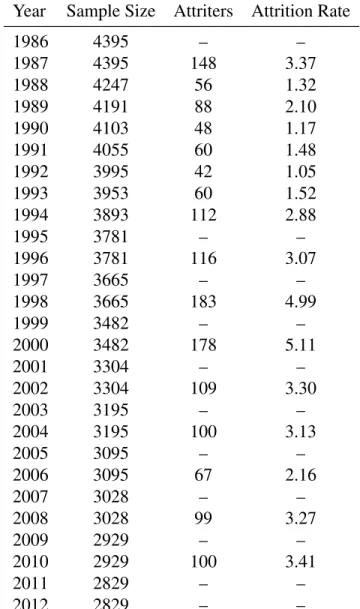
attrit-ted from the NLSY79 survey. Table 4.1 shows the research sample size and attrition of adults by
year. The research sample contains 95,843 adult-year observations, and the attrition rate by wave is
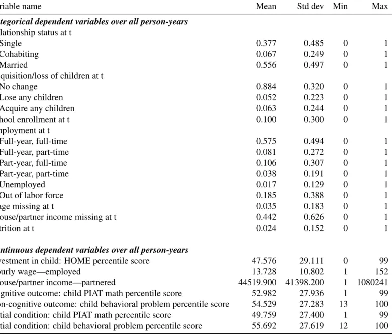
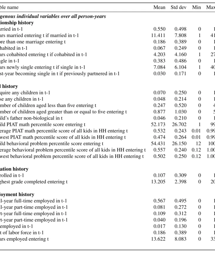
generally below 5 percent. Tables 4.2 - 4.5 display descriptive statistics for the dependent variables,
endogenous explanatory variables, exogenous explanatory variables, and state/local environment
Table 4.1: Empirical Distribution of Research Sample
Year Sample Size Attriters Attrition Rate
1986 4395 – –
1987 4395 148 3.37
1988 4247 56 1.32
1989 4191 88 2.10
1990 4103 48 1.17
1991 4055 60 1.48
1992 3995 42 1.05
1993 3953 60 1.52
1994 3893 112 2.88
1995 3781 – –
1996 3781 116 3.07
1997 3665 – –
1998 3665 183 4.99
1999 3482 – –
2000 3482 178 5.11
2001 3304 – –
2002 3304 109 3.30
2003 3195 – –
2004 3195 100 3.13
2005 3095 – –
2006 3095 67 2.16
2007 3028 – –
2008 3028 99 3.27
2009 2929 – –
2010 2929 100 3.41
2011 2829 – –
2012 2829 – –
Table 4.2: Descriptive Statistics for Dependent Variables
Variable name Mean Std dev Min Max
Categorical dependent variables over all person-years
Relationship status at t
Single 0.377 0.485 0 1
Cohabiting 0.067 0.249 0 1
Married 0.556 0.497 0 1
Acquisition/loss of children at t
No change 0.884 0.320 0 1
Lose any children 0.052 0.223 0 1
Acquire any children 0.063 0.244 0 1
School enrollment at t 0.100 0.300 0 1
Employment at t
Full-year, full-time 0.575 0.494 0 1
Full-year, part-time 0.081 0.272 0 1
Part-year, full-time 0.106 0.307 0 1
Part-year, part-time 0.038 0.191 0 1
Unemployed 0.017 0.129 0 1
Out of labor force 0.185 0.388 0 1
Wage missing at t 0.035 0.183 0 1
Spouse/partner income missing at t 0.442 0.626 0 1
Attrition at t 0.024 0.152 0 1
Continuous dependent variables over all person-years
Investment in child: HOME percentile score 47.576 29.111 0 99
Hourly wage—employed 13.728 10.802 1 152
Spouse/partner income—partnered 44519.900 41398.200 1 1080241
Cognitive outcome: child PIAT math percentile score 52.982 27.936 1 99
Non-cognitive outcome: child behavioral problem percentile score 54.529 27.283 13 100
Initial condition: child PIAT math percentile score 49.759 27.400 1 99
Initial condition: child behavioral problem percentile score 55.692 27.619 12 100
Table 4.3: Descriptive Statistics for Endogenous Individual Explanatory Variables
Variable name Mean Std dev Min Max
Endogenous individual variables over all person-years
Relationship history
Married in t-1 0.550 0.498 0 1
Years married entering t if married in t-1 11.411 7.808 1 41
More than one marriage entering t 0.186 0.389 0 1
Cohabited in t-1 0.067 0.249 0 1
Years cohabited entering t if cohabited in t-1 4.203 4.160 1 27
Single in t-1 0.383 0.486 0 1
Years newly single entering t if single in t-1 7.084 6.104 1 40
First-year becoming single in t if previously partnered in t-1 0.030 0.171 0 1
Child history
Acquire any children in t-1 0.070 0.250 0 1
Lose any children in t-1 0.048 0.214 0 1
Number of children aged less than five entering t 0.247 0.520 0 4
Number of children aged greater than or equal to five entering t 0.877 1.030 0 5
Child’s father non-biological in t 0.046 0.210 0 1
Child PIAT math percentile score entering t 52.173 26.702 1 99
Average PIAT math percentile score of all kids in HH entering t 0.532 0.243 0.01 0.99 Lowest PIAT math percentile score of all kids in HH entering t 0.474 0.264 0.01 0.99
Child behavioral problem percentile score entering t 54.431 26.150 12 100
Average behavioral problem percentile score of all kids in HH entering t 0.557 0.240 0.12 1.00 Lowest behavioral problem percentile score of all kids in HH entering t 0.502 0.250 0.12 1.00
Education history
Enrolled in t-1 0.107 0.309 0 1
Highest grade completed entering t 13.205 2.398 0 20
Employment history
Full-year full-time employed in t-1 0.567 0.495 0 1
Full-year part-time employed in t-1 0.081 0.272 0 1
Part-year full-time employed in t-1 0.109 0.312 0 1
Part-year part-time employed in t-1 0.040 0.196 0 1
Unemployed in t-1 0.017 0.130 0 1
Out of labor force in t-1 0.186 0.389 0 1
Table 4.4: Descriptive Statistics for Exogenous Individual Explanatory Variables
Variable name Mean Std dev Min Max
Time-invariant individual variables in year 1986
Black race 0.305 0.460 0 1
Hispanic 0.185 0.388 0 1
AFQT score 41.003 28.260 0 100
AFQT score missing 0.031 0.174 0 1
Country of birth: non-U.S. 0.066 0.247 0 1
Residence at age 14: non-U.S. 0.022 0.146 0 1
Residence at age 14 missing 0.002 0.045 0 1
Birthplace of mother: non-U.S. 0.103 0.304 0 1
Birthplace of mother missing 0.003 0.050 0 1
Birthplace of father: non-U.S. 0.097 0.296 0 1
Birthplace of father missing 0.024 0.153 0 1
Highest grade completed of mother 10.798 3.191 0 20
Mother’s education missing 0.053 0.223 0 1
Highest grade completed of father 10.926 3.912 0 20
Father’s education missing 0.147 0.354 0 1
Time-variant individual variables over all person-years
Age in years 36.869 8.076 21 56
Child age 6.223 4.063 1 17
Female child 0.487 0.500 0 1
Rural residence 0.230 0.421 0 1
Residence type missing 0.024 0.153 0 1
Northeast region 0.158 0.365 0 1
North central region 0.235 0.424 0 1
South region 0.419 0.493 0 1
West region 0.188 0.391 0 1
Region missing 0.006 0.078 0 1
State of residence missing 0.010 0.099 0 1
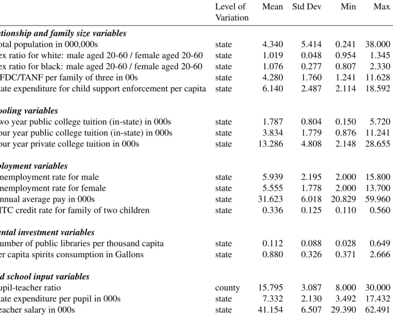
Table 4.5: Descriptive Statistics for Exogenous Price and Supply-Side Variables
Level of Mean Std Dev Min Max
Variation
Relationship and family size variables
Total population in 000,000s state 4.340 5.414 0.241 38.000
Sex ratio for white: male aged 20-60 / female aged 20-60 state 1.019 0.048 0.954 1.345 Sex ratio for black: male aged 20-60 / female aged 20-60 state 1.076 0.277 0.807 2.330
AFDC/TANF per family of three in 00s state 4.280 1.760 1.241 11.628
State expenditure for child support enforcement per capita state 6.140 2.487 2.114 18.592
Schooling variables
Two year public college tuition (in-state) in 000s state 1.787 0.804 0.150 5.720
Four year public college tuition (in-state) in 000s state 3.834 1.779 0.876 11.241
Four year private college tuition in 000s state 13.286 4.808 2.148 28.655
Employment variables
Unemployment rate for male state 5.939 2.195 2.000 15.800
Unemployment rate for female state 5.555 1.778 2.000 13.700
Annual average pay in 000s state 31.623 6.018 20.829 59.960
EITC credit rate for family of two children state 0.336 0.125 0.110 0.560
Parental investment variables
Number of public libraries per thousand capita state 0.112 0.088 0.028 0.649
Per capita spirits consumption in Gallons state 0.880 0.326 0.371 2.666
Child school input variables
Pupil-teacher ratio county 15.795 3.087 8.000 30.000
State expenditure per pupil in 000s state 7.332 2.130 3.492 17.432
Teacher salary in 000s state 41.154 6.507 29.390 62.491
4.1 Description of Key Variables
A goal of this dissertation is to understand the effects of family structure on child achievements.
Figure 4.1 depicts the probabilities of each family structure (single, cohabiting, married) over the
life cycle for the cohort of women in my sample. The probability of women being married increases
sharply in their twenties’ from 28% to 55%, while the their probability of being single plummets
from 63% to 36%. Both probabilities become more stable starting from age 30. The probability of
cohabitation, on the other hand, decreases slowly and steadily throughout their life cycle, with an
average of 6.7%.
Family structure is closely related to other maternal behaviors that may also influence children’s
cognitive and non-cognitive development. Maternal human capital, including education and work
experience, could affect children’s development through channels such as parenting practices or
the role model effect. As Panels A and B in Figure 4.2 show, the distribution of the schooling
and employment status differ by family structure types, with single women most likely to enroll in
school and work full-year and full-time. Another factor that could impact the resource availability
for the child is the family size. Panel C in Figure 4.2 shows that women who are married are
more likely to have a child in their 20’s and 30’s, compared with cohabiting or single women.
The probability is reversed after women reach their 40’s. Lastly, parental investment is associated
with family structure. Panel D of Figure 4.2 shows that married mothers invest the most in their
children and single mothers invest the least (in terms of average investment). To the extent that
all these behaviors interact with family structure types, and could potentially impact children’s
achievements, it is important to account for the endogeneity of such behaviors over the life cycle
in order to identify the unbiased causal impacts of family structure.
For the measure of parental investment, the NLSY79-CS assesses the home environment of
children using the Home Observation Measurement of the Environment-Short Form (HOME-SF).
HOME-SF includes four sets of questions that depend on the age of the child: ages 0–2, 3–5, 6–9
and 10 and above. One part of the HOME-SF is self-administered by the mother of the child,
Figure 4.1: Family Structure Probabilities at Age t
how many times, if any, have you had to spank child in the past week (to mothers of children
aged 3-5). The other part is the interviewer’s observation, with questions such as whether mother
encouraged child to contribute to the conversation (observed by the interviewer).1 These questions
are designed to measure the cognitive stimulation and emotional support from the mother, and I
use the age-specific HOME-SF percentile scores as the measure of investment in children.
To measure child cognitive achievement, I use the Peabody Individual Achievement Test (PIAT)
math score provided in the NLSY79-CS. PIAT is among the most widely used brief assessment of
academic achievement for children aged five or over. The majority of children in the NLSY79-CS
have more than three valid PIAT scores, making it possible to estimate women’s time-varying
in-vestment in children and the evolution of their children’s cognitive achievements. The PIAT math
test measures a child’s attainment in mathematics. It consists of 84 multiple-choice items of
in-creasing difficulty, ranging from early skills as recognizing numerals and progresses to measuring
advanced concepts in geometry and trigonometry. The PIAT math percentile scores I use are
de-rived on an age-specific basis from children’s PIAT math raw scores. Panel A of Figure 4.3 shows
that both boys and girls from married households have significantly higher math scores, compared
to their peers in single or cohabiting households.
To measure child non-cognitive achievement, I use the Behavior Problem Index (BPI), created
by Peterson and Zill (1986) and collected by the NLSY79-CS to measure the frequency, range, and
type of childhood behavior problems for children age four and over. The BPI used in the
NLSY79-CS includes 28 questions administered to mothers of each child, asking about specific behaviors
in the following domains: (1) antisocial behavior, (2) anxiousness/depression, (3) headstrongness,
(4) hyperactivity, (5) immature dependency, and (6) peer conflict/social withdrawal. The BPI
per-centile scores I use are derived on age-specific BPI raw scores, the higher of which indicate more
severe behavior problems. Panel B of Figure 4.3 shows that behavior problems are significantly
Figure 4.3: Children’s Achievements by Family Structure
4.2 Exogenous Prices and Supply-side Variables
I obtain the state/county-level aggregate variables that capture exogenous price and policy
vari-ations from the following data sources: (1) the school quality data, measured by pupil-teacher ratio,
teacher salary and expenditure per child, comes from the Common Core Data (CCD); (2) the
col-lege tuition data, serving as price variation for school enrollment, comes from the National Center
for Education Statistics; (3) the local employment statistics and average wages come from the
Bu-reau of Labor Statistics; (4) the data on EITC policies comes from the Tax Policy Center; (5) the
data on welfare policies from 1986 to 1995 comes from Fang and Keane (2004) and Bernal and
Keane (2011), and the data from 1996 to 2012 comes from the Welfare Rules Database collected by
the Urban Institute; (6) the data on the number of public libraries comes from Institute of Library
and Museum Service, and (7) the data on alcohol consumption comes from National Institutes of
CHAPTER 5
ESTIMATION RESULTS
5.1 Replication of Previous Literature
Before estimating the preferred model specified in the previous chapter, I estimate the
reduced-form models commonly used in the literature using my research sample of women and their
chil-dren. The purpose of this section is two-fold: 1) it demonstrates that I find similar results regarding
the effects of family structure on children’s outcomes when using the common approaches, and 2)
it reinforces the differences in estimated marginal impacts when one accounts for selection and
endogeneity bias manifested in unobservable permanent characteristics of the household or the
child.
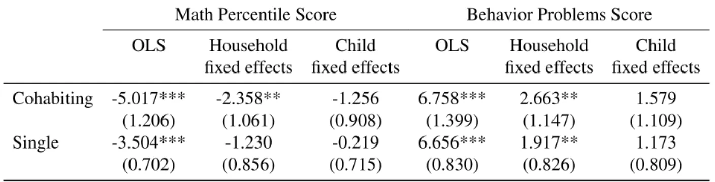
Table 5.1 presents the coefficients for alternative specifications of children’s cognitive and
non-cognitive production functions, including OLS, household fixed effects, and child fixed effects,
us-ing my research sample. For children’s cognitive production function, the OLS regression shows
that comparing with living in a married household, living in a cohabiting household statistically
significantly decreases children’s PIAT math scores by 5.02 percentage points, while living with a
single mother decreases children’s math scores by 3.50 percentage points. When using the
house-hold fixed effects model, which eliminates the unobserved heterogeity shared across siblings within
the same household, the magnitude of the effect of cohabitation reduces to 2.36 percentage points,
and the effect of living in single households becomes statistically insignificant. When using the
child fixed effects model, which eliminates the child-specific permanent unobserved heterogeneity,
the effects of both cohabitation and singleness become statistically insignificant.
For the production function of children’s non-cognitive achievement, Table 5.1 shows
household increases children’s behavioral problems by 6.76 and 6.66 percentage points,
respec-tively, the magnitudes of these effects are smaller after accounting for household-level unobserved
heterogeneity, and become statistically insignificant after eliminating child-specific permanent
un-observables. The changes of coefficients in these alternative specifications emphasize the existence
of the household-level and child-specific unobserved heterogeneity, which could potentially bias
the estimates if not properly accounted for. In the dynamic multiple equation model below, I
explicitly model both levels of unobserved heterogeneity and estimate their distributions.
These results are consistent with findings from the literature examining the effects of family
structure on children’s outcomes. Using household or child fixed effects to account for unobserved
heterogeneity, the literature generally finds that the negative impacts of unmarried parenthood on
children’s outcomes become smaller or statistically insignificant, compared to results from OLS
regressions. For example, using data from both the NLSY79 and the Panel Study of Income
Dynamics (PSID), Bj¨orklund et al. (2007) show that the negative impacts of non-intact family
types (including single mother, single father, stepmother, stepfather families) on children’s
edu-cational attainment become statistically insignificant with household fixed effects. Aughinbaugh
et al. (2005) also find that the negative effects of divorce on children’s PIAT Math score and
Be-havioral Problem Index score disappear after using child fixed effects.1
1Aughinbaugh et al. (2005) use the raw scores of PIAT Math and Behavioral Problem Index for children in the
Table 5.1: Alternative Specifications of Achievement Production Functions
Math Percentile Score Behavior Problems Score
OLS Household Child OLS Household Child
fixed effects fixed effects fixed effects fixed effects
Cohabiting -5.017*** -2.358** -1.256 6.758*** 2.663** 1.579
(1.206) (1.061) (0.908) (1.399) (1.147) (1.109)
Single -3.504*** -1.230 -0.219 6.656*** 1.917** 1.173
(0.702) (0.856) (0.715) (0.830) (0.826) (0.809)
Note: Robust standard errors in parentheses. *** p<0.01, ** p<0.05, * p<0.1. Explanatory vari-ables include an indicator for non-biological father, the age, race and gender of the child, women’s age, education level, and region of residence, time trend, and indicators for missing values.
5.2 Results from the Dynamic Dynamic Multiple-equation Model
This section discusses the key findings using the estimated dynamic multiple-equation model.
I first test how the estimated model fits the observed data. Then, I use the estimated coefficients
to discuss factors that influence women’s family structure and patterns displayed in children’s
achievement production functions. Lastly, I calculate the contemporaneous and life-cycle marginal
effects of family structure on children’s cognitive and non-cognitive achievements.
5.2.1 Model Fit
It is important that the estimated model captures the patterns displayed in the observed data.
I use the estimated parameters to simulate women’s life-cycle behaviors and their children’s
out-comes from the first period forward, and use the simulated values of endogenous explanatory
variables to update behaviors and outcomes in the next period. The comparison of the summary
statistics for the simulated behaviors and outcomes with the observed data in Table 5.2 suggests
that the estimated model fits the data well.
5.2.2 Estimated Coefficients
Results from estimation of the correlated set of equations are detailed in Appendix Tables
A.5-A.19. The coefficients on endogenous explanatory variables are listed first followed by those for
exogenous variables and unobserved heterogeneity. Here I focus my discussion on the key
Table 5.2: Summary Statistics for Model Fit
Outcomes Observed Simulated
Mean Std. Dev. Mean Std. Dev.
Relationship Status
Married 0.556 0.497 0.551 0.497
Cohabiting 0.067 0.249 0.069 0.254
Single 0.377 0.485 0.379 0.485
School Enrollment 0.100 0.300 0.110 0.313
Employment Status
Full-year full-time employed 0.575 0.494 0.561 0.496
Full-year part-time employed 0.081 0.272 0.084 0.278
Part-year full-time employed 0.106 0.307 0.104 0.305
Part-year part-time employed 0.038 0.191 0.039 0.195
Unemployed 0.017 0.129 0.018 0.132
Out of labor force 0.185 0.388 0.193 0.395
Family Size Changes
Have a chid 0.063 0.244 0.061 0.240
Lose a child 0.052 0.223 0.038 0.191
No change 0.884 0.320 0.901 0.299
Parental investment
HOME percentile score 0.476 0.291 0.475 0.260
Child Achievements
PIAT Math percentile score 0.523 0.278 0.515 0.285
BPI behaviral problem percentile score 0.547 0.273 0.540 0.285
Wage and Income
Hourly wage 13.73 10.80 13.62 8.30
Spouse/Partner income 44518.86 41398.52 44680.61 43114.62
Note: Hourly wage and spouse/partner income are in year 2000 dollars.
and their standard errors are shown in Appendix Table A.5 and A.6, in which the reference
re-lationship status is married, and the alternative statuses are cohabiting and single, respectively.
The coefficients on relationship history display three features. First, there exist self-sustaining
ef-fects within each relationship status. That is, being in a relationship status last period increases
the probability of choosing the same relationship status in the current period. In addition, as the
duration of a particular relationship status increases, it is more likely that the woman stays in the
same relationship. Second, singleness and cohabitation reinforce each other. That is, being single
period. Similarly, cohabiting last period increases the chance of being single over married this
period. The third finding is that the same past life-cycle behavior may have varying roles when it
comes to choosing alternative relationship status (cohabiting/single) versus marriage. For example,
after having a child in the last period, a woman is less likely to choose singleness over marriage,
but she is no less likely to choose cohabitation over marriage. Another example is that
unemploy-ment increases the woman’s probability of being single over married, but it does not impact the
probability between cohabitation and marriage. One endogenous factor that has consistent impacts
on relationship choice is the woman’s education level. More educated women are more likely to
choose marriage both over cohabitation and over singleness.
The estimated coefficients of the correlated set of equations also provide empirical support
for the existence of complementarity of parental investments, and the self-productivity of skills.
Appendix Table A.15 shows that parents invest more in children who have lower behavioral
prob-lems, which is consistent with the theory of static complementarity of parental investment (Cunha
et al., 2006). In addition, Appendix Tables A.18 and A.19 display that non-cognitive achievement
promotes the formation of cognitive achievement, but cognitive achievement in general do not
pro-mote the formation of non-cognitive achievement. The same patterns of the self-productivity of
skills are found in Cunha and Heckman (2008).
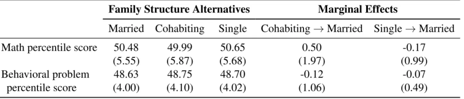
5.2.3 Estimates of the Contemporaneous and Life-cycle Marginal Effects
In order to understand the dynamic impacts of family structure on children’s achievements,
I first calculate the effects of a one-period change in family structure from cohabiting or single
household to married household on children’s contemporaneous achievements. That is, holding
everything else the same, if the child is living in a married rather than a cohabiting or single
house-hold this year, how might her cognitive and non-cognitive development differ in the same year? I
call this thecontemporaneous (or one-period) effect. Table 5.3 shows that the contemporaneous
effects are statistically insignificant, indicating that children’s cognitive and non-cognitive
achieve-ments are not immediately affected by changes in family structure.
A lack of contemporaneous effects does not necessarily imply that family structure does not