DATA ACQUISITION, ANALYSIS, AND MODELING OF ROTORDYNAMIC SYSTEMS
A Thesis
presented to
the Faculty of California Polytechnic State University,
San Luis Obispo
In Partial Fulfillment
of the Requirements for the Degree
Master of Science in Mechanical Engineering
by
Michael Mullen
COMMITTEE MEMBERSHIP
TITLE: Data Acquisition, Analysis, and Modeling of Rotordynamic Systems
AUTHOR: Michael Mullen
DATE SUBMITTED: June 2020
COMMITTEE CHAIR: Dr. Xi Wu, Ph.D.
Professor of Mechanical Engineering
COMMITTEE MEMBER: Dr. Eltahry Elghandour, Ph.D. Professor of Mechanical Engineering
ABSTRACT
Data Acquisition, Analysis, and Modeling of Rotordynamic Systems
Michael Mullen
ACKNOWLEDGMENTS
Thanks to:
• David Baker, Cameron Naugle, and Gregg Pelligrino
• Dr. Xi Wu, Dr Eltahry Elghandour, and Dr. Hemanth Porumamilla
• George D’Entremont
• Aaron Hampton, Bently Nevada
TABLE OF CONTENTS
Page
LIST OF TABLES . . . x
LIST OF FIGURES . . . xi
CHAPTER 1 Introduction . . . 1
1.1 Importance of Vibration Analysis . . . 1
1.2 Literature Review . . . 4
1.3 Scope . . . 6
1.4 Vibration Measurements Overview . . . 7
1.4.1 Amplitude . . . 8
1.4.2 Frequency . . . 10
1.4.3 Phase . . . 11
1.4.4 Time Domain vs Frequency Domain . . . 11
2 Equipment Overview . . . 13
2.1 Proximity Probes . . . 13
2.2 Bently Nevada Data Acquisition Systems . . . 19
3 Modeling . . . 20
3.1 Keyphaser Simulation . . . 20
3.1.1 Simulation for Constant Rotor Speed (ω=Constant) . . . 21
3.1.2 Simulation for Constant Angular Acceleration (α =Constant) 23 3.1.3 Laser Tachometer Simulation . . . 27
3.2 Transient System Response Simulation Method . . . 28
3.2.2 Model Rotor Ramp Simulation . . . 31
3.2.3 Anisotropic Rotor Ramp Simulation . . . 33
4 Data Processing Methods . . . 36
4.1 Data Processing Parameters . . . 36
4.1.1 Frequency Span (Fmax) Selection and Relation to Sampling Fre-quency (fs) . . . 37
4.1.2 Selection of Frequency Resolution (F F T Lines) . . . 41
4.1.3 Selection of a Full Scale Range . . . 49
4.2 Data Acquisition Methods . . . 50
4.2.1 Current Methods . . . 50
4.2.2 Batch Processing and Triggers . . . 51
4.2.3 Vector and Waveform Data . . . 51
4.2.4 State Based Acquisition . . . 52
4.3 Fourier Transforms and the Creation of Spectrum Plots . . . 53
4.3.1 Half Spectrum . . . 54
4.3.2 Full Spectrum . . . 61
4.3.3 Averaging . . . 68
4.4 Amplitude Calculations . . . 69
4.4.1 Max-Min Calculation . . . 69
4.4.2 RMS Conversion . . . 71
4.4.3 Derived Peak from FFT Spectra . . . 72
4.5 Phase Calculations . . . 73
4.5.1 Time Domain . . . 74
4.5.2 Frequency Domain . . . 78
4.6.1 Window Overlap . . . 87
4.6.2 Synchronous vs Asynchronous . . . 87
5 App Development . . . 91
5.1 Layout Design . . . 91
5.2 Feedback Loops . . . 95
5.3 Triggers . . . 96
6 Vibration Lab Upgrades . . . 98
6.1 Current Lab Setup . . . 98
6.2 Bently Nevada System 1 Evo Software . . . 99
6.3 Bently Nevada 2300/20 Vibration Monitors . . . 100
6.3.1 2300/20 Configuration . . . 101
6.3.2 Device Implementation . . . 104
6.4 Bently Nevada 3701 . . . 107
6.4.1 Configuration and Implementation . . . 108
6.4.2 System 1 Integration . . . 111
7 Conclusion . . . 116
7.1 Summary of Results . . . 116
7.2 Future Work . . . 117
7.2.1 ADAPT 3701/44 . . . 117
7.2.2 Potential Uses for Bently Nevada 2300/20 and System 1 . . . 117
7.2.3 Matlab App Development and Rolling Element Bearing Analysis118 BIBLIOGRAPHY . . . 120
APPENDICES A List of Variables . . . 123
C Bently Nevada ADAPT 3701/44 DataSheet . . . 143 D Bently Nevada ADAPT 3701/44 Setup Guide for Cal Poly Vibrations
LIST OF TABLES
Table Page
3.1 Simulation Input Parameters for X(t) Signal Generation . . . 32
3.2 Simulation Input Parameters for Anisotropic Rotor Simulation . . . 34
4.1 Allowable Frequency Spans (Fmax) and Lines of Resolution (F F T Lines) 44 4.2 Correction Factors and Error for Common Window Types . . . 48
4.3 Amplitude Measurement Methods Comparison . . . 73
4.4 Phase Measurement Methods Comparison . . . 82
LIST OF FIGURES
Figure Page
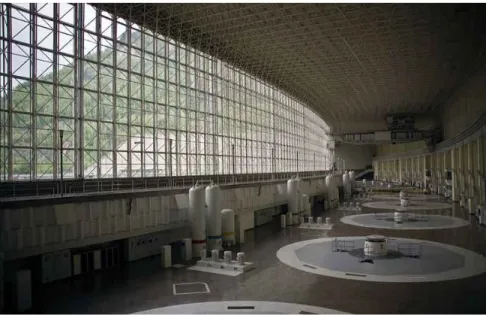
1.1 The generator deck of the Sayano-Sushenskaya hydroelectric power
plant as seen on June 25th, 2009. [11] . . . 2
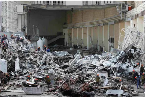
1.2 The generator deck of the Sayano-Sushenskaya hydroelectric power plant following the accident. [11] . . . 3
1.3 Bently Nevada RK4 RotorKit . . . 7
1.4 Steady State Vibration Signal of a Sine Wave With a Frequency of 25 hz and Peak to Peak Amplitude of 2 . . . 8
1.5 Time domain and Frequency Domain of Equation Created in section 4.3.1 (1000 hz span and 800 lines) . . . 12
2.1 X-Y Proximity Probes on a Bently Nevada Rotorkit . . . 13
2.2 Bently Nevada Proximitor Assembly for RK4 Rotor Kit . . . 14
2.3 Aluminum Wheel for Torsional Vibration Measurement . . . 16
2.4 Radial Shaft Size Sensitivity for 3300 Probes [14] . . . 17
2.5 Axially Offset Vertical and Horizontal Proximity Probes on RK4 Rotor Kit . . . 18
3.1 Simulated Keyphaser Signal Generated in Matlab . . . 20
3.2 Diagram of a Shaft Cutaway Used to Approximate the Keyphaser Signal . . . 22
3.3 Matlab Code for Keyphaser Pulse Simulation . . . 23
3.4 Matlab Code for Loading Keyphaser Pulse Time array for Constant Acceleration . . . 25
3.5 Simulated Transient Keyphaser Signal . . . 26
3.7 Simulation of a Laser Tachometer Keyphaser signal using Matlab Rectpuls Function . . . 28 3.8 Rotor Ramp Simulation using Table 3.1 Parameters X(t) Signal Bode
Plot . . . 32 3.9 Rotor Ramp Simulation X(t) using Table 3.1 Parameters Time
Wave-form with Bode Plot Overlays . . . 33 3.10 Bode Plot of Realistic Ramp Simulation for Anisotropic Rotor using
Table 3.2 Parameters . . . 34 3.11 Orbit Plots for Simulated Counter-Clockwise Rotation Anisotropic
Rotor Ramp using Table 3.2 Parameters . . . 35
4.1 Simulated Analog Signal of a Sine Wave with an Amplitude of 5 and Frequency of 50Hz . . . 38 4.2 Under Sampled Signal at n=1.5 Sampling Rate . . . 38 4.3 Reconstructed Signal From Discrete Samples at n=1.5 Sampling Rate 39 4.4 Signal Sampled at the Nyquist Threshold Rate N=2 . . . 39 4.5 Reconstructed Signal From Discrete Samples at N=2 Sampling Rate 40 4.6 Signal Sampled above Nyquist Threshold Rate N=2.56 . . . 40 4.7 Reconstructed Signal From Discrete Samples at N=2.56 Sampling
Rate . . . 41 4.8 Simplified Half Spectrum Plot Showing Relationship Between
Spec-tral Lines (F F T Lines) and Bin Width . . . 42 4.9 Fourier Transform of an Aperiodic Signal Resulting in Spectral Leakage 45 4.10 Aperiodic Time Domain Input Signal with Hanning Window
Appli-cation . . . 46 4.11 Hanning Window . . . 47 4.12 Converting Analog Sine Wave to Digital Signal with a 3 Bit A/D
4.15 Matlab Code for the Calculation of the Half Spectrum . . . 56
4.16 Double Sided Spectrum of 2048 point FFT . . . 57
4.17 Double Sided Spectrum After Applying fftshift() Function . . . 57
4.18 Matlab Code for Calculating the Frequency Array of FFT . . . 58
4.19 Symmetric Full Spectrum Plot of Single Signal Input . . . 59
4.20 Matlab Code for Calculating the Frequency Bins of the Half Spectrum 60 4.21 Half Spectrum Plot of Equation 4.9 . . . 61
4.22 Matlab Code for Generating Complex Signal for Full Spectrum FFT 63 4.23 Matlab Code for Calculating Complex FFT for Full Spectrum Plots 63 4.24 Unshifted Double Sided Spectra of Complex Input Signal . . . 64
4.25 Double Sided Spectra of Complex Input Signal After Using fftshift() Function . . . 64
4.26 Double Sided Spectra of Complex Input Signal with Frequency Range to Nyquist Frequency . . . 65
4.27 Matlab Code for Trimming Full Spectrum Frequency Array for -fspan to +fspan . . . 65
4.28 Full Spectrum Example of Equations 4.10 and 4.11 where Ax = 2, Ay = 2, φx = 30◦, φy = 0, Fspan = 2000 hz, 400 Lines of Res-olution . . . 66
4.29 Forward Procession Example for Full Spectrum Plot of Equations 4.10 and 4.11 where Ax = 2, Ay = 2, φx = 0, φy = 0, Fspan = 2000 hz, 400 Lines of Resolution . . . 67
4.30 Reverse Procession Example for Full Spectrum Plot of Equations 4.10 and 4.11 where Ax = 2, Ay = 2, φx = 110◦, φy = 0, Fspan = 2000 hz, 400 Lines of Resolution . . . 67
4.31 Simulated Vibration Signal With Introduced Voltage Spike . . . 69
4.32 Matlab Code For Time Domain Amplitude Min-Max Calculation . 70 4.33 RMS Calculation of Vectors in Matlab . . . 71
4.35 Simulated X and Y signal with Keyphaser for Testing Phase
Mea-surement Methods . . . 74
4.36 Matlab Code for Locating Peaks in Time Waveform for Use in Phase Calculations . . . 75
4.37 Matlab Code for Calculating Absolute and Relative Phase from a Time Waveform Signal . . . 77
4.38 Matlab Code for Cutting Time Waveform at Keyphaser and per-forming FFT for Phase Analysis . . . 80
4.39 Matlab Code for Calculation of Phase in Frequency Domain . . . . 81
4.40 Time Waveform of Simulated Rotor Transient and Sample Time Waveform for FFT Processing,Fmax = 1000hz and F F T Lines = 800 83 4.41 Half Spectrum Plot of Transient Data with Short Time Span,Fmax = 1000hz and F F T Lines= 800 . . . 84
4.42 Half Spectrum Plot of Transient Data with Long Time Span,Fmax = 1000hz and F F T Lines= 6400 . . . 85
4.43 Cascade Plot of Data From Section 3.2.3 Using Batch Processing Method With Data Collection Every 2 Seconds and Frequency Span of 1000 hz and 400 Lines . . . 86
5.1 Matlab APP User Interface as Designed by David Baker [2] . . . . 92
5.2 Bently Nevada TK21 Oscilloscope Interface [13] . . . 93
5.3 Matlab DAQ App Front Page . . . 94
5.4 Matlab DAQ App Channel Configuration Page . . . 95
5.5 Matlab DAQ App Triggering Configuration Page . . . 96
6.1 Bently-Nevada 2300 Series Vibration Monitor [B] . . . 100
6.2 Bently-Nevada 2300/20 Monitor Local Configuration . . . 101
6.6 Bently-Nevada 2300/20 Enclosure and Mount . . . 106
6.7 Bently Nevada ADAPT 3701/44 Vibration Monitor . . . 107
6.8 Single ADAPT 3701/44 Common For Two RK-4 Rotor Kits . . . . 108
6.9 Bently Nevada ADAPT 3701/44 MAC Address Location . . . 109
6.10 Bently Nevada ADAPT 3701/44 Terminal Block Wiring Setup . . . 110
6.11 Bently Nevada RK-4 Proximeter Assembly Wiring for ADAPT 3701 111 6.12 System 1 Evo Machine Model for Rotor Kit 1 . . . 112
6.13 System 1 Bode Plot Data from Rotor Kit 1 Ramp . . . 113
6.14 System 1 Polar Plot from Rotor Kit 1 Ramp . . . 114
Chapter 1
INTRODUCTION
1.1 Importance of Vibration Analysis
The measurement of vibrations are vital in determining the current or future condition of all rotating machinery; however, the sophistication of those measurements are dependant on value of the rotating machinery both in physical cost, lost opportunity cost, and potential to cause harm in the event of failure.
The simplest of all vibration measurements are auditory. By merely listening to a machine and judging the pitch and magnitude of the sound, a technician can make inferences as to the condition of the machinery and in the case of a fault, can help diagnose the cause of root cause of vibration. For example, if an automobile is making an unusual noise that typically indicates a fault, which has caused an excessive vibra-tion that manifests itself as sound. The pitch, severity, duravibra-tion and circumstances surrounding the noise can help a technician diagnose the cause. A worn serpentine belt causes a higher pitch noise than a worn tensioner pulley. Although there are some tools such as a mechanics stethoscope or ChassisEAR which help aide in isolat-ing the source of the noise, the overall vibration measurement and interpretation of measurement in the automotive repair industry is quite rudimentary. Evaluation is subjective and generally based on technician experience.
the pecuniary value and potential harm to people or the environment is higher in this type of equipment, the level of sophistication of machinery condition monitoring must increase.
Figure 1.1: The generator deck of the Sayano-Sushenskaya hydroelectric power plant as seen on June 25th, 2009. [11]
The Sayano-Sushenskaya Hydroelectric power station is a 10 turbine, 6,500 MW Dam located in south-central Siberia. On October 3rd, 2009 the bolts holding down Turbine
Figure 1.2: The generator deck of the Sayano-Sushenskaya hydroelectric power plant following the accident. [11]
75 people were killed in the accident, 40 million tons of oil was released into the river below the dam and the cost to repair just the engine room alone would be an estimated 1.3 billion dollars not including economic impacts caused by the ensuing grid blackout [11].
1.2 Literature Review
Several textbooks were used in the creation of this thesis. Bently’s Fundamentals of Rotating Machinery Diagnostics [4], provides a good overview to data acquisi-tion, modeling, and applications to machinery diagnostics. Vance’s Rotordynamics of Turbomachinery [22], provides more in-depth information regarding instabilities in rotordynamics and computational methods for rotordynamic analysis; a short sec-tion also covers the measurement and analysis of torsional vibrasec-tions. Eisenmann’s Machinery Malfunction Diagnosis and Correction [19], is an excellent resource for practical implementation of vibration and rotordynamic theory for use in machinery diagnostics and predictive maintenance strategy. Muszynska’s Rotordynamics [15], provides thorough and detailed mathematical derivations for the modeling of various rotordynamic systems. Child’s Turbomachinery Rotordynamics [6], gives an excellent historical overview of the development of vibration analysis and rotordynamics over the past century, as well as many case studies on the applications of rotordynamic analysis in machinery diagnostics.
With regards to signal analysis, Fundamentals of Signal Processing for Sound and Vibration Engineers by Hammon and Shin [21] provides an overview on signal pro-cessing theory with many applications and examples shown in Matlab which can be downloaded from the Mathworks Website.
Cerna and Harvey’s white paper of the fundamentals of fft based signal Analysis and Measurement [5] gives an in-detail overview to the calculation of a half spectrum from sampled data, basic information on anti-aliasing and the application of windows.
generating half spectrum fft and the derivation of the Discrete Fourier Transform to Fast Fourier Transform.
GUo,Yu,Sun,Zhang and Zheng’s article on continuous and real time vibration data acquisition and analysis [10] provides an example of data acquisition with the empha-sis on hardware configuration and networking for vibration data acquisition rather than analysis.
Rossi, Valerio and Naldi, Lorenzo and Depau’s Torsional Vibrations in Rotordynamics Systems [20], covers newly developed non-intrusive methods of measuring torsional vibrations in-situ for the application of machinery protection.
Doan’s Apparatus for the Measuring of Torsional Vibrations [7], provides the elec-tronic methods used to measure torsional vibrations based of variation in pulse spacing using a proximity probe and toothed wheel.
Wachel, JC and Szenasi, Fred R and others [23] gives an in-depth example of a full torsional analysis of a rotor system including modeling, computational analysis and stress analysis.
Goldman and Muszy´nskas Application of Full Spectrum to Rotating Machinery Diag-nostics [9] provides an overview of the full spectrum plot, calculations for converting between full spectrum and orbit, and a list of common machinery conditions diag-nosed from the full spectrum plot.
Baxter’s Practical Applications of Signal Processing [3], provides a good explana-tion of the methods required in vibraexplana-tion data processing with an emphasis on the importance of batch processing and trouble shooting for machine ramp conditions.
Elbhbah, Keri and Sinha, Jyoti K [8], cover the use of a machine composite spectrum to enhance machinery condition monitoring with a limited number of measurement points.
1.3 Scope
kits. The Adapt 3701 with System 1 Evo was configured and proved to be capable to meet the requirements as a full replacement for the aging ADRE 208 systems.
1.4 Vibration Measurements Overview
This thesis will focus on measurements of relative shaft displacement using a proximity probe. The relative measurement refers to the displacement of the shaft relative to the bearing or machine. Normally this method of measurement would only be used on machinery with fluid film bearings since the amplitude of shaft displacement relative to the bearing gives a direct indication of the clearances within the bearing. All measurement were made on a the Bentley RK-4 Rotorkit shown in figure 1.3. The rotor kit utilizes bronze bushing but with a narrow flexible shaft. This enables relative motion between the rotor and the bearing supports despite having rigid bushings.
While displacement was the main form of measurement during this thesis, the meth-ods and techniques used to acquire and process data can be applied to data acquisition through accelerometers and velocimeters as well. Applications of the proximity probe and hardware setup considerations are covered in detail in section 2.1.
1.4.1 Amplitude
0 0.05 0.1 0.15 0.2 0.25 0.3 0.35 0.4 0.45 0.5
Time (s)
-1 -0.8 -0.6 -0.4 -0.2 0 0.2 0.4 0.6 0.8 1
Amplitude
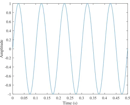
Figure 1.4: Steady State Vibration Signal of a Sine Wave With a Frequency of 25 hz and Peak to Peak Amplitude of 2
Figure 1.4 shows a simple sine wave with constant amplitude. Although this sine wave would be read as a changing voltage, the values can be converted into physical meaning by use of a manufacturer provided calibration constant. This sine wave represents an ideal signal which in reality is rarely as clean due to noise, nonlinearities in the system and the presence of other frequencies. The ideal signal could be described by the equation
Where X is the peak amplitude, ω is the frequency in rad/s, however in speaking hertz (hz) or cycles per second is a more commonly used unit
The magnitude of the vibration can be the acceleration, velocity, or displacement be-ing measured. Which measurement is used depends on accessibility to the source of vibration and the frequency range which is being measured. Proximity Probes mea-sure relative displacement and are adequate for low frequencies and typically used in measuring vibrations on machinery with fluid film bearings. Velocity transducers typically measure case vibrations since they have a wide frequency band of approxi-mately 10 hz to 1000 hz and velocity has a direct correlation to the kinetic energy of vibration. Therefore, it is the best indicator of the machinery damage. Accelerome-ters are used for a wide range of applications due to their ruggedness, wide frequency band and ability to capture high frequencies. A commonly used transducer for peri-odic vibration monitoring is the single integrating accelerometer. This provides many of the advantages of both; allowing for the capturing of high frequency data to help with diagnosing early stage bearing degradation and providing velocity values for comparison against vibration thresholds for machinery operation. A more in depth explanation of choosing measurement instrumentation can be found in other sources such as Vance[22] or Eisenmann [19].
Displacement
mil peak to peak (p-p). Alternatively, a root mean square measurement is often used since this value corresponds to the equivalent energy of vibration. In this case, a root mean squared (rms) value is often used. The rms value of a sine wave can be calculated from the peak or peak to peak value as seen below.
Vrms=Vp×0.707
Vrms=Vp−p×0.353
(1.2)
Since the amplitude is a constant for a steady state response, measuring the peak to peak amplitude is simple. We can measure the peak to peak amplitude using
Amplitudep−p =M ax(X(t))−M in(X(t)) (1.3)
Then the values for peak amplitude or rms can be calculated using the equation 1.2. X(t) is continuous as described in equation 1.1, however this method will also work for a properly sampled set of discrete values, as would happen during real data acquisition where voltages are recorded at certain time intervals. Amplitude measurement methods are described in section 4.4. These measurement conventions do not take any DC offset into account which is typically desired when looking at the dynamic motion. However, the DC offset or Gap Voltage is quite important to ensure the proximity sensor is within its effective range and to ensure that the rotor does not come into contact with the sensor.
1.4.2 Frequency
rpm is the standard unit. The period of vibration is the seconds required for one cycle to occur. This is the inverse of f and is an important measurement in the determination of sampling time since sufficient time must occur to sample a number of cycles at a low frequency.
1.4.3 Phase
Phase is the measurement of the offset between two signals. In this thesis both relative and absolute phase will be discussed. Relative phase is the phase angle between two dynamic signals of the same frequency. The absolute phase is the phase angle difference between a dynamic signal and a fixed once per revolution marker known as the Keyphaser. The phase is typically measured in units of radians but colloquially units of degrees are used. Phase measurement methods are described in section 4.5.
1.4.4 Time Domain vs Frequency Domain
0 0.2 0.4 0.6 0.8 Time (sec)
-2 -1 0 1 2
Amplitude
0 200 400 600 800 1000
Frequency (hz) 0
0.5 1 1.5 2 2.5
Amplitude
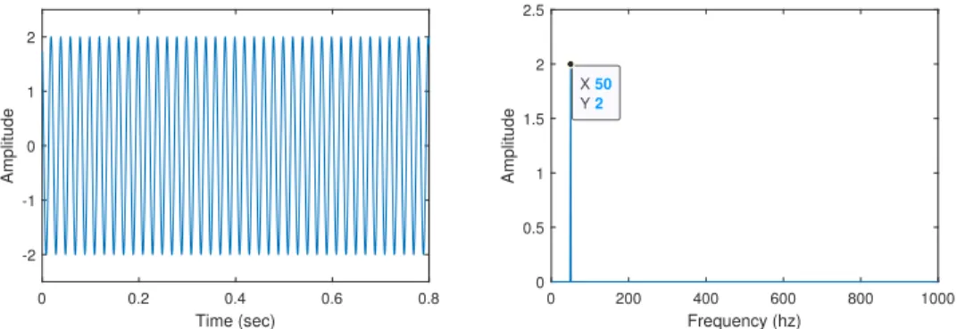
X 50
Y 2
Figure 1.5: Time domain and Frequency Domain of Equation Created in section 4.3.1 (1000 hz span and 800 lines)
Chapter 2
EQUIPMENT OVERVIEW
2.1 Proximity Probes
Figure 2.1: X-Y Proximity Probes on a Bently Nevada Rotorkit
Proximitor assemblies. In the case of the RK4 Rotor Kit Proximitor assembly the -24vdc supply comes from the motor controller instead.
Figure 2.2: Bently Nevada Proximitor Assembly for RK4 Rotor Kit
The Proximiter assembly has a high frequency oscillator internal which sends a small high frequency current through the inductor in the tip of the proximity probe. This high frequency circuit creates eddy currents on the surface of metallic objects nearby. The closer the metallic object, the more power the eddy currents consume. This is demodulated and then output as a signal voltage. So if the proximity probe is not near any metallic objects very little power is absorbed and the output voltage will be similar to the input voltage of -24vdc. However if the probe is in direct contact with a metal object then almost all of the power will be absorbed in the eddy currents and the output voltage will be near 0 vdc.
purposes of the lab they are equivalent with the exception of a different color wire (NSV has a blue wire as opposed to grey). The important specifications are identical and both are typical of common proximity probes. The proximity probes have a sensitivity of 200 mv/mil, a -24 vDC bias, a linear range of 60 mils, and a frequency response of 0 to 10kHz.
Figure 2.3: Aluminum Wheel for Torsional Vibration Measurement
the full scale range set in the data acquisition system may allow larger amplitudes to be displayed than those that are in the linear range of the transducer. More information on setting the full scale range is discussed in section 4.1.3. When using proximity probes for dynamic radial measurement on a shaft, size of the shaft can affect sensitivity. Figure 2.4 shows the approximate effect of shaft size on Average Scale Factor (sensitivity).
Figure 2.4: Radial Shaft Size Sensitivity for 3300 Probes [14]
also effect the measurement of a proximity probe. This effect is call cross-talk and is due to the interference from the eddie currents generated by each probe. This issue is often related to shaft size since the smaller the shaft the closer two x-y proximity probes will be. With a sufficiently large shaft, the cross-talk interference is negligible. To compensate for smaller shaft size an axial offset between the x and y probe can be used as seen in figure 2.5.
Figure 2.5: Axially Offset Vertical and Horizontal Proximity Probes on RK4 Rotor Kit
2.2 Bently Nevada Data Acquisition Systems
Chapter 3
MODELING
This chapter includes methods for generating simulated signals for the purpose of developing data acquisition systems. While previous researchers had developed a program for generating a simulated signal from solving the equations of motion, a more realistic model was created for keyphaser generation and a less computationally demanding model was created for the dynamic input signals modeling the proximity probe outputs. The use of the two programs developed in this thesis will allow for the more rapid development and troubleshooting of data acquisition systems for collecting rotordynamic vibrations.
3.1 Keyphaser Simulation
0 0.1 0.2 0.3 0.4 0.5 0.6 0.7 0.8 0.9 1
time (s) -0.7
-0.6 -0.5 -0.4 -0.3 -0.2 -0.1 0 0.1 0.2
voltage(v)
In the previous models used by Baker and Naugle, the Keyphaser signal was simulated by a sine wave with a frequency equivalent to the rotor speed. Then the positive peak of the sign wave would be used as the reference value for a Keyphaser spike. To simulate a transient or changing frequency, an array of different frequencies would be put in the sine wave array over the duration of the simulation. This led to errors in the actual frequency measured during the simulation because the frequency was dependant on the step size of the time array for the simulation. This method of simulating the Keyphaser was close but would cause phase issues if the simulation was running for longer lengths of time. A better Keyphaser simulation was developed to more accurately model the shape of the voltage signal produced by the Keyphaser pulse and to correctly simulate the change in frequency of pulses during ramp up or ramp down simulations. This keyphaser indication represents an AC coupled signal but a DC offset could be added easily if desired in the simulation.
3.1.1 Simulation for Constant Rotor Speed (ω=Constant)
Figure 3.2: Diagram of a Shaft Cutaway Used to Approximate the Keyphaser Signal
The length of this pulse width can be approximated by accounting for the angular velocity of the shaft ω in rad/s, the diameter of the shaft D, and the approximate angleγ that subtends the width of the sloth. This method assumes the slot width is small compared to the over diameter of the shaft. The angle γ can be approximated by assuming the width of the notch in the shaft is approximately the length of the arc that would complete a circular cross section of the shaft. The angle γ in radians can be found using equation 3.1 where Dand hhave the same units, typically inches or millimeters.
γ = h (D 2)
(3.1) The pulse width of a keyphaser pulse can then be approximated as the the time required for the shaft to rotate through the angleγ. This time in seconds is calculated using equation 3.2.
P W = γ
ω (3.2)
The time array is sampled at a rate of f s (samples/sec). The shaft is rotating at a frequency of W hz with units of hertz (cycle/sec).
1 %Generate the keyphaser pulse signal
2 %generate a negative skew left triangular signal with pulsewidth
3 %(amplitude of the pulse can be changed by multiplying by scalar)
4 key shape=-tripuls(t,pw,-1);
5 %Calculate time at which pulses occur
6 d=0:1/W hz:t end;
7 %Create pulse train for signal with duration of t, at time d
8 keyphaser=pulstran(t,d,key shape,fs);
Figure 3.3: Matlab Code for Keyphaser Pulse Simulation
To generated the Keyphaser signal the shape, magnitude and duration of each indi-vidual pulse is defined using the tripuls function. Thepw represents the pulsewidth (seconds) and the -1 function input defines the triangle as skew left. Then an array of times for when each pulse occurs is created. For a constant speed shaft, the spacing between each array entry is the period of rotation or the inverse of the frequency in hertz, Whz. Finally the pulstran function repeats the individual pulse signal at the
times calculated for each pulse to occur as defined in the array, d.
3.1.2 Simulation for Constant Angular Acceleration (α=Constant)
speed, creating an array of times at which each pulse occurs is simple as in figure 3.3. However, if the shaft is ramping up or down then both the spacing between each pulse and the width of the pulse itself is changing with time. To calculate these values the ramp rate, starting speed, and either duration time or end speed are required as inputs. The angle subtended by the keyphaser notch, γ, is a physical constant and remains the same as calculated in equation 3.1. For this simulation a constant ramp rate, α in units of rads2 was specified until the prescribed running speed had been
reached.
tf =
ωf −ω0
α (3.3)
Equation 3.3 uses three user defined inputs to calculate the final time of the ramp. ωf and ω0 represent the starting rotor speed and final rotor speed both with units
of rads . From total time of the simulation, the number of cycles must be calculated to determine the size of the array which will hold the time of each Keyphaser event. The total angular displacement of the rotor in radians can be determined through equation 3.4.
θtotal =
α 2tf
2
+ω0tf +φ0 (3.4)
The starting point of the simulation is arbitrary and controlled by φ0. For this
simulation it is assumed that φ0 = 0 so the simulation starts with a Keyphaser fire.
By dividing the total angular displacement by 2π the total number of cycles can be found.
Ctotal =
θtotal
2π (3.5)
Since array dimensions must be an integer the f loor() Matlab function is used to round down to the nearest whole cycle. Now an array of zeros can be created that is the length of the number cycles. The time at which each cycle occurs can be solved using equation 3.6 for thenth cycle and then loaded intonthslot in the array of zeros.
0 = α 2t
2+ω
The Matlab script below in figure 3.4 solves equation 3.6 for the time for each cycle using the roots function then stores the positive time value at which that keyphaser event occurs in the d array.
1 for n=1:floor(cycle total)
2 cycles=[(W ramp rad/2),W rad start,-2*pi*(n)];
3 r=roots(cycles);
4 d(n)=r(r≥0);
5 end
Figure 3.4: Matlab Code for Loading Keyphaser Pulse Time array for Constant Acceleration
Now that the time at which each pulse occurs has been calculated, the pulse width of each of those Keyphaser signals can be determined.To simulate the changing pulse width with a constant acceleration α equation 3.7 can be used.
P W = γ αt+ω0
(3.7)
Where α is the angular acceleration or ramp rate in rad
s and ω0 is the slow roll speed
0 0.5 1 1.5 2 2.5 3 3.5 4 4.5
time (s)
-0.7 -0.6 -0.5 -0.4 -0.3 -0.2 -0.1 0 0.1 0.2
voltage(v)
Figure 3.5: Simulated Transient Keyphaser Signal
It is worth noting that the sampling rate f s must be large enough to sample the keyphaser signal dip so its magnitude is below the hysteresis threshold. When simu-lating a transient the sample rate must apply at the smallest pulse width (i.e. max-imum rotating speed). A rule of thumb found by this researcher is described in equation 3.8.
f s > 5
M IN(P W) (3.8)
3.1.3 Laser Tachometer Simulation
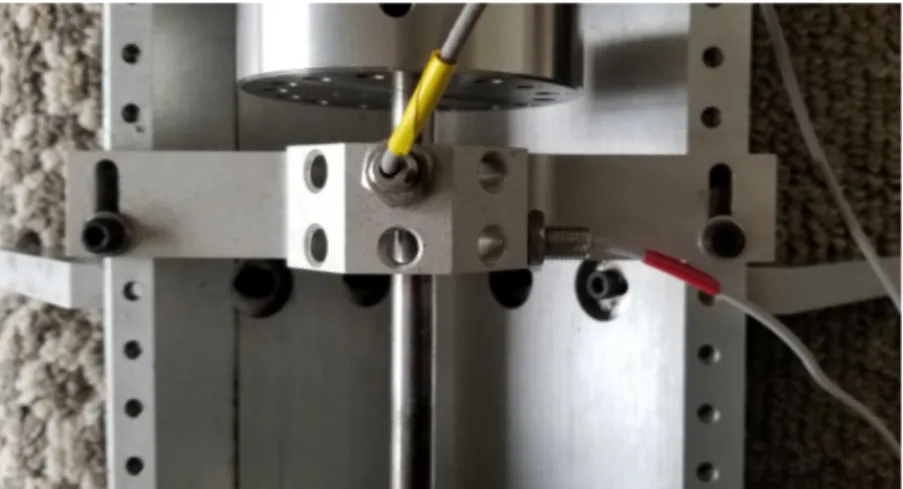
A commonly used instrument for generating a Keyphaser signal is a laser tachometer as seen in figure 3.6. A laser tachometer like the Monarch Pocket Laser Tach 200 uses a piece of reflective tape on a rotating surface to produce a once per revolution signal. The output of the laser tachometer is a 0 to 3.3Vdc TTL signal.
Figure 3.6: Monarch Laser Tachometer 200 used as Keyphaser Reference
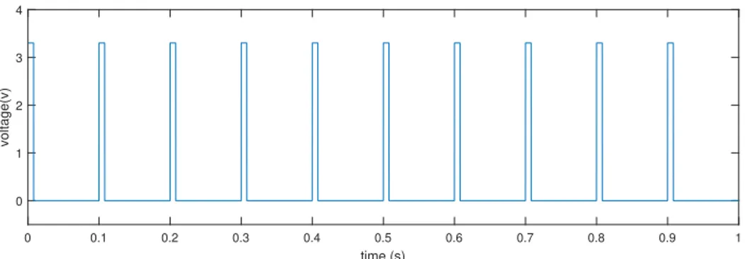
0 0.1 0.2 0.3 0.4 0.5 0.6 0.7 0.8 0.9 1 time (s)
0 1 2 3 4
voltage(v)
Figure 3.7: Simulation of a Laser Tachometer Keyphaser signal using Mat-lab Rectpuls Function
3.2 Transient System Response Simulation Method
3.2.1 Mathematical Modeling
This programs goal is provide quick simulations for use in the development and testing of a data acquisition system. Therefore the focus will be on simulating the kinematic response of a rotor system and ignoring the complexities in solving the kinetic equa-tions. The approach used provided a realistic model for data analysis prototyping although the methods used to create the signal are not mathematically derived. The fundamental building block of this simulation came from the Simple harmonic motion model in equation 3.9
X(t) =Asin(ωt+φ) (3.9)
For a steady state system this is can be a good representation of a transducer signal with primarily 1X vibration. If we base our model off a forced vibration single degree of freedom model then amplitude and phase can be described as a function ofr which is the ratio of the driving frequency to the natural frequency, ωn, of the system. In
the Jeffcott rotor model, which solves for the 1X vibration, the driving frequency ω is the rotating speed of the rotor.
r= ω ωn
(3.10) Then the amplitude, A can be described in equation 3.11.
A= p 1
(1−r2)2 + (2ζr)2 (3.11)
and the phase of the resulting vibration can be described in equation 3.12 φ= tan-1
2ζr 1−r2
(3.12) This simulation uses equation 3.13 to model the 1X vibration of a rotor undergoing acceleration at a constant ramp rate, α. The model is based of the simple harmonic motion model but includes a time varying amplitude, and phase as well as an accel-eration component in the angle component of the trig function.
X(t) = A(t)sin(α 2t
2+ω
Instead of determining the angle of the response for zero angular acceleration such as in 3.9 now a α
2t
2 term has been included to account for the acceleration component.
Previous researchers had used a model in which an ω array was created for each point in time of the simulation, then for each value of t in 3.9 the corresponding ω was inserted to calculate the position at that point in time. However this generated frequency errors where the final ”running speed frequency” for a ramp up simulation did not match what the simulation created. The incorporation of the acceleration term to determine the angle of the trig function resolved this issue.
To create a corresponding orthogonal signal, a cosine function was used to describe the Y signal as shown in 3.14.
Y(t) =A(t)cos(α 2t
2
+ω0t+φ(t)) (3.14)
Although in this case both the Y(t) andX(t) signal use the same time varying Am-plitude function,A(t) and phase function,φ(t), theY(t) andX(t) signals could have their own independent function Ax(t),Ay(t), φx(t), φy(t), to simulate an anisotropic
rotor condition. This can be done by selecting a newωn andζ in equations 3.16 and
3.18. For a constant ω, the frequency ratio r was constant as defined in equation 3.10. Since ω is now changing with time the constant r described in equation 3.10 cannot be used. This equation must be altered to solve for the rotational speed as a function. The standard kinematic formula in equation 3.15 can be used to solve for ω(t).
ω(t) =αt+ω0 (3.15)
Substituting ω(t) into r from equation 3.10 results in a time dependant r(t) shown in equation 3.16. This can be solved for each individual time step to create an r(t) vector which can then be used to solve equations 3.17 and 3.18
r(t) = αt+ω0 ωn
The functions for amplitude A(t) and phaseφ(t) were modeled after the steady state response of a forced vibration model which is commonly found in any vibrations textbook, equations 3.11 and 3.12. Using ther(t) solved in equation 3.16, arrays can be created for the amplitude A(t) and phaseφ(t).
A(t) = p A0
(1−r(t)2)2 + (2ζr(t))2 (3.17)
Where A0 represents the slow roll amplitude or amplitude at low frequencies relative
to the natural frequency.
φ(t) = tan-1
2ζr(t) 1−r(t)2
(3.18) Equations 3.17 and 3.18 now show a slight difference from the forced vibration model as the r, the ratio of driving frequency to natural frequency described in equation 3.10 is now a function of time, r(t). The the amplitudes A(t) and phases φ(t) can now be used to solve equations 3.13 and 3.14 to create an X and Y signal that varies amplitude, frequency and phase with time in accordance to the inputs of the system described below.
3.2.2 Model Rotor Ramp Simulation
The practical implementation of this method in Matlab would be to define the desired parameters of the simulation such as sampling frequency,fs, starting speed,ω0, ramp
rate, α, final speed, ωf, the desired natural frequency speed,ωn, and then a damping
ratio for the system, ζ. The selection of a zeta is often iterative to produce a result satisfactory to the user. Once these parameters have been defined the simulation time can be calculated using the following equation:
tf inal =
ωf −ωo
α (3.19)
Then a time vector can be created from 0 to tf inal in increments of f1s. This vector
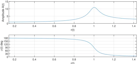
Then this vector can be used to solve equation 3.17 and 3.18 to create vectors for the amplitude and phase at each point in time. Finally the vectors for amplitude, A(t), and phase, φ(t) can be used to generate a simulated signal for the X and Y probes using equations 3.13 and 3.14. For an example the following inputs in table 3.1 were used to generate an X(t) signal. The speeds used are lower than typical to allow for the frequency change in the time waveform to be easily seen in figure 3.9.
Table 3.1: Simulation Input Parameters for X(t) Signal Generation
fs ω0 ωf α ωn ζ A0
2560 hz 50 rpm 500 rpm 1000 rpm/min 350 rpm 0.05 1
Using the Inputs from table 3.1, the final time(tf inal) of the simulation was calculated
using equation 3.19. Then a time array and ther(t) array was created using equation 3.16. This r(t) was used to calculate theA(t) and φ(t) arrays.
0.2 0.4 0.6 0.8 1 1.2 1.4
r(t) 0
5 10 15
Amplitude A(t)
0.2 0.4 0.6 0.8 1 1.2 1.4
r(t) 0
30 60 90 120 150 180
(t) deg
Figure 3.8: Rotor Ramp Simulation using Table 3.1 Parameters X(t) Signal Bode Plot
as a bode plot and also commonly shows the amplitude and phase as a function of running speed instead of frequency ratio.
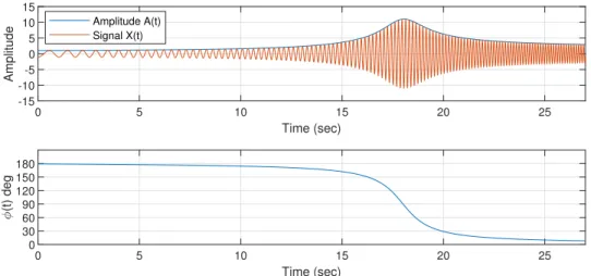
0 5 10 15 20 25
Time (sec) -15
-10 -5 0 5 10 15
Amplitude
Amplitude A(t) Signal X(t)
0 5 10 15 20 25
Time (sec) 0
30 60 90 120 150 180
(t) deg
Figure 3.9: Rotor Ramp Simulation X(t) using Table 3.1 Parameters Time Waveform with Bode Plot Overlays
After calculating the time dependant amplitude and phase the entire time waveform can now be generated using equation 3.13. In figure 3.9 the generated X(t) signal is shown with amplitude from the bode plot overlaid. This method of simulation has the advantage of being very quick to generate; the example in this section took less than 5 seconds of computation time. This is very quick compared to the several minutes required by previous methods which involve solving the ODE’s. This simulation model will be very useful in the testing of DAQ systems. By varying ramp rates and decreasing the damping ratio, ζ, the limitations of the acquisition methods can be quickly found.
3.2.3 Anisotropic Rotor Ramp Simulation
signal should be defined in equations 3.16 and 3.18. Then individual amplitudes Ax(t),Ay(t), and phasesφx(t), φy(t) can be input into the X and Y signals. Since the
signals represent the X and Y transducers of a rotor undergoing a ramp, the sampling frequency, fs, starting speed, ω0, ramp rate,α and final speed, ωf will all remain the
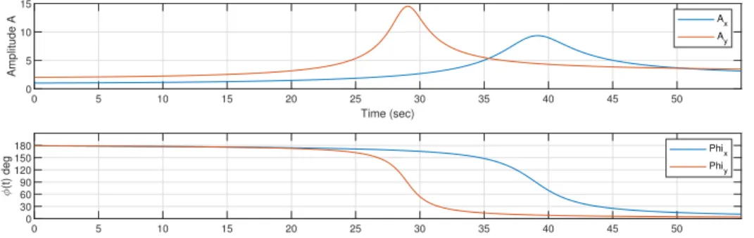
identical for the X and Y signals. For this example the following parameters in table 3.2 were used to simulate the ramping of an anisotropic rotor from 250 rpm to 300 rpm. This is consistent with ramping of the Bently Nevada RK-4 rotor kits. The natural frequencies (ωn) and damping ratios (ζ) of each signal were arbitrarily chosen
for this example.
Table 3.2: Simulation Input Parameters for Anisotropic Rotor Simulation
Signal fs ω0 ωf α ωn ζ A0
X(t) 2560 hz 250 rpm 3000 rpm 3000 rpm/min 2200 rpm 0.06 1 Y(t) 2560 hz 250 rpm 3000 rpm 3000 rpm/min 1700 rpm 0.04 2
0 5 10 15 20 25 30 35 40 45 50
Time (sec)
0 5 10 15
Amplitude A
Ax Ay
0 5 10 15 20 25 30 35 40 45 50
Time (sec)
0 30 60 90 120 150 180
(t) deg
Phix
Phiy
Figure 3.10: Bode Plot of Realistic Ramp Simulation for Anisotropic Rotor using Table 3.2 Parameters
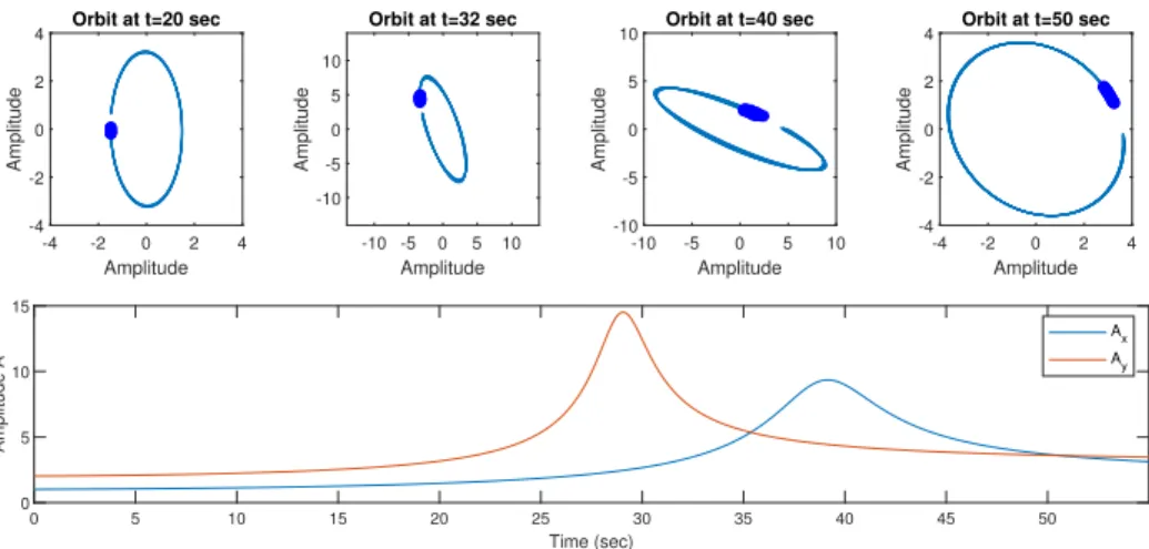
be easily changed to represent a more drastic imbalance in the rotor and evaluate the limits of the data acquisition method in use.
0 5 10 15 20 25 30 35 40 45 50
Time (sec) 0 5 10 15 Amplitude A Ax Ay
-4 -2 0 2 4
Amplitude -4 -2 0 2 4 Amplitude
Orbit at t=20 sec
-10 -5 0 5 10 Amplitude -10 -5 0 5 10 Amplitude
Orbit at t=32 sec
-10 -5 0 5 10
Amplitude -10 -5 0 5 10 Amplitude
Orbit at t=40 sec
-4 -2 0 2 4
Amplitude -4 -2 0 2 4 Amplitude
Orbit at t=50 sec
Figure 3.11: Orbit Plots for Simulated Counter-Clockwise Rotation Anisotropic Rotor Ramp using Table 3.2 Parameters
Chapter 4
DATA PROCESSING METHODS
This chapter covers data processing methods for rotordynamic systems. Before ac-quiring data, initial parameters must be defined to dictate how long to take data and at what rate to sample the data. Once data is collected, processing methods exist in both the frequency and time domain to acquire measurements used in analysis of the machine condition. Various methods for the calculation of amplitudes and phase angles from time domain and frequency domain were created for implementation in Matlab. The conversion from the time domain to the frequency domain through the use of the Fourier transform is covered extensively. Data acquisition methods to maximize computational efficiency and minimize memory use are discussed as well as methods applied to minimize error and maximize efficiency during the acquisition of transient data which occurs on start-up conditions.
4.1 Data Processing Parameters
4.1.1 Frequency Span (Fmax) Selection and Relation to Sampling Frequency
(fs)
One of the main parameters selected during the setup of a data acquisition system is the frequency span orFmax (which are used interchangeably), which is the maximum
frequency that can be represented. Typically this number is in hertz and normally several orders of magnitude larger than running speed; however this can vary based of the type of machinery that is being analyzed. For instance a 3 blade axial fan with rolling element bearings and a 6 pole motor would require a much lower Fmax than
a high speed gearbox. Typically not any value can be selected for a Fmax. Usually
there are options of discrete values such as 500, 1000, 2000, 4000, or 5,000 hz. The reason for these specific values is discussed in section 4.1.2. Table 4.1 provides a list of commonly used frequency spans (Fmax).
With most DAQ’s the sampling rate is indirectly selected through the choosing of a frequency span. That is the sampling rate is some multiple of Fmax, typically 2.56.
The reason for using these specific discrete values for Fmax is that when multiplied
by 2.56 the amount of data that is sampled is a power of two. This allows for a computationally efficient calculation of the Fourier transform. This topic is covered in detail in section 4.3.1. However the multiple of the sampling rate must be at least greater two because of the Nyquist Criterion. The Nyquist criterion shown in equation 4.1 states the minimum sampling rate to be able to accurately recreate an analog signal
For the purposes of the data acquisition system and as an example to showcase the importance of this ratio, the sampling rate has been defined in equation 4.2 where n is a rational number.
fs =nFmax (4.2)
The following examples will showcase the importance of the selection of this number and errors that occur with under sampling signals where the recreation of the signal is known as aliasing. To help prevent this low pass filters known as anti-aliasing filters can be used.
0 0.05 0.1 0.15 0.2 0.25 0.3 0.35 0.4 0.45 0.5
Time (s)
-5 0 5
Amplitude
Figure 4.1: Simulated Analog Signal of a Sine Wave with an Amplitude of 5 and Frequency of 50Hz
A simulated analog sine wave is created with an Amplitude of 5 at a frequency of 50 hz. This analog wave will now be sampled at several different rates for n.
0 0.05 0.1 0.15 0.2 0.25 0.3 0.35 0.4 0.45 0.5
Time (s)
-5 0 5
Amplitude
Analog Signal Sampled Signal (n=1.5)
The signal is sampled at a rate of 75 hz (n=1.5) where each red marker indicates a discrete value recorded. This frequency is below the Nyquist Criterion and will result in an error when reconstructing the signal.
0 0.05 0.1 0.15 0.2 0.25 0.3 0.35 0.4 0.45 0.5
Time (s) -5
0 5
Amplitude
Sampled Signal (n=1.5) Recreated Signal
Figure 4.3: Reconstructed Signal From Discrete Samples at n=1.5 Sam-pling Rate
In figure 4.3 the digital signal sampled in figure 4.2 is reconstructed using the curve fitting toolbox within MatLab. In all scenarios presented in this section a ”fourier8” fit was used within the Matlab curve fitting toolbox. The resulting reconstructed curve is significantly different than the original simulated analog signal and has a fundamental frequency much lower than the original.
0 0.05 0.1 0.15 0.2 0.25 0.3 0.35 0.4 0.45 0.5
Time (s)
-5 0 5
Amplitude
Analog Signal Sampled Signal (n=2)
In the scenario shown in figure 4.4 the simulated analog signal is sampled at a rate of 100 hz (n=2). The Nyquist Criterion must be greater than 2 so the Nyquist Criterion is not met in this scenario either
0 0.05 0.1 0.15 0.2 0.25 0.3 0.35 0.4 0.45 0.5
Time (s) -5
0 5
Amplitude
Sampled Signal (n=2) Recreated Signal
Figure 4.5: Reconstructed Signal From Discrete Samples at N=2 Sampling Rate
With a sampling rate at twice the frequency of the input signal that reconstructed signal shown in figure 4.5 is approximately zero and the original signal was not accu-rately reconstructed
0 0.05 0.1 0.15 0.2 0.25 0.3 0.35 0.4 0.45 0.5
Time (s)
-5 0 5
Amplitude
Analog Signal Sampled Signal (n=2.56)
Figure 4.6: Signal Sampled above Nyquist Threshold Rate N=2.56
0 0.05 0.1 0.15 0.2 0.25 0.3 0.35 0.4 0.45 0.5
Time (s)
-5 0 5
Amplitude
Sampled Signal (n=2.56) Recreated Signal
Figure 4.7: Reconstructed Signal From Discrete Samples at N=2.56 Sam-pling Rate
The reconstructed signal from the sampled data matches the simulated analog signal and shows that the sampling rate was sufficient to accurately analyze a signal of this frequency.
While in the development of a data acquisition system the 2.56 ratio is important, the end user of the software typically selects an Fmax only. However, it is important
to know the effects of Fmax selection and ensuring that theFmax is much higher than
any frequencies of interest for the machinery being analyzed. This emphasizes the importance of have sufficient understanding of the machine being analyzed as have an Fmax set too low could obscure energy in higher frequency bands that indicates
machinery faults or anomalies.
4.1.2 Selection of Frequency Resolution (F F T Lines)
less than 3600 rpm so the actual 2X running speed may be 116hz instead of 120hz. If too low of a frequency resolution is used then both of these signal would be lumped together in the same bins and it would be indistinguishable. This problem would increase the difficulty of determining a correct diagnosis.
Figure 4.8: Simplified Half Spectrum Plot Showing Relationship Between Spectral Lines (F F T Lines) and Bin Width
The frequency resolution of an FFT is typically referred to in terms of lines,F F T Lines. The lines represent the number of Fourier components calculated in the spectrum from the DC value, 0 hz, to the frequency span, Fmax. Select options for resolution are
typically 200, 400, 800, 1600, 3200, 6400 lines. Figure 4.8 shows an example of the fft lines of resolution. The shaded regions represent the bin for each line of resolution. The bin width can be calculated in equation 4.3
BW = Fmax
F F T Lines (4.3)
resolution. While higher resolution is generally preferred to enable the discretion of peaks with close frequencies, the drawback is that the increased resolution requires a longer time sample. The time required for the sample can be calculated in equation 4.16 which is the inverse of the bin width.
ts=
F F T Lines Fmax
(4.4)
The importance of only using select options for number of line (F F T Lines) and frequency span (Fmax) is to ensure the number of samples that get passed to the fft
function is a power of two. From the previous section we can calculate our sampling frequency (fs) as 2.56 times our frequency span as seen in equation 4.5.
fs = 2.56Fmax (4.5)
With the sampling time (ts) calculated in equation 4.16 the number of samples can
be calculated from equation 4.6 below.
Nsamples=tsfs (4.6)
By ensuring that the only options for the number of lines and the frequency span are those prescribed in table 4.1 the number of samples (Nsamples) will always be a power
Table 4.1: Allowable Frequency Spans (Fmax) and Lines of Resolution
(F F T Lines)
Frequency Span (Fmax) Lines of Resolution (F F T Lines)
10,000 12,800
5,000 6,400
4,000 3,200
2,000 1,600
1,000 800
500 400
400 200
Note: Any combination of Fmax and F F T Lines can be used.
Any combination of the values from table 4.1 will result in a sample length of a power of two. This ensures maximum computational efficiency when performing a Discrete Fourier Transform by using a Fast Fourier Transform (FFT) instead. An FFT can only be performed when the input signal contains a power of two number of samples. The calculation of the transforms is covered in section 4.3.
The frequency resolution is inversely proportional to sampling time span. Equation 4.7 shows the calculation for determining the frequency resolution,freswhich would be
the smallest resolvable difference between two frequencies of interest in the frequency spectra. The frequency resolution can be increased by either selecting a greater number of lines for a constant frequency span, Fmax, or by decreasing the frequency
span and holding the number of lines constant. Again both methods would result in increasing the time span for sampling.
fres=
2FmaxW F
However, equation 4.7 is not exactly the inverse of 4.16 since it incorporates a factor of two and a window factor, W F. The factor of 2 in 4.7 ensures there is at least one bin between two signals. If the two frequencies are in adjacent bins then they would appear as one wide peak as opposed to two individual peaks. The window factor, W F accounts for the increased leakage due to the application of window functions which are cover in section 4.1.2 below. Commonly used window factors are listed in table 4.2.
Window Functions
When sampling data, the signal often ends up being aperiodic, meaning if the signal was repeated end to end, each end would have a discontinuity. Performing a fourier transform on an aperiodic signal results in spectral leakage. Spectral leakage occurs where the energy contained within a signal leaks out into adjacent frequency bins.
0 0.05 0.1 0.15 0.2 0.25 0.3 0.35
Time (sec)
-5 0 5
Amplitude
Raw Input Signal
0 50 100 150 200 250 300 350 400 450 500
Frequency (Hz)
1 2 3 4 5
Amplitude [mils]
Half Spectrum of Signal Without Hanning Window Applied
Figure 4.9: Fourier Transform of an Aperiodic Signal Resulting in Spectral Leakage
this sample section. If this signal was perfectly periodic then the spectrum would result in a line only at 50 hz. However, in figure 4.9 the bins adjacent to the 50hz bin contain some amplitude as a result of not using a periodic signal. To force a signal to be periodic the input signal can be multiplied by another signal called a window, which is of the same number of points as the input signal but force each end of the input signal to zero, thereby making it always periodic. One of the most commonly used windows is called a hanning window. The hanning window is also commonly called a hann window. The hanning window is a special gaussian curve. By multiplying the input signal term by term with the hanning window, the ends of the signal are forced to zero.
0 0.05 0.1 0.15 0.2 0.25 0.3 0.35
Time (sec) -5
0 5
Amplitude
Raw Input Signal
0 0.05 0.1 0.15 0.2 0.25 0.3 0.35
Time (sec) 0
0.5 1
Amplitude
Hanning Window
0 0.05 0.1 0.15 0.2 0.25 0.3 0.35
Time (sec) -5
0 5
Amplitude
Input Signal with Hanning Window Applied
Figure 4.10: Aperiodic Time Domain Input Signal with Hanning Window Application
0 0.05 0.1 0.15 0.2 0.25 0.3 0.35
Time (sec)
-5 0 5
Amplitude
Input Signal With Hanning Window Applied
0 50 100 150 200 250 300 350 400 450 500
Frequency (Hz)
1 2 3 4
Amplitude
Half Spectrum of Signal Without Hanning Window Applied
Figure 4.11: Hanning Window
Table 4.2: Correction Factors and Error for Common Window Types
Window Type Amplitude Correction
Window Factor (W F)
Maximum Error
Uniform 1.0 1.0 37%
Hanning 2.0 1.5 15%
Flat Top 4.8 3.8 0.1%
4.1.3 Selection of a Full Scale Range
Selection of a full scale range is determine by the desired amplitude resolution of the signal and dependant upon the number of bits of the Analog to Digital (A/D) converter built in to the DAQ. The A/D converter takes a continuous analog electric signal and then converts into a series of steps where each step is represented by a binary number.
Figure 4.12: Converting Analog Sine Wave to Digital Signal with a 3 Bit A/D Converter
For example, in figure 4.12 a 3 bit A/D converter could have numbers ranging from 000 to 111, so the total number of discrete steps the signal could be broken into would be 23 = 8. The size of each of these steps determines the minimum resolvable
amplitude of an AC signal. If a full scale range of ±F S is used with a N-bit A/D converter then the minimum resolvable amplitude,Amin can be calculated in equation
4.8.
Amin =
2F S
2N (4.8)
For equation 4.8 the units of Amin and F S are the same, usually either mils or volts.
2.1.The default configuration used for the Bently Nevada 208 uses a full scale rang of 20mils. Any measured amplitude greater than 20 mils results in an error and gets clipped, a common issue during the single-plane balancing lab. The ADRE for Win-dows, software allows a full scale range of up to 50 mils. Since the ADRE 408, 2300, and ADAPT 3401 DAQs all use a 24 bit A/D converter, the worst amplitude resolu-tion would be 5×10⁻⁶ mils . This is well below the noise level due to electromagnetic
interference and surface defects read by the proximity probes. Therefore the maxi-mum full scale value of±50milsshould be used to avoid clipping high amplitudes of vibration so long as the linear range of the transducer is considered.
4.2 Data Acquisition Methods
Once the key parameters discussed in section 4.1 are chosen, the remaining variables necessary to collecting data can be calculated by the methods covered in this section.
4.2.1 Current Methods
4.2.2 Batch Processing and Triggers
As opposed to continuously collecting data over a long time period and then trying to cut it up in manageable pieces for data processing, a more efficient method is batch processing. Batch processing takes short collections of data and then processes that data. The length of each data collection depends on the inputs described in the previous section 4.1. So depending on the frequency resolution the time span for data collection could be long or short. How often data is collected depends on triggers, which are just a set of conditions. When the conditions are met a data collection begins. Common triggers are time or rotor speed. For instance triggers could be defined as every 5 seconds and a change of 25 rpm. The DAQ will begin taking data when the DAQ is started however it is only recording data into a buffer to evaluate the condition of the triggers. If 5 seconds hasn’t past or if a 25rpm change hasn’t occurred then the data in the buffer is deleted. If the conditions of the trigger have been met then a data collection will begin and the data will be saved and processed. This method has the advantage of reducing the total amount of data trying to be transmitted from the DAQ to the computer and can be configured to ignore certain states such as before the rotor begins to ramp. An example showcasing data taken with batch processing at a collection rate of every 2 seconds can be seen in the cascade plot in figure 4.43.
4.2.3 Vector and Waveform Data
phase. Examples of vector data would be overall amplitude, 1X amplitude and phase, 0.5x amplitude and phase, 2X amplitude and phase etc. This data can be stored more at a higher frequency because the entire spectral components of the window and the time waveform do not need to be saved. Vector data can be presented in plots such as bode, polar, trend, and shaft centerline plots. Waveform data consists of an entire time waveform collection and the spectral components calculated by the fft. The waveform data can be represented by half and full spectrum, cascade, waterfall, orbit, and time waveform plots. This data requires much more storage and typically is stored less frequently.
The application of this method allows the user to customize storage rates depending on the intended use of the data. For example in the ME318 lab student perform a single plane balance on a RK4 rotor kit. This requires the use of the 1X amplitude and phase in the form of a bode or polar plot. In this case only vector data is being used; therefore, the collection of waveform data could be eliminated entirely to optimize data storage use.
4.2.4 State Based Acquisition
speed values constitute the set points for each state. Then within each state, indi-vidual triggers can be defined as described in sections 4.2.2 and 4.2.3. For instance when operating at Slow Roll, the measurements such as amplitude and phase are rel-atively constant and contain no dynamic information so very few measurements are need. During transients the rotating speed is changing so the acquisition time of each collection must be shortened so the frequency stays relatively constant within each collection period. Once at running speed is reached the frequency remains constant and higher resolution data with longer sampling times can be used.
4.3 Fourier Transforms and the Creation of Spectrum Plots
The new method utilized is consistent with industry practices and is a much more efficient method of calculating the FFT. To create a spectrum, first the desired fre-quency span and lines of resolution must be selected. By only giving select values for frequency span and number of lines of resolution we can ensure that the number of samples recorded in the sampling time is a power of 2. Selection of a frequency span is covered in section 4.1.1, and selection of resolution is covered in section 4.1.2. A range of valid frequency spans and lines of resolution is listed above in table 4.1.
4.3.1 Half Spectrum
An example of the data processing used in Matlab will be shown for equation 4.9 which is a cosine function with a frequency of 50 hz (314.16 rad/s), amplitude of 2 and a phase of 30 degrees (π6 radians).
X(t) = 2cos(314.16t+π
6) (4.9)
1 %Calculate time array
2 %Calculate Sampling Rate
3 Fs=2.56*fspan; %samples/sec
4 %Calculate total sampling time
5 t s=lines/fspan; %sec
6 %Create time array with time step inverse of the sampling rate.
7 t=(0:1/Fs:t s -(1/Fs)); %sec
8 %Create the signal
9 x=A1*cos((w*t)+deg2rad(phix));
Figure 4.13: Matlab Code for Half Spectrum Generation of 4.9
The sampling rate is calculated as 2560 samples per second (2560 = 2.56×1000hz) and the total sampling time is calculated in line 5 of figure 4.13 using equation 4.16 (0.8seconds = 8001000lineshz ). A time array is created at the sampling rate and since the initial point is zero in the array the last step must be the sampling time minus one time step in order for the length of the time array to be a power of 2 (2048samples= 2560samplessec ×0.8seconds). The signal in line 9 of figure 4.13 creates the time waveform signal shown below in figure 4.14.
0 0.1 0.2 0.3 0.4 0.5 0.6 0.7 0.8
Time (sec) -2
-1 0 1 2
Amplitude
The sampled array, x, the sampling rate, Fs, and the frequency span, fspan, are passed to another function to calculate the FFT.
1 %Perform FFT and scale by number of points
2 Xfft=fft(X)/N;
3 %Take absolute value to find the magnitude of each component
4 X2 = abs(Xfft);
5 %Shift FFT spectrum to center to create single sided spectrum
6 X1 = 2*fftshift(X2);
Figure 4.15: Matlab Code for the Calculation of the Half Spectrum
The built in matlab function fft() performs the fast fourier transform on a set data and then is scaled by N, which is the length of the sampled data, in this case 2048. Previous researchers ensured the FFT of x was calculated to a power of 2 using the nextpow2() function in matlab. This finds the next highest power of two from the length of sample data. This value can then be put within the matlab fft() function and matlab will automatically pad the signal and calculate the fft to the next highest power of 2 points. By selecting certain frequency spans and lines of resolution this is no longer needed. The output of the fft function, Xfft, is an array 2048 points long made up of complex numbers. Each complex number represents a magnitude and angle for a corresponding bin.
centered about the halfway point of the number of points in the fft. For a single input signal the positive frequency components and the negative frequency components are complex conjugates so the full spectrum provides redundant information; however, the shortening of the full spectrum enables the creation of the half spectrum.
0 200 400 600 800 1000 1200 1400 1600 1800 2000
Spectral Points
0 0.5 1 1.5
Magnitude
X 41 Y 1
X 2009 Y 1
Figure 4.16: Double Sided Spectrum of 2048 point FFT
The spectrum above starts at the DC value or zero frequency value then all values until the mid point of the series are the positive frequency components. The midpoint is 1024 and represents the Nyquist frequency. All values after the Nyquist frequency correspond with the negative frequency components. These two half spectra can be switched and centered about zero frequency using the fftshift() function in matlab. The result is shown below in figure 4.17.
0 200 400 600 800 1000 1200 1400 1600 1800 2000
Spectral Points
0 0.5 1 1.5 2 2.5
Magnitude
X 1065 Y 2 X 985 Y 2
The magnitudes have also changed by a factor of 2. When the fft is initially calculated the energy of the signal is divided in two over the positive and negative frequencies. To compensate for this the spectrum is multiplied by two as shown in figure 4.15 line 6. This will result in the magnitude corresponding to the peak amplitude. If a peak to peak amplitude is desired then the magnitude should be multiplied by 4. If creating a full spectrum plot, multiplying by two is not necessary for peak amplitude, only for the peak to peak amplitude. At this point the spectral components are correctly configured for a full spectrum plot; however, for a single real input signal the full spectrum is symmetric about the zero frequency so only the half spectrum will be used. Now the frequency bins can created by using the code shown in figure 4.18 and placed on the x axis of the plot with their corresponding spectral components.
1 %The time difference between samples is the inverse of the ...
sample rate.
2 dt = 1/Fs; %seconds
3 %Calculate total time for FFT
4 Tm = N*dt;
5 %Define frequency resolution
6 df = 1/Tm;
7 %Create Array for range of frequencies.
8 f = df*(0:N-1);
9 %Find the middle sample number (M/2+1 for M even)
10 Q = ceil((N+1)/2);
11 %Calculate central frequency value
12 fQ = df*(Q-1);
13 %Shift frequency array so it becomes symmetric
14 fc = f-fQ;
The time between each data sample can be calculated as the inverse of the frequency span in line 1 of figure 4.18. Multiplying the time step by the number of samples, N, gives the total time for the FFT. This should be the same as was calculated in figure 4.13 However, if the value was padded to nearest power of two this would be different than the original sample time length. The inverse of the total time of the signal is the frequency resolution. Line 8 of figure 4.18 then creates an array for the frequencies from 0 to the N-1. This range is much to large but by using the first half of the range should result in the appropriate frequency range for half of the spectrum. This is range is then shifted backwards so that the midpoint frequency is now zero and the array is symmetric about the midpoint frequency with negative values below the midpoint and positive values above the midpoint. The array for the frequency values, fc, can now be plotted on the x axis with their corresponding spectral components in figure 4.17.
-1000 -800 -600 -400 -200 0 200 400 600 800 1000
Frequency (hz)
0 0.5 1 1.5 2 2.5
Magnitude
X 50
Y 2
X -50
Y 2
Figure 4.19: Symmetric Full Spectrum Plot of Single Signal Input
1 %Find DC component of spectra where frequency is zero
2 [¬,indx start]=min(abs(fc));
3 %Create frequency vector that is positive half of Fc
4 fx=fc(indx start:end);
5 %find Fspan value for maximum frequency
6 [¬,indx end]=min(abs(fx-fspan));
7 %shorten frequency vector to maximum value of fspan
8 fx=fx(1:indx end);
9 %shorten X signal fft amplitudes to range from zero to fspan
10 X3=X1(indx start:indx start+indx end-1);
Figure 4.20: Matlab Code for Calculating the Frequency Bins of the Half Spectrum
0 100 200 300 400 500 600 700 800 900 1000 Frequency (hz)
0 0.5 1 1.5 2 2.5
Amplitude
X 50
Y 2
Figure 4.21: Half Spectrum Plot of Equation 4.9
The frequency array, fx, and the array containing the magnitude of the spectral components, X3, calculated in figure 4.20 are plotted in the finished half spectrum plot shown in figure 4.21. The amplitude and frequency match exactly the values defined in equation 4.9
The spectrum plot only shows amplitude and frequency so no phase information is available. However in the process of creating the FFT plot, the components of the Fourier transform have a phase angle. This can be used to calculate the phase angle of specific frequencies as described in section
4.3.2 Full Spectrum
a complex input signal. Now the magnitudes of the positive and negative frequency components may be different and are dependant on the amplitudes and phases of the two signals that make up the complex input signal.
To showcase how changes in phase and amplitude effect the full spectrum, the two input signals that make up the complex input signal will be defined with generic amplitudes and phases in equations 4.10 and 4.11.
X =AxCos(314.16t+φx) (4.10)
Y =Aysin(314.16t+φy) (4.11)
The same frequency of 50 hz (314.16 rad/s) will be used for this example. The creation of a complex input function can be generated by using the definition of a complex number in equation 4.12. However in this case X and Y are both arrays of sampled values, this creates a z array of complex sampled values.
Z =X+iY (4.12)