Temporal Pattern Detection as Temporal Constraint Satisfaction
Girish Keshav Palshikar1
Tata Research Development and Design Centre (TRDDC), 54B, Hadapsar Insustrial Estate, Pune 411013, India.
Abstract: Many software systems maintain vast temporal databases containing time-stamped records about events and activities. Experts need to analyze these databases for various purposes like diagnosis, surveillance, forecasting etc. This analysis often requires detection of well-understood soft temporal patterns in the databases. We fuzzify Allen’s interval algebra relations, extend the framework of interval algebra network to use these along with fuzzy formulae and suggest it as a simple visual formalism to specify soft temporal patterns. We then relate the problem of detecting instances of a given pattern in a given database to temporal constraint satisfaction.
Keywords: Interval algebra, Temporal constraint satisfaction, Fuzzy logic, Soft patterns.
1. Introduction
Many software systems maintain vast temporal databases containing time-stamped records about events and activities at specific times. The underlying structure of time is usually finite, discrete and known in advance. Examples: stock market databases, banking, accounting, sales and purchase databases, billing and inventory databases, log of process control systems, telemetry data from dynamic systems (e.g., on-board systems in avionics and aerospace systems, power distribution systems) etc. Decision-makers often need to comprehend various qualitative patterns present in such data for purposes like monitoring, diagnosis, surveillance, forecasting etc. From their experience, they have often gleaned a considerable store of frequently occurring qualitative patterns for characterizing phenomena like frauds, fault diagnosis, risk management etc.
The experts’ description of such a temporal data pattern is at a high level of abstraction, away from table structure, keys etc. and is in terms of domain concepts. Moreover, they often use qualitative, approximate and probabilistic or fuzzy terms in English descriptions of such temporal patterns. All instance or occurrences of such soft temporal patterns are similar but not identical. Examples: the stock price will eventually fall, the rains will continue until the pressure reduces, whenever the furnace temperature rises rapidly the yield quality deteriorates etc. Such temporal knowledge (i.e., these soft temporal patterns that characterize the phenomena) is qualitative in the sense that one does not specify actual time instants and intervals but only temporal relationships between events. It is approximate in that the statements may have fuzzy (rather than Boolean) truth-values and the temporal relationships used are also inexact. Most users of temporal databases would find it useful to be assisted by a system to help them state these patterns in a soft temporal pattern language that is easy to understand, to automatically identify their instances and to perform inferences and reasoning.
In this paper we adapt the interval algebra network (well known in the constraint satisfaction community) as a simple visual notation, which the end-users can use to specify a soft temporal pattern. Essentially, we associate fuzzy (rather than crisp) logic formulae with the vertices of the network and define a new way to fuzzify temporal relationships that can be associated with the edges. We then define the semantics of such a network when understood as a soft temporal pattern. We relate the problem of detecting instances of a given pattern in a given database to temporal constraint satisfaction.
1
The paper is organized as follows. Section 2 presents related work. Section 3 describes the interval algebra network notation, uses it to define crisp temporal pattern and uses the constraint satisfaction framework to detect such a given pattern. Section 4 defines our fuzzy extensions to Allen’s interval algebra, and to interval algebra network to enable statement of soft temporal patterns. We then describe the semantics of the extended interval algebra graph when understood as a soft temporal pattern and briefly discuss constraint satisfaction framework to detect the soft pattern defined by the extended interval algebra network. Section 5 contains conclusions and further work.
2 Related Work
The need to use patterns, rather than precise queries and reports, for comprehending the data is recognized as important for effective management information systems [8]. Our work is closely related to the standard syntactic pattern recognition framework [6] except that the patterns are not specified in grammar but in logic. The idea of incorporating fuzzy logic into the framework of temporal logic appeared in [14, 15] and in [9] which differ in the temporal operators provided; the former also established the use of fuzzy temporal logic for specification and detection of soft temporal patterns. There is a close and well-known link between data analysis and pattern recognition [10]. The problem of detecting sequences within time-series databases is intensely investigated; see e.g., [5], [11] and [17].
Allen [1] developed the interval algebra and [18], [4] (among others) adopted it within the framework of constraint satisfaction and developed algorithms for temporal constraint satisfaction. [4] also developed the visual interval algebra networks as a visual framework for specifying constraints, which is adapted and enhanced here for specifying soft temporal patterns. See [13] for a general survey of constraint satisfaction; see [19,20] for some Internet resources for constraint satisfaction. For specification and matching of simple patterns over databases, fuzzy (non-temporal) query languages (e.g.,[16]) can be used. Temporal query languages like TSQL, HSQL or TQuel can be used for (non-fuzzy) queries of temporal databases. [12] provides a logic-based time calculus for temporal reasoning system over temporal databases. [3] deals with specifying qualitative (non-fuzzy) and quantitative temporal constraints over temporal databases. [2], [7] provide fuzzification of Allen’s interval relations; we have done it differently in this paper.
3 The Temporal Constraints Diagram
3.1 Interval Algebra Network
Let TIME = <t0, t1,t2, …, tN> denote the timeline consisting of a monotonically increasing finite sequence of non-negative integer time instants ti 0, ti < tj if i < j. Here, t0 indicates the initial time
instant and tN indicates the current time instant, called now. A closed time interval is an ordered tuple [x, y] where x, y TIME and x < y; this time interval corresponds to the sub-sequence of time <x = ti, ti+1, …, y = ti+k>. For example, TIME = <1, 3, 6, 7, 9, 12, 15> is a timeline containing 7 time instants (N = 6), where t0 = 1, t3 = 7 and t6 = 15. The closed interval [3, 12] is the sub-sequence <3, 6, 7, 9, 12> of TIME.
precedes [x1, x2]. For convenience, we define a set I of the (shortened) names of these relations as I = {b, bi, m, mi, p, pi, o, oi, d, di, s, si, f, fi, eq} (suffix i denotes inverse relation e.g., f is finishes, s is starts, si is started_by, di is c etc.).
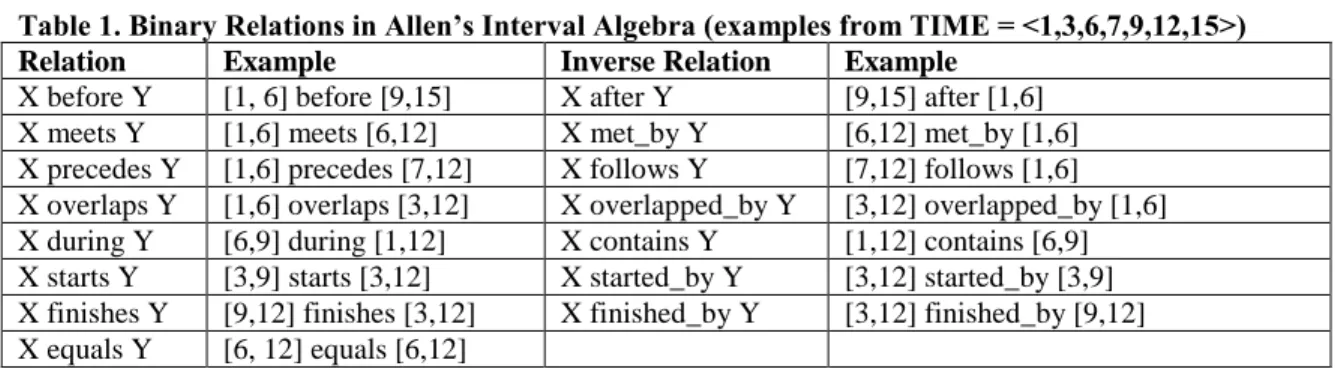
Table 1. Binary Relations in Allen’s Interval Algebra (examples from TIME = <1,3,6,7,9,12,15>)
Relation Example Inverse Relation Example
X before Y [1, 6] before [9,15] X after Y [9,15] after [1,6] X meets Y [1,6] meets [6,12] X met_by Y [6,12] met_by [1,6] X precedes Y [1,6] precedes [7,12] X follows Y [7,12] follows [1,6] X overlaps Y [1,6] overlaps [3,12] X overlapped_by Y [3,12] overlapped_by [1,6] X during Y [6,9] during [1,12] X contains Y [1,12] contains [6,9] X starts Y [3,9] starts [3,12] X started_by Y [3,12] started_by [3,9] X finishes Y [9,12] finishes [3,12] X finished_by Y [3,12] finished_by [9,12] X equals Y [6, 12] equals [6,12]
Definition. An interval algebra (IA) network [18] is a directed, vertex-labeled, edge-labeled graph G = (V, E, , ) where V and E are the set of vertices and edges, the vertex labeling function associates a Boolean formula Fi with each vertex vi in V and the edge labeling function :E2I associates a non-empty subset of the set I of relations in Allen’s interval algebra with each edge in E.
A vertex labeled with a Boolean condition p actually stands for some (unknown) closed time interval, denoted [[p]] = [xp, yp] having time instants xp and yp as its end-points, in which the condition p holds true (i.e., p is true at all time instants in the interval). If an edge from p to q is labeled with say {s, d, f, eq} then it is understood as a disjunction between the corresponding time intervals [[p]] and [[q]] i.e., [[p]] starts [[q]] [[p]] during [[q]] [[p]] finishes [[q]] [[p]] equal [[q]].
No two vertices are labeled by the same (or equivalent) condition. By convention, self-loops and parallel edges are not allowed and if we show the edge (i, j) then we do not show the inverse edge (j, i). If there is no edge between vertices p and q it means that we have no knowledge about the kind of relations that hold between the intervals [[p]] and [[q]]. An IA network specifies the relations that must hold between two intervals without specifying the actual end-points of the intervals.
Given an IA network G, a timeline TIME of timestamps and a temporal (time-stamped) database (a relation between TIME and records), we can compute the truth-value of each Boolean formula Fi in G at every instant in TIME, by means of a valuation function valFi:TIME {0,1}. For a Boolean formula F, we can then obtain a sequence of non-overlapping intervals IF = <I1, I2, …, Ik>, k 1, such that (i) truth-value of F is true at each instant in every Ii in IF, 1 i k; and (ii) F is not true at any time instant x in TIME if x does not belong to some interval Ij in IF; and (iii) Ii+1 is after Ii, for all 1 i k-1. Such a sequence of intervals IF is called the occurrence of F in TIME. Thus IF can be considered as a set of possible values (i.e., intervals) for the variable (i.e., vertex) vi; if F is false at all intervals then IF = .
Given an IA network G and a function that associates a domain of possible values IFi (i.e., set of possible intervals) with each vertex vi in G, an assignment is a function that assigns to every vertex vi in G some specific interval from the domain IFi of vi. An assignment for an IA network G is consistent if for every edge e in G, say between vertices vi and vj, there is one relation R in the edge label (e) of e ((e) I of the relations in Table 1) such that the intervals assigned to vi and vj “obey” R.
3.2 An Example
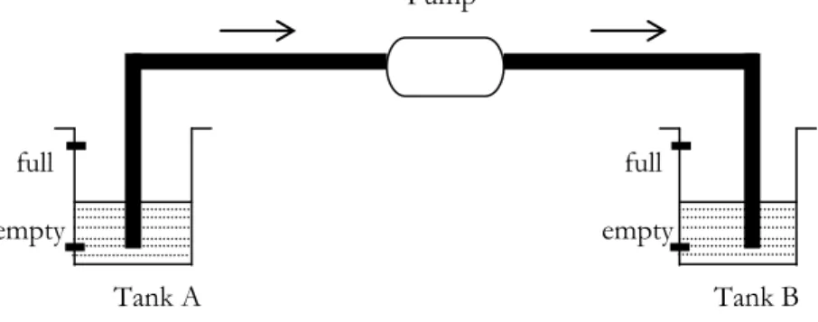
Consider a simple pumping control system (Figure 1) that transfers water from a source tank A into another sink tank B using a pump P. Each tank has a level-meter that measures the water level in the tank and sends it to the control system. Initially, both tanks are empty. The water level in either tank is an integer between 0 to 70 (say). Water level in a tank is empty when it is < 20, ok when it is 20 and 60 and it is full when it is > 60. The pump is to be switched on as soon as the water level in tank A reaches ok (from empty), provided that tank B is not full. The pump remains on as long tank A is not empty and as long as tank B is not full. The pump is to be switched off as soon as either the tank A becomes empty or tank B becomes full. The system should not attempt to switch the pump off (on), if it is already off (on). This example is simple but it can be extended to a controller for a complex network of pumps and pipes to control multiple source and sink tanks.
Pump
full full
empty empty
Tank A Tank B
Figure 1. A simple two tank pumping system.
The trace (log) of such a system can be a timestamped database having the following structure. timestamp pump_status water_level_a water_level_b
The timestamps are assumed to be sequential values 0, 1, 2, …. The pump_status can be 0 (pump is off) or 1 (pump is on). We introduce the following crisp Boolean propositions:
pump_on: is true when the pump is on
a_full, a_ok, a_empty: these are true respectively when the water level in tank A is high, ok or low b_full, b_ok, b_empty: these are true respectively when the water level in tank B is high, ok or low
Some patterns expected to be present in the “normal” trace of the system are:
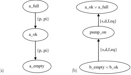
For tank A, full level can change only to ok level; ok level may change either to full or empty; empty level can only changes to ok. For tank A, this pattern is represented by the IA network in Figure 2(a). A similar pattern holds for tank B.
The pump remains on only when the water level in tank A is either ok or full and when the water level in tank B is either empty or ok. This pattern is represented by the IA network in Figure 2(b).
(a) (b)
Figure 2. IA networks to specify some patterns in the tank system.
We could have added some more relationships (i.e., edges) to the graph in Figure 2(b); e.g., an edge labeled with {p,b,pi,bi} between vertices (a_ok a_full) and a_empty. However, these relationships are not considered relevant for this pattern. Thus it is important to note that we do not care about the actual relationships that may hold between the vertices not connected by any edge. Suppose TIME = <0,1,2,3,4,5,6,7,8,9,10,11,12,13,14,15,16,17,18,19,20,21,22,23,24,25,26,27,28>. Suppose the intervals in which the various basic propositions are true (as obtained from some sample temporal database) are as follows: pump_on in [3,8], [13,21], a_full in [25,28], a_ok in [0,8], [11,24], a_empty is [9,10], b_full is [0,2],[13,21], b_ok in [3,12], b_empty in [22,28]. Then the intervals in which the formula associated with each vertex in Figure 2(b) is true in this timeline are as follows:
Variable Domain
u1 = a_full Iu1 = {[25,28]} u2 = a_ok Iu2 = {[0,8],[11,24]} u3 = a_empty Iu3 = {[9,10]} v1 = a_ok a_full IF1 = {[0,8], [11,28]} v2 = a_empty IF2 = {[9,10]} v3 = pump_on IF3 = {[3,8], [13,21]} v4 = b_empty b_ok IF4 = {[3,12], [22,28]} v5 = b_full IF5 = {[0,2], [13,21]}
3.3 Using Constraint Satisfaction for Detecting Pattern Defined by IA Network
The problem now is to select and assign an appropriate interval to each vertex such that the IA relationships associated with every edge label are obeyed. We map this temporal constraint satisfaction problem (TCSP) onto the classic constraint satisfaction problem (CSP) framework. Each vertex denotes an interval variable and its domain is given as a finite set of intervals, over each of which the associated Boolean proposition is true. Each IA relation can be neatly modeled as a constraint on a given pair of intervals and therefore each edge label represents a set of disjunctive constraints on the given pair of interval variables. Standard CSP techniques can now be used to solve this CSP problem. In general, we need all solutions of this TCSP problem (i.e., all consistent assignments of intervals that satisfy the given pattern specified by the IA network). Solving the TCSP problem is NP-complete [4], [18] and moreover, generating all solutions, is bound to be a harder task. On the positive side, available CSP engines internally implement sophisticated techniques for solving CSP problems. They are reported to have excellent performance against various benchmark CSP problems.
{s,d,f,eq} {s,d,f,eq} a_full
a_ok
a_empty {p, pi}
{p, pi}
a_ok a_full
pump_on
We use a particular CSP framework called constraint logic programming (CLP) which combines CSP with logic programming. Appendix A shows a program in CLP(FD) engine in GNU-Prolog that encodes the IA network of Figure 2(a) as a finite domain (FD) constraint satisfaction problem. Built-in CLP(FD) engine in GNU-Prolog solving for CSP over finite domains is invoked to solve the problem i.e., to assign the intervals to each vertex in the IA network, which is consistent with the edge constraints. The solution generated is {u1 ↦ [25,28], u2 ↦ [11,24], u3 ↦ [9,10]}. In general, there may be more than one solution, which can be obtained using backtracking in CLP(FD) system.
We have so far used crisp Boolean formulae to label the vertices in IA network to state crisp temporal patterns. Relations in IA are also crisp. In practice, to express uncertain and approximate patterns, we need “soft” patterns that use “soft” temporal relations between intervals where “soft” temporal propositions are strongly present. We now extend the IA network formalism for these.
4 The Temporal Constraints Diagram
4.1 Fuzzy Interval Algebra
Allen’s interval algebra provides 13 possible (crisp) binary relations between time intervals. There are several ways to fuzzify them. An obvious way is to treat each time interval as a fuzzy set subset of TIME whose degree of membership function is given by something like a trapezoidal function. Another approach can treat each time instant as a fuzzy number. The laws of fuzzy arithmetic can then be used to given a fuzzy semantics for the 13 binary operations in the algebra. We propose another way to fuzzify these relationships. Essentially, we keep the underlying intervals to be crisp and re-define each crisp binary relation in the algebra as a fuzzy binary relation over the set of all crisp intervals over TIME. Each such fuzzy binary relation associates a fuzzy degree of truth with a tuple of crisp intervals. The main idea behind our approach is to regard and as fuzzy connectives and to provide an appropriate fuzzification for the relational operators. By the well-known correspondence principle in fuzzy logic, we require that every such fuzzy binary relation should return a truth-value of 1 when the corresponding crisp relation holds between the given two intervals. For example, X fz_equals Y should be 1 when X equals Y. We can also suitably extend the semantics of these relations when either the first or second argument (but not both) is a time instant by considering an instant a as an interval [a,a]; e.g., a before [c,d] if a < c; a meets [c,d] if a+1 = c; a during [c,d] if a > c a < d; a after [c,d] if a > c etc.
We define parameterised fuzzy versions of the relational operators for positive integers (i.e., time instants, in our case). The crisp binary relation a < b is replaced by a fuzzy less than relation a ≺m b,
defined as follows: if a < b then a ≺m b = 1 else a≺m b = L(a,b-1,b+m), where the parameter m is a given positive integer constant. The L-membership function is shown in Figure 3(a). For example, 5 ≺3 6 = 1; 6≺3 6 = L(6,5,9) = 0.75; 7 ≺3 6 = 0.5. The crisp binary relation a = b is replaced by a
fuzzy equality relation a ≃m,n b, defined as follows: if a = b then a ≃m,n b = 1 else a ≃m,n b = (a,b-m,b,b+n), where the parameters m and n are given positive integer constants. The -membership function is shown in Figure 3(c); e.g., 6 ≃3,3 6 = 1; 5 ≃3,3 6 = (5,2,6,9) = 0.75; 7 ≃3,3 6 = 0.5. Other corresponding fuzzy relational operators are defined as follows, where we assume the standard fuzzy semantics for the logical connectives , , (i.e., t-norm is min and t-conorm is max).
a ≻m b =def (b≺m a)
a ≄m,n b =def (a≃m,n b)
Note that each of these fuzzy relations have an associated degree of membership function; e.g., the membership function for fuzzy greater than relation a >m b corresponds to the S-membership function in Figure 3(b). It is easy to verify some common laws that hold for the fuzzy relational connectives; e.g., a ≃m,n b = b ≃n,m a, for all a, b. Moreover, the relational operators always return 1 whenever the corresponding crisp relation holds between the arguments; e.g., a ≻m b = 1 whenever a > b.
L(x,,) = 1 if x S(x,,) = 0 if x (x,,,) = 0 if x = 0 if x = 1 if x = 0 if x = 1 – ((x - ) / ( - )) = (x - ) / ( - ) = (x-)/(-) if < x < = 1–((x-)/(-)) if <x<
(a) L membership (b) S membership (c) Triangle membership
Figure 3. Some common membership functions; x, , are time instants from TIME.
Table 2. Fuzzification of the Thirteen Relations in Allen’s Interval Algebra [a,b] fz_before [c,d] b ≺|d-b| c
[a,b] fz_meets [c,d] b+1 ≃b+1-a,d-c c
[a,b] fz_overlaps [c,d] (a ≺|d-a| c) (b ≻|d-b| c) (b ≺d-c d) [a,b] fz_during [c,d] (a ≻|d-a| c) (b ≺d-c d)
[a,b] fz_ starts[c,d] (b ≺d-c d) (a ≃|d-a|,|d-a| c)
[a,b] fz_finishes [c,d] (a ≽|d-a| c) (a ≺d-c d) (b ≃|b-c|,|b-c| d) [a,b] fz_equals [c,d] (a ≃|d-a|,|d-a| c) (b ≃|b-c|,|b-c| d)
[a,b] fz_after [c,d] [c,d] fz_before [a,b] [a,b] fz_met_by [c,d] [c,d] fz_meets [a,b]
[a,b] fz_overlapped_by [c,d] [c,d] fz_overlaps [a,b] [a,b] fz_contains [c,d] [c,d] fz_during [a,b]
[a,b] fz_started_by [c,d] [c,d] fz_starts [a,b] [a,b] fz_finished_by [c,d] [c,d] fz_finishes [a,b]
2, additional fuzzy binary relations between intervals can also be defined. For instance, we can compute the strength of overlap of two intervals [a,b] and [c,d] as:
[a,b] fz_overlaps1 [c,d] = (b-c) / (d-a) if [a,b] overlaps [c,d] or [a,b] finishes [c,d]
= 0 otherwise
Then, for example, [10,20] fz_overlaps1 [18,30] = (20 – 18) / (30-10) = 2/20 = 0.1 and [10,20] fz_overlaps1 [12,20] = (20-12) / (20-10) = 8/10 = 0.8. For both these examples, fz_overlap returns a value 1, since the given intervals do actually overlap.
4.2 Fuzzy Interval Algebra Network
There is a need to provide more facilities in the IA network notation in order to use it to specify complex patterns that appear in practical applications. The first such facility is to allow the user to specify a minimum length of the interval associated with any condition (vertex) in the IA network.
In addition, we need to allow soft conditions rather than crisp Boolean conditions. Thus one useful extension would be to allow a formula in fuzzy logic to be associated with a vertex. But then what is the meaning of the interval associated with a fuzzy logic formula? The fuzzy logic formula, say F, has a truth-value, at each instant in TIME, which is a real number in the closed interval [0, 1]. Thus given a fuzzy logic formula F and timeline TIME = <t0, t1, …, tN>, we get a valuation function valF : TIME [0,1]. In practical applications, we are often interested in finding one or all time intervals T of TIME such that F has a significant truth-value throughout T. When computing such time intervals for a given fuzzy logic formula F, we often wish to ignore local or short-term temporal variations in the truth-value of F and need to see “long-term” effects. One way to say that F has a significant presence in an interval T is to see whether F has an average truth-value in T which is at least as much as a desired threshold Q [0, 1]. The user can specify this by associating a threshold value Qi with each vertex vi in an IA network.
Thirdly, let IF and IG denote crisp maximally extended intervals for given fuzzy conditions F and G (for a given threshold Q). We now allow the use of fuzzy interval relations to hold between IF and IG. Let the set of shortened names of these relations be FI = {fz_b, fz_bi, fz_m, fz_mi, fz_p, fz_pi, fz_o, fz_oi, fz_d, fz_di, fz_s, fz_si, fz_f, fz_fi, fz_eq}. A fuzzy subset of FI associates a degree of truth with relations in FI; e.g., {fz_o:0.9, fz_eq:0.8}.
Definition. An extended interval algebra (EIA) network is a directed, vertex-labeled, edge-labeled graph G = (V, E, , , , ) where V and E are the set of vertices and edges, the vertex labeling function associates a fuzzy logic formula Fi, the threshold function :V[0,1] associates a threshold value with each vertex, a minimum duration function :VN associates a minimum interval length with the formula associates with each vertex and the edge labeling function associates a non-empty fuzzy subset of the set FI of fuzzy relations in Allen’s interval algebra with each edge in E.
For instance, in the example of section 3.2, suppose the trace included numeric measurement of the water level (in each tank) in say inches from the bottom of the tank, rather than a crisp classification of the water level into empty, ok and full. In such a case, we could define fuzzy propositions like high_a, low_a, high_b, low_b, increasing_a, decreasing_a, increasing_b, decreasing_b. Here, the fuzzy propositions high_a may denote how high the given level is in tank A. For instance if the minimum and maximum levels are 10 and 80 inches respectively for tank A, then the truth-value of the fuzzy proposition high_a could be defined as:
high_a = 0 if current level 20 inches = (current level – 20) / (60 – 20) if 20 current level 60
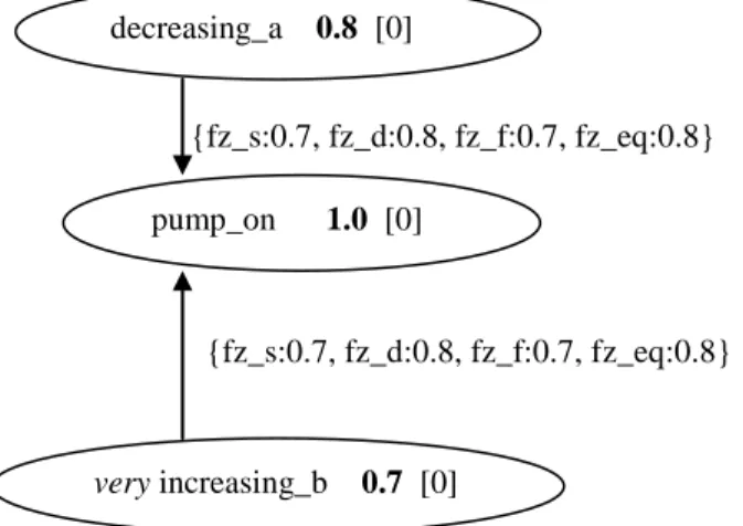
Truth-values of other fuzzy propositions can be similarly computed from the values in the trace. Using these fuzzy propositions we can define EIA networks to specify soft temporal patterns that can appear in the trace of the system. As an example, the pattern “whenever the pump is on, the water level in tank B increases rapidly and the water level in tank A decreases slowly” is specified using the EIA network in Figure 4. Here, very is a truth-qualifier; typically, very(x) =def x2 for x [0, 1]. The threshold is specified in bold. Since the minimum interval length are all specified as 0 (in square brackets), intervals of any length are acceptable. Since pump_on is a crisp Boolean variable, the threshold is set to 1.0
Figure 4. An EIA network for a soft temporal pattern in the pump system.
4.3 Semantics of EIA network
Given an EIA network G, a temporal database T and a timeline TIME of timestamps in T, we now define what it means to say that the pattern specified by G occurs in T in the interval say [x0, y0].
Let I = <ti, ti+1, …, ti+k> be an interval over TIME where each tj TIME, i j i+k. By (F, I), we denote the average value of F in the interval I i.e., (F, I) = ( valF(ti) + valF(ti+1) + … + valF(ti+k) ) / (k+1). Given a real number Q [0, 1], a fuzzy logic formula F and its valuation valF : TIME [0,1], a time interval I is said to be maximally extended if (F, I) Q and for any time interval I1 which properly contains I, (F, I1) < Q. Thus a maximally extended time interval I cannot be extended in any direction without reducing the average value of F below the given threshold.
Thus, given a time domain TIME, a threshold Q [0, 1], a fuzzy logic formula F and a valuation valF: TIME [0,1], we can obtain a sequence of non-overlapping intervals IF = <I1, I2, …, Ik>, k 1, such that (i) (F, Ii) Q, for all intervals Ii in IF, 1 i k; and (ii) each interval Ii in IF, 1 i k, is maximally extended; and (iii) Ii+1 is after Ii, for all 1 i k-1 [16, 17]. Such a sequence of intervals IF is called an occurrence of F in TIME. Thus, given an EIA network G, we can construct the occurrence (i.e., an ordered sequence of intervals in TIME) IFi for each vertex vi in G, which satisfies the above 3 criteria. Clearly, an occurrence IF is not unique. Depending on the strategy used in an algorithm to compute an occurrence, there can be many different sequences of maximally separated intervals that satisfy the above definition; see [14] for one possible algorithm to compute an occurrence. Whether any particular choice of occurrence is better or more intuitive is an important question that we have not addressed here. In our experience, the occurrence computed by the algorithm in [14] closely matches user’s expectations.
{fz_s:0.7, fz_d:0.8, fz_f:0.7, fz_eq:0.8} {fz_s:0.7, fz_d:0.8, fz_f:0.7, fz_eq:0.8} decreasing_a 0.8 [0]
pump_on 1.0 [0]
Given an EIA network G and a function that associates an occurrence (i.e., a sequence of intervals in TIME) with each vertex in G, an assignment is a function that assigns to every vertex vi in G some specific interval from the set of occurrences IFi of the fuzzy logic formula Fi associated with vi. Thus the sequence of intervals IFi forms a domain of possible values for the “variable” vi. An assignment for an EIA network G is consistent if for every edge e in G, say between vertices vi and vj, there is one relation R having degree of membership w in the edge label X of e (X is a subset of the fuzzy binary interval relations from Table 2) such that the degree of relation R for intervals assigned to vi and vj is at least w.
4.2 Using Constraint Satisfaction to Detect Pattern Defined by EIA Network
As in section 3.3, the constraint satisfaction framework can be used for the pattern detection task. Each vertex (i.e., a formula F in fuzzy logic) denotes an interval variable and its domain is given as a finite set of intervals, over each of which the associated fuzzy formula is present with the required strength and the interval has the minimum specified length. Each fuzzy IA relation (Table 2) can be neatly modeled as a constraint on a given pair of intervals and therefore each edge label represents a set of disjunctive constraints on the given pair of interval variables. Standard CSP techniques can now be used to solve this CSP problem. We have used the particular CLP framework in GNU-Prolog for solving this finite domain CSP problem. The details are similar to Appendix A.
5 Conclusions and Further Work
We presented an enhanced interval algebra network notation along with its semantics and advocated its use as a simple visual mechanism for specifying soft temporal patterns. The basic idea behind this extension is to associate (non-temporal) crisp or fuzzy logic formulae with each vertex of the IA network, which facilitates specification of soft temporal patterns. We also proposed minimum duration and minimum average strength as additional facilities in the EIA notation. We defined and used fuzzy interval algebra relations for disjunctive constraints on edges in EIA network. We formulated the problem of detecting the pattern defined by the given EIA network as a finite domain constraint satisfaction problem. We used a constraint logic programming engine CLP(FD) in GNU-Prolog to solve this problem. We illustrated the approach with the example of a dynamic process control system.
Apart from providing a new way of specifying soft temporal patterns, another novel aspect of our approach is that it ties the task of detecting a temporal pattern with the problem of temporal constraint satisfaction, which is being heavily researched in the AI literature. It is hoped that AI techniques from temporal constraint satisfaction community can then be fruitfully used for pattern detection.
Further exploration of this approach involves support for higher level patterns which are either Boolean combinations of EIA networks or hierarchical EIA networks, where each vertex may itself refer to a “lower-level” EIA network. We also need to investigate if any graph-theoretic and temporal logic-based techniques can be applied to transform the given EIA network to an equivalent but simpler one. We are also looking at the problem of learning or generating an EIA network from a given temporal database i.e., the classical problem of recognition of temporal patterns (represented here as EIA networks) in given temporal databases.
Acknowledgements.
References
[1] Allen J.F., 1984. Towards a General Theory of Action and Time. Artificial Intelligence, 23(2), pp. 123-154.
[2] S. Badaloni, M. Giacomin, 2000. A Fuzzy Extension of Allen’s Interval Algebra. in E. Lamma, P. Mello, (ed.s), Proc. AI*IA99, LNAI 1792, pp. 155-165, Springer-Verlag, 2000.
[3] Brusoni V., Console L., Terenziani P., Pernici B., 1999. Qualitative and Quantitative Constraints and Relational Databases: Theory, Architecture and Applications. IEEE Trans. Knowledge Data Engg., vol. 11, no. 6, Nov-Dec., 1999, pp. 948-968.
[4] Dechter R., Meiri I., Pearl J., 1991. Temporal Constraint Networks. Artificial Intelligence, 49 (1991), pp. 61-95.
[5] Faloutos C., Ranganathan M., Manolopoulous Y., 1994. Fast Sub-sequence Matching in Time Series Database. Proc. 1994 ACM SIGMOD, 1994.
[6] Fu K.S., 1982. Syntactic Pattern Recognition and Applications. Prentice-Hall, 1982.
[7] J.W. Guesgen, J. Hertzberg, A. Philpott, 1994. Towards Implementing Fuzzy Allen Relations. Proc. ECAI-94 Workshop on Spatial and Temporal Reasoning, pp. 49-55, 1994.
[8] Inmon W.H., Osterfelt S., 1991. Understanding Data Pattern Processing. QED Technical Publishing Group, 1991.
[9] Kartalopoulos S.V., 2000. Understanding Neural Networks and Fuzzy Logic. Prentice-Hall, 2000.
[10]Kennedy R.L., Lee Y., Roy B.V., Reed C.P., Lippman R.P., 1998. Solving Data Mining Problems Through Pattern Recognition. Prentice-Hall PTR, 1998.
[11]Kirkland J.D., Senator T.E., Hayden J.J., Dybala T., Goldberg H.G., Shyr P., 1999. The NASD Regulation Advanced Detection System (ADS). Proc. Spring 1999 AAAI Conf., pp. 55-67. [12]Maidchhi R., Pernici B., Barbie F., 1992. Automatic Deduction of Temporal Information. ACM
Trans. Database Systems, Vol. 17, No. 4, Dec. 1992, pp. 647-688.
[13]Miguel I., Shen Q., 2001. Solution Techniques for Constraint Satisfaction Problems: Foundations and Advanced Approaches. AI Review, vol. 15, no. 4, June 2001, pp. 243-293.
[14]Palshikar G. K., 2001. A Fuzzy Temporal Notation and Its Applications to Specify Fault Patterns for Diagnosis. Pattern Recognition Letters, vol. 22, no. 3-4, March 2001, pp. 381-394. [15]Palshikar G.K., 2000. Representing Fuzzy Temporal Knowledge. Int. Conf. Knowledge-Based
System (KBCS-2000), Allied Publishers, pp. 252-263.
[16]Rasmussen D., Yager R.R., 1997. A Fuzzy SQL Summary Language for Data Discovery. In Fuzzy Information Engg., D. Dubois, H. Prade, R.R. Yager (eds), John Wiley, 1997, pp. 253-264. [17]Shimakawa H., Kikkawa K., 1992. Trend Recognition with Time Series Database. Proc. 2nd Far
East Workshop on Future Datasbase Systems (Future Databases ’92), World Scientific, 1992. [18]P. van Beek, 1992. Reasoning about Qualitative Temporal Information. Artificial Intelligence, 58
(1992), pp. 297-326.
APPENDIX A. GNU-Prolog Finite Domain CSP Program for Figure 2(a).
fig_2a :-
fd_set_vector_max(70),
LD = [X0, X1, Y0, Y1, Z0, Z1], /*end-points of intervals as variables */ fd_domain(LD,0,70),
fd_relation([[25,28]], [X0,X1]), /* a_full intervals [25,28] */
fd_relation([[0,8],[11,24]], [Y0,Y1]), /* a_ok intervals [0,8], [11,24] */ fd_relation([[9,10]], [Z0,Z1]), /* a_empty intervals [9,10] */
/* enforce interval end point constaints */
interval_end_point_constraint([[X0,X1],[Y0,Y1],[Z0,Z1]]),
/* constraint on edge from a_full to a_ok */ ( edge_constraint1([X0,X1],[Y0,Y1],precedes) ; edge_constraint1([X0,X1],[Y0,Y1],preceded_by) ),
/* constraint on edge from a_ok to a_empty */ ( edge_constraint1([Y0,Y1],[Z0,Z1],precedes) ; edge_constraint1([Y0,Y1],[Z0,Z1],preceded_by) ),
fd_labeling(LD), /* call CSP engine to solve */ write('Solution: '), write(LD), nl.
interval_end_point_constraint([]).
interval_end_point_constraint([[X0,X1] | T]) :- X1 #>= X0,
interval_end_point_constraint(T).
/* Encode IA relations as constraints over intervals */
/* edge_constraint1([SrcInt0,SrcInt1],[DestInt0,DestInt1],RelationName) */ edge_constraint1([X0,X1],[Y0,Y1],before) :- Y0 #> (X1 + 1).
edge_constraint1([X0,X1],[Y0,Y1],after) :- edge_constraint1([Y0,Y1],[X0,X1],before).
edge_constraint1([X0,X1],[Y0,Y1],meets) :- X1 #= Y0. edge_constraint1([X0,X1],[Y0,Y1],met_by) :-
edge_constraint1([Y0,Y1],[X0,X1],meets).
edge_constraint1([X0,X1],[Y0,Y1],precedes) :- Y0 #= (X1 + 1). edge_constraint1([X0,X1],[Y0,Y1],preceded_by) :-
edge_constraint1([Y0,Y1],[X0,X1],precedes).
edge_constraint1([X0,X1],[Y0,Y1],overlaps) :- X1 #> Y0, X1 #< Y1. edge_constraint1([X0,X1],[Y0,Y1],overlapped_by) :-
edge_constraint1([Y0,Y1],[X0,X1],overlaps). edge_constraint1([X0,X1],[Y0,Y1],during) :- X0 #> Y0, X0 #< Y1,
X1 #> Y0, X1 #< Y1.
edge_constraint1([X0,X1],[Y0,Y1],contains) :- edge_constraint1([Y0,Y1],[X0,X1],during).
edge_constraint1([X0,X1],[Y0,Y1],starts) :- X0 #= Y0, X1 #< Y1. edge_constraint1([X0,X1],[Y0,Y1],started_by) :-
edge_constraint1([Y0,Y1],[X0,X1],starts). edge_constraint1([X0,X1],[Y0,Y1],finishes) :- X1 #= Y1, X0 #> Y0, X0 #< Y1.
![Table 2. Fuzzification of the Thirteen Relations in Allen’s Interval Algebra [a,b] fz_before [c,d] b ≺ |d-b| c](https://thumb-us.123doks.com/thumbv2/123dok_us/8195712.2172688/7.918.132.795.272.536/table-fuzzification-thirteen-relations-allen-interval-algebra-before.webp)