Chap5 - Gaits and Cyclic Motion

(1)

Chapter 5:

Gaits and Cyclic Motion

(2)

Motion planning

(3)

Motion Planning

Given the local connection, could we just define a path through

the world, and then use

(4)

Motion Planning

Inverse kinematics not always sufficient:

2. Singularities, Sinks, and Joint limits: what’s wrong with these?

1. Constrained directions – only

certain paths are admissible

Aξx

Figure 3.1: Connection vectorﬁelds for the three-link kinematic snake shown in Table. 2.1. TheAξy ﬁ_eld

is null at all points in the shape space, as the middle wheelset constrainsξy to zero under all conditions.

Due to singularities in the vectorﬁelds at the linesα1=±π, α2=±π, andα1=α2, the magnitudes of

the vectorﬁelds have been scaled by their arctangents for readability. The input shape vectors ataand

bproduce pure forward translation and pure negative rotation, respectively.

3.2 Examples

Beyond allowing for characterization of the effect of input shape velocities, the connection vector ﬁelds also facilitate decomposing the displacements caused by shape changes and gaits into their constituent motions, as demonstrated in the examples below.

3.2.1 F loating Snake

As the ﬁrst two rows of the ﬂoating snake’s local connection in (2.10) are null, all the information regardingthesystem’sposition changein responsetoashapechangeisencoded in the third, rotational row of the local connection. The plot of Aξθ, the corresponding

connection vector ﬁeld, in Fig. 3.2(a) matches an intuitive understanding of how a system governed by conservation of angular momentum should behave: the general trend to point in the +α1, −α2 direction corresponds to the central body counterrotating against the

outer links. The exact heading of the ﬁeld varies with how much leverage the links exert on the system; the more extended an outer link is, the more the central body needs to counter-rotate to nullify the outer link’s angular momentum.

29

Kinematic snake can’t pass through singularities at “C” shapes Three-link swimmer can’t move laterally from this shape

(5)

Motion Planning

• _{Full optimal control requires solving whole path}

at once (respecting constraints, limits, etc.)

• _{Maneuver-based planning precalculates short}

paths that

1. Avoid joint limits and singularities

2. Displace the system in some “useful” manner

3. Can be concatenated together to form a

(6)

Gaits

Gaits are

cyclic

motions in the shape space

(7)

Nonconservativity and Noncommutativity

Kinematic gaits operate on two basic principles:

• _{Nonconservatvity: System pulls itself forward}

more than it pushes itself backward each cycle

• _{Noncommutativity: System rotates during the}

(8)

Nonconservativity Example

(9)

Stokes’s Theorem

(vector calculus version)

(10)

Curl

Curl is sometimes described as “how

much the vector field is ‘rotating’

around a point”

Magnitude also comes in

here, so this description

can be somewhat

confusing

Another way to think of it is “the

derivatives of the vector components

along orthogonal directions in the

space”

(11)

Curl and the Floating Snake

–

+

(12)

Gaits and Stokes’s theorem

Walsh and Sastry, 1995

(13)

(14)

(15)

(16)

(17)

(18)

(19)

Displacement

(20)

Available

coordinate choices?

Good

coordinate choice?

(21)

Noncommutativity

Car cannot move sideways, but,

because translations and rotations

do not commute, it can “parallel

park” to get a net lateral motion

curl

(22)

Lie Brackets

Lie bracket measures how vector fields change along each other

Lie bracket

Directional derivative

of Y along X

Directional derivative

of X along Y

Output of the Lie bracket of two vector fields is a vector field. At each point,

differentially flowing along X, Y, -X, and –Y (in order) is equivalent to flowing along

[X,Y] for equal time

NONCONSERVAT IVIT Y AND NONCOMMUTAT IVIT Y IN LOCOMOT ION

7 There are several applications of the Lie bracket in the context of control systems, but the

interpretation most germane to the present work is that

ﬂ

owing differentially along

X

,

Y

,

−

X

, and

−

Y

is equivalent to

ﬂ

owing differentially along [

X, Y

].

A special deﬁ

nition of the Lie bracket applies to elements of the Lie algebra

g

corresponding

to a Lie group

G

. In this case, the Lie bracket of two vectors

u, v

∈

g

is the Lie bracket of the

two

left-invariant

vector

ﬁ

elds on

_G

generated by applying the left lifted action to

_u

and

_v

,

[

_{u, v}

]

≡

[

_T

_e

_L

_g

_{u, T}

_e

_L

_g

_v

]

_g=e

_.

(3.5)

Hodge-Helmholtz decomposition.

The fundamental theorem of calculus states that for a

one-dimensional function, if we know

_dy/dx

as a function of

_x

, then we know

_y

(

_x

) up to a

constant of integration. Expansions of this principle to higher dimensions lead to the

fun-damental theorem of vector calculus, which, among other results, states that if we know the

gradient of a function, we know the function up to the addition of a scalar, and that if we

know the curl of a vector

ﬁ

eld, we know the vector

ﬁ

eld up to the addition of a gradient

(conservative)

ﬁ

eld. In terms of differential forms, both these statements are aspects of a

more general theorem that states that if we know the exterior derivative

dω

of a form

ω

, then

we know

ω

up to the addition of a closed form.

In single-variable calculus, many functions have canonical anti-derivatives, such as

´

cos =

sin, to which the constant of integration is added. Similarly, it is often useful to designate

a core form

Ω

as the anti-exterior-derivative of a form

ω

. This separation is achieved by

the

Hodge decomposition

[

3 ], referred to as the

Helmholtz decomposition

in vector calculus

contexts. The Hodge-Helmholtz decomposition splits a

k

-form

ω

into three components,

ω

=

d

A

+

δ

B

+

C

,

(3.6)

where

d

A

is an exact, and therefore closed,

k

-form (corresponding to a curl-free vector

ﬁ

eld),

δ

_B

is a

_k

-form orthogonal to the set of closed

_k

-forms (a divergence-free

ﬁ

eld in vector calculus),

and

C

is a

harmonic remainder

(satisfying boundary conditions), generally much smaller than

either of the

ﬁ

rst two components. Drawing on the properties that

d(d

A

) = 0 and that the

exterior derivative is a linear operator, we can see that as

dω

=

d(δ

B

+

C

)

_,

(3.7)

dω

is unaffected by the choice of

A

and that

d

A

thus acts similarly to a constant of integration

when determining

ω

from

dω

.

The

d

A

term is the projection of

ω

onto the space of conservative

_k

-forms. For one-forms,

the sum

δ

B

+

C

therefore has the interesting property of being the

smallest

one-form with an

exterior derivative equal to that of

ω

,

argmin

dω =dω

(

´

Ω

ω

2 ) =

ω− d

A

=

δ

B

+

C

,

(3.8)

where the

“size”

of

ω

is its squared norm integrated over the domain. In [

13 ,

14 ], we

demon-strated a useful correspondence between this sum (which, due to the relatively small

contribu-tion of

C

, we refer to as the

“divergence free component”

for brevity) and an optimal choice of

coordinates for locomotion analysis, and presented a numerical algorithm for

ﬁ

nding it over a

ni

ﬁ

te domain, based on that in [

9 ]. In

§

6 , we examine this application more closely, and from

a differential geometric standpoint.

When we have a Lie group, we can talk about the Lie bracket of two vectors

u,v

in

T

_e

G

as

meaning the Lie bracket of their left-invariant fields, evaluated at the origin

(23)

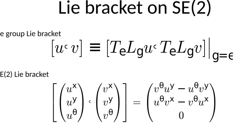
Lie bracket on SE(2)

NONCONSERVAT IVIT Y AND NONCOMMUTAT IVIT Y IN LOCOMOT ION

7 There are several applications of the Lie bracket in the context of control systems, but the

interpretation most germane to the present work is that

ﬂ

owing differentially along

X

,

Y

,

−

X

, and

−

_Y

is equivalent to

ﬂ

owing differentially along [

_{X, Y}

].

A special deﬁ

nition of the Lie bracket applies to elements of the Lie algebra

g

corresponding

to a Lie group

G

. In this case, the Lie bracket of two vectors

u, v

∈

g

is the Lie bracket of the

two

left-invariant

vector

ﬁ

elds on

_G

generated by applying the left lifted action to

_u

and

_v

,

[

_{u, v}

]

≡

[

_T

_e

_L

_g

_{u, T}

_e

_L

_g

_v

]

_g=e

_.

(3.5)

Hodge-Helmholtz decomposition.

The fundamental theorem of calculus states that for a

one-dimensional function, if we know

dy/dx

as a function of

x

, then we know

y

(

x

) up to a

constant of integration. Expansions of this principle to higher dimensions lead to the

fun-damental theorem of vector calculus, which, among other results, states that if we know the

gradient of a function, we know the function up to the addition of a scalar, and that if we

know the curl of a vector

ﬁ

eld, we know the vector

ﬁ

eld up to the addition of a gradient

(conservative)

ﬁ

eld. In terms of differential forms, both these statements are aspects of a

more general theorem that states that if we know the exterior derivative

dω

of a form

ω

, then

we know

ω

up to the addition of a closed form.

In single-variable calculus, many functions have canonical anti-derivatives, such as

´

cos =

sin, to which the constant of integration is added. Similarly, it is often useful to designate

a core form

Ω

as the anti-exterior-derivative of a form

ω

. This separation is achieved by

the

Hodge decomposition

[

3 ], referred to as the

Helmholtz decomposition

in vector calculus

contexts. The Hodge-Helmholtz decomposition splits a

_k

-form

ω

into three components,

ω

=

d

A

+

δ

B

+

C

,

(3.6)

where

d

A

is an exact, and therefore closed,

k

-form (corresponding to a curl-free vector

ﬁ

eld),

δ

_B

is a

_k

-form orthogonal to the set of closed

_k

-forms (a divergence-free

ﬁ

eld in vector calculus),

and

C

is a

harmonic remainder

(satisfying boundary conditions), generally much smaller than

either of the

ﬁ

rst two components. Drawing on the properties that

d

(

d

A

) = 0 and that the

exterior derivative is a linear operator, we can see that as

dω

=

d

(

δ

B

+

C

)

_,

(3.7)

dω

is unaffected by the choice of

A

and that

d

A

thus acts similarly to a constant of integration

when determining

ω

from

dω

.

The

d

A

term is the projection of

ω

onto the space of conservative

_k

-forms. For one-forms,

the sum

δ

B

+

C

therefore has the interesting property of being the

smallest

one-form with an

exterior derivative equal to that of

ω

,

argmin

dω =dω

(

´

Ω

ω

2 ) =

ω− d

A

=

δ

B

+

C

,

(3.8)

where the

“

size

”

of

ω

is its squared norm integrated over the domain. In [

13 ,

14 ], we

demon-strated a useful correspondence between this sum (which, due to the relatively small

contribu-tion of

C

, we refer to as the

“

divergence free component

”

for brevity) and an optimal choice of

coordinates for locomotion analysis, and presented a numerical algorithm for

ﬁ

nding it over a

ni

ﬁ

te domain, based on that in [

9 ]. In

§

6 , we examine this application more closely, and from

a differential geometric standpoint.

10 ROSS L. HAT T ON AND HOWIE CHOSET

(a) World velocity

(b) Body velocity

(c) Alternate

interpreta-tion of body velocity

Figure4.1: T hreerepresentations of thevelocity of a robot. T herobot, represented by thetriangle, is translating

up and to the right while spinning counterclockwise. In

(a)

, the world velocity, ˙

g, is measured with respect

to the global frame. T he body velocity, ξ, in

(b)

is the velocity represented in the robot’s instantaneous local

coordinate frame. T he body velocity is actually calculated by transporting the body back to the origin frame,

as in

(c)

, but by symmetry this is equivalent to bringing the world frame to the system.

Table 4.1: Interpretations of elements of T

e

G, as used in this paper.

Symbol

Meaning

First Introduced

ξ

Body velocity

_§

4.1 z

Exponential coordinates

§

4.1 ζ

Body velocity integral

§

5.2.1 ¯

ζ

Corrected body velocity integral

_§

5.2.2 g

= exp (

z

) of a vector

z

∈

se

(2)

ﬁ

nds the net displacement of a system starting at the origin

and moving with body velocity

ξ

=

z

for one unit of time, and takes the form

(

x, y

) =

(

z

x

, z

y

)

,

for

z

θ

= 0

1 z

θ

sin

z

θ

1 −

cos

z

θ

cos

z

θ

−

1 sin

z

θ

z

x

z

y

,

for

z

θ

_{= 0}

θ

=

z

θ

.

(4.5)

The elements of

z

are the

exponential coordinates

corresponding to

g

. Note that both the body

velocity and exponential coordinates are elements of the tangent space of the body frame,

but have different physical interpretations. In the following discussion, we will maintain the

orthographic distinction between these quantities, summarized in Table

4.1 , adding two more

interpretations in

§

5.2 .

The Lie bracket of two vectors

u, v

∈

se

(2) for an

SE

(2) system

ﬁ

nds the net effect of

moving differentially in the

u, v,

−

u,

−

v

directions and is calculated as

u

x

u

y

u

θ

,

v

x

v

y

v

θ

=

v

θ

u

y

−

u

θ

v

y

u

θ

v

x

−

v

θ

u

x

0 ,

(4.6)

Lie group Lie bracket

(24)

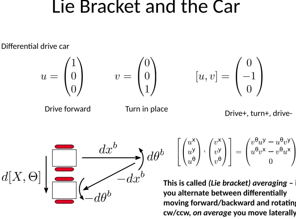
Lie Bracket and the Car

Differential drive car

Drive forward

Turn in place

_{Drive+, turn+,}

drive-10 ROSS L. HAT T ON AND HOWIE CHOSET

(a) World velocity (b) Body velocity (c) Alternate interpreta-tion of body velocity

Figure4.1: T hreerepresentations of thevelocity of a robot. T herobot, represented by thetriangle, is translating up and to the right while spinning counterclockwise. In (a), the world velocity, ˙g, is measured with respect to the global frame. T he body velocity, ξ, in (b) is the velocity represented in the robot’s instantaneous local coordinate frame. T he body velocity is actually calculated by transporting the body back to the origin frame, as in(c), but by symmetry this is equivalent to bringing the world frame to the system.

Table 4.1: Interpretations of elements of TeG, as used in this paper.

Symbol

Meaning

First Introduced

ξ

Body velocity

_§

4.1 z

Exponential coordinates

_§

4.1 ζ

Body velocity integral

_§

5.2.1 ¯

ζ

Corrected body velocity integral

_§

5.2.2 g

= exp (

z

) of a vector

z

∈

se

(2)

ﬁ

nds the net displacement of a system starting at the origin

and moving with body velocity

ξ

=

z

for one unit of time, and takes the form

(

x, y

) =

θ

1 −

cos

z

θ

cos

z

θ

−

1 sin

=

z

θ

.

(4.5)

The elements of

z

are the

exponential coordinates

corresponding to

g

. Note that both the body

velocity and exponential coordinates are elements of the tangent space of the body frame,

but have different physical interpretations. In the following discussion, we will maintain the

orthographic distinction between these quantities, summarized in Table

4.1 , adding two more

interpretations in

_§

5.2 .

The Lie bracket of two vectors

u, v

∈

se

(2) for an

SE

(2) system

ﬁ

nds the net effect of

moving differentially in the

u, v,

−

u,

0 ,

(4.6)

(25)

1 . Controlability:

DO WE WANT TO MORE FORMALLY DEFINE CONTROLLABILITY AND/OR ITS RELATIVES

ON THE NEXT SLIDE?

Nonholonomically-constrained systems by definition cannot instantaneously move

in some directions: their distributions do not span their configuration spaces

If we take a distribution

DID WE DEFINE A DISTRIBUTION YET? PERHAPS WE SHOULD REMIND PEOPLE

HERE

D={V

₁

,V

₂

}

AN OSCILLATION BUT PERHAPS JUST SPOKEN WORDS IS ENOUGH

of the controls. In some cases, we can

further expand the distribution with higher-order Lie brackets, e.g.,

can’t add dimensions

–

YOU MEAN REACH THE FULL DIMENSION

by taking

more Lie brackets, this is an

involutive distribution

: it describes the full set of directions in which the

system can move differentially. If a system’s involutive distribution spans the whole configuration space,

then the system is said to be

controllable

– we have a set of inputs that can move the system in any

direction. (Note that in general there will be more efficient/effective ways to move the system in

non-primary directions, controllability is a proof of existence)

(26)

2. Relationship to gaits.

Importance of Lie brackets

are associated with unit shape velocities,

and so their Lie bracket corresponds to the

motion produced by a differential

oscillation in the shape space (i.e. a

differential gait)

(27)

Lie Bracket and Larger Motions

One of the nice things about thinking of Lie

bracket motions as differential gaits is that it

gives us intuition as to how the system will move

over larger gaits: Two differential cycles are

equivalent to their combined perimeter if the

overlapping edges cancel out.

This gives us an area rule: over a larger gait,

magnitude of average flow field is the area

integral of the Lie bracket over the region

enclosed by the gait –

I FEEL AREA COMES OUT

OF NOWHERE? Why can we talk about area?

Note that here there is a small-angle condition on this assumption, and we are also assuming that local connection is constant (and thus that input fields are left invariant) – EXPLAIN LOCAL

CONNECTION IS CONSTANT

10 ROSS L. HAT T ON AND HOWIE CHOSET

(a) World velocity (b) Body velocity (c) Alternate interpreta-tion of body velocity

Figure4.1: T hreerepresentations of thevelocity of a robot. T herobot, represented by thetriangle, is translating up and to the right while spinning counterclockwise. In (a), the world velocity, ˙g, is measured with respect to the global frame. T he body velocity, ξ, in (b) is the velocity represented in the robot’s instantaneous local coordinate frame. T he body velocity is actually calculated by transporting the body back to the origin frame, as in (c), but by symmetry this is equivalent to bringing the world frame to the system.

Table 4.1: Interpretations of elements of TeG, as used in this paper.

Symbol

Meaning

First Introduced

ξ

Body velocity

_§

4.1 z

Exponential coordinates

_§

4.1 ζ

Body velocity integral

_§

5.2.1 ¯

ζ

Corrected body velocity integral

_§

5.2.2 g

= exp (

z

) of a vector

z

∈

se

(2)

ﬁ

nds the net displacement of a system starting at the origin

and moving with body velocity

ξ

=

z

for one unit of time, and takes the form

(

x, y

) =

θ

1 −

cos

z

θ

cos

z

θ

−

1 sin

=

z

θ

.

(4.5)

The elements of

z

are the

exponential coordinates

corresponding to

g

. Note that both the body

velocity and exponential coordinates are elements of the tangent space of the body frame,

but have different physical interpretations. In the following discussion, we will maintain the

orthographic distinction between these quantities, summarized in Table

4.1 , adding two more

interpretations in

_§

5.2 .

The Lie bracket of two vectors

u, v

∈

se

(2) for an

SE

(2) system

ﬁ

nds the net effect of

moving differentially in the

u, v,

−

u,

0 ,

(4.6)

This rule is consistent with the Lie

bracket as a

bilinear operator

– it

scales linearly with

u

and

v.

Example: Increasing forward translation and rotation each linearly increases the lateral translation

(28)

Lie Brackets and Exponential Maps

Lie bracket gives us average velocity of the system: moving for dt along each of

u, v

,

-u

, and

-v

is equivalent to moving for dt along [u,v]. (note that the total “time” in

the cycle is different from the “flow time” along the Lie bracket field).

To get the

displacement

over the cycle, we can exponentiate this

velocity:

CAN YOU REMIND ME AGAIN WHEN THE EXPONENTIAL

IS RELATED TO A GROUP OPERATOR; IS THIS TRUE FOR ALL LIE

GROUPS, IE IS THE DEFINING FEATUER OF LIE GROUPS

Here, [

u,v

]

dt

gives the

exponential coordinates

of the net displacement, In the future, we will

denote such exponential coordinates as

z

.

Also note that if we scale

u

or

v

, we proportionally increase the displacement

(29)

Nonconservativity

_{Noncommutatvity}

6 ROSS L. HAT T ON AND HOWIE CHOSET

Where necessary,

musical notation

[

1 ] is used to denote the relationship between

k

-forms

and their vector-calculus duals, with

ω

=

v

representing a conversion from a one-form to a

vector

ﬁ

eld, and

v

=

ω

the conversion from vectors to one-forms. Similarly, the

Hodge star

operator provides the mathematical structure for representing a differential area (a two-form)

by its normal vector (a one-form), as (

∗ω

) .

The

exterior derivative dω

of a

k

-form

ω

measures how each component of

ω

changes in

directions normal to that component, and is itself a

k

+1-form. For the examples we consider in

this paper, which are restricted to

k

-forms over two-dimensional spaces, the exterior derivative

is intuitively linked to two common vector operations

–

gradient and curl. The gradient vector

e

ﬁ

ld of a function (zero-form) is the dual to the function

’

s exterior derivative; likewise, the

curl of a two-dimensional vector

ﬁ

eld is the corresponding one-form

’

s exterior derivative.

2 Two important classi

ﬁ

cations of differential forms are

closed

and

exact

. Closed forms have

null exterior derivatives,

dω

= 0, and exact forms are themselves the exterior derivatives of

other forms,

ω

=

dω

_a

. An especially useful result from differential geometry [

1 ] is that exact

forms are automatically closed,

d

(

dω

) = 0, which is equivalent to saying that the curl of a

gradient

ﬁ

eld is always zero (and thus that gradient

ﬁ

elds are conservative). We will return

to this point in our discussion of optimal coordinates.

Stokes’s theorem.

Stokes

’

s theorem [

6 ] equates the integral of a differential

k

-form

ω

along

a closed

k

-dimensional manifold

∂Ω

on a space

U

to the integral of the exterior derivative of

that

k

-form over a

k

+ 1-dimensional manifold

Ω

bounded by the original manifold,

ˆ

∂Ω

ω

(

u

)

du

=

ˆ

Ω

dω

(

u

)

du.

(3.1)

In two dimensions and with

ω

a one-form, the surface

Ω

is simply the region of

U

enclosed

by the closed curve

∂Ω

, and (

3.1 ) specializes to the simple area integral

‰

∂Ω

ω

(

u

)

du

=

¨

Ω

∂ω

₂

∂

u

1 −

∂ω

₁

∂

u

2 du

1 _du

2 _.

_(3.2)

This equation is commonly encountered as

“

Green

’

s theorem

”

in vector calculus, where it is

described as equating a line integral along a closed loop on a vector

ﬁ

eld with an area integral

of the

ﬁ

eld

’

s curl.

Lie bracket of vector ﬁelds.

The Lie bracket [

29 ] of two vector

ﬁ

elds

X

and

Y

measures

their rates of change with respect to each other. For

ﬁ

elds de ne

ﬁ

d on an

n

-dimensional space

U

, the Lie bracket is a vector

ﬁ

eld de

ﬁ

ned as

[

X, Y

] = (

∇

Y

_·

X

)

−

(

∇

X

_·

Y

)

,

(3.3)

or componentwise as

[

X, Y

]

i

=

n

j =1

x

j

∂

y

i

∂

u

j

−

y

j

∂

x

i

∂

u

j

=

−

[

Y, X

]

i

_.

_(3.4)

2

_{In three dimensions, the exterior derivative has three magnitude components, corresponding to a}

three-dimensional curl vector ﬁeld (created via the Hodge star operator). In four or more dimensions, the number of

components in the exterior derivative continue to grow as (n

2

− n)/ 2, even though the curl is undeﬁned. T hese

cases are, however, outside the scope of the present work.

–

+

curl

(30)

Combining Nonconservativity and

Noncommutativity

Example: Kinematic snake

(31)

(32)

(33)

(34)

(35)

(36)

(37)

(38)

(39)

Coordinate optimization

(40)

Available coordinate choices

(41)

(42)

(43)

(44)

(45)

New rotational vector field

gradient with respect to shape

(46)

(47)

Orientation during gait

(48)

Optimal orientation

(49)

Hodge-Helmholtz

Decomposition

Same Curl

Original

Closest Gradient

(50)

Optimal orientation

Fin

d

that

minimizes

(51)

Optimal

Mean

(52)

Orientation during gait

Original

Mean

(53)

(54)

Optimal position

(55)

Optimal position

(56)

(57)

(58)

(59)

Generality

(60)

Floating snake

Time

(61)

Floating snake

(62)

(63)

(64)

Coordinate optimization

Black: Displacement

magnitude and span

Grey: Original area

integration

Red: Optimized area

integration and

displacement span

(65)

(66)

Snakes on a Plan

(Hatton, Knepper, Travers, Droge, Egerstedt)

Gait Velocity Power Efficiency

Slither

(longitudinal) 2.8 cm/sec 13.1 W 130.2 mWh/m Rolling

(transverse) 26.4 cm/sec 28.7 W 30.2 mWh/m Rotate 22.5 deg/sec 29.0 W 0.481

mWh/deg Transition

between gaits 0 cm/sec (lasts 1 sec)

28.5 W 0 mWh/m

(costs 3.65 mWh)



Towards Simple Motion Models

Intuitive relationship between

rotation of the wheels and

motion of the chassis.

(68)

Virtual Chasis

Once again, choice of

body frame matter

Fixed to a link is bad

(but easy to define)

(69)

Compute Virtual Chassis

Optimal Coordinate from

before minimizes

orientation variation

• _{Approximate: Align}

with principal shape

components via SVD.

• Pipes: Exploit

(70)

Benefits of Virtual Chassis

• _{“Straighter” paths in the}

world while executing gaits.

• _{Direction of displacement is}

independent of starting

phase in the gait

• _{Can alter bounding boxes}

on the fly

• _{Plan for other terrains}

Open Issues

• _{Need to implement}

• _Transitions

(71)

Combining Nonconservativity and

Noncommutativity

Is it legitimate to just add nonconservative and noncommutative

elements together?

Yes (as an approximation)

Exponential coordinates (average velocity for normalized time) of net displacement over

a cycle are in general

We can simplify the rather ungainly expressions in (5.3) and (5.4) in the following manner: First, we focus our attention only on the g˙term in the lower half of the equation. Second, we take g0 = e, such that (5.3) gives the averaged velocity in the body frame of the system,

thereby eliminating the TeLg0 term. Finally, we note that as A1 and A2 are both elements

of TeG, they are elements of g, and we can use (3.5) to make the lifted actions inside the Lie

bracket implicit, as described in _§3.2. These three changes reduce the lower halves of (5.3) and (5.4) to

A(r)r˙1, A(r)r˙2 r0

= −dA + A₁,A2 (r0), (5.5)

in which the right-hand expression is the local curvatureof A at r0, denoted as DA(r0) [26].

An expanded treatment of this derivation is given in the Appendix.

5.2. T he Body Velocity Integral (BVI) and the Corrected Body Velocity Integral (cBVI). For larger-amplitude (i.e. non-differential) gaits, Radford and Burdick [33] have shown that the exponential coordinates z(T) for the net displacement over a gait φ can be approximated as

z(φ) =

¨

φa

−dA dr1 dr2+

¨

φa

[A₁,A2] dr1 dr2+ higher-order terms , (5.6)

where φ_a is the oriented region of M enclosed by φ, and the two integrands sum to the right-hand side of (5.5). The expression in (5.6) is of an especially useful form, as the ﬁrst two terms are both area integrals over the region of the shape space enclosed by the gait. By plotting either the ﬁrst integrand [13,37] or the sum of the two integrands [4,26], we can visualize the locomotion capabilities of the system over arbitrary choices of gait. This notion plays a key role in the results of this paper, but before we examine it in more depth, we make an aside to supply some insight as to the form of (5.6). In previous works, this equation has only been presented as resulting from the straightforward application of calculus to the Magnus expansion for a Lie group [21], but examining the components individually provides strong intuition as to their provenance and links them directly to the noncommutativity and nonconservativity of the system dynamics.

To ground this discussion, we refer to the example kinematic snake gaits overlayed on the connection vector ﬁelds and their derivatives in Fig. 5.1(a). As discussed in [13,14], the counterclockwise circular path through the shape space in Fig. 5.1(a) corresponds to an image-family of gaits (one gait per starting point on the curve), for which the resulting locus of displacements is the arc in Fig. 5.1, with zero net rotation over any of the gaits. Note that for zero net rotation (i.e. zθ = 0), the exponential map in (4.5) is an identity map, and that

for this example, the zx and zy components of the exponential coordinates thus correspond

directly to the x and y components of the displacement.

5.2.1. Body Velocity Integral. Previously, we have shown [11,13,14] that theﬁrst integral in (5.6) produces the body velocity integral (BVI), ζ of the system over φ. The BVI describes the net “forward minus backward”motion of the system over the gait in each body direction,

ζ(T) =

ˆ _T

0

ξ(t) dt =−

ˆ

φ

A(r) dr= −

¨

φa

dA dr1 dr2, (5.7)

d is the exterior derivative, which is like the curl, but more technically correct for talking about covectors

[A1,A2] is the local Lie bracket,

as if A did not change with r

(72)

(73)

Derivation for this equivalence

Full Lie bracket on the configuration space

Conditions we can apply for these shape inputs:

as displacements [15]. We are also considering the the nature of optimal coordinates in three dimensions, and for systems in new physical regimes, such as the sand-swimmer in [22].

Appendix A. Derivation of the Local Curvature.

The expression for the local curvature of the connection in (5.5) was presented in [26], based on earlier work in [24]. To the best of our knowledge, however, the relationship between this curvature and the Lie bracket in (5.3) has not been explicitly shown in modern notation. Here, we offer a derivation linking the two expressions,i.e., showing that

˙

r1

−TeLgA(r)r˙1 ,

˙

r2

−TeLgA(r)r˙2 _q₀ =

0

−dA + A1,A2 (r0) . (A.1)

First, a general Lie bracket in which the vector components can be grouped into two subvectors, i.e., of the form

[q˙1,q˙2] = r_˙˙1

g1 ,

˙

r2

˙

g2 , (A.2)

can be evaluated by applying the Lie bracket formula in (3.4) blockwise to (A.2), producing the expression

˙

r1

˙

g1 ,

˙

r2

˙

g2 _(r₀_,g₀₎ =

∂ ˙r2

∂r r˙1−

∂ ˙r1

∂r r˙2 +

∂ ˙r2

∂g g˙1−

∂ ˙r1

∂g g˙2

∂ ˙g2

∂r r˙1−

∂ ˙g1

∂r r˙2 +

∂ ˙g2

∂g g˙1−

∂ ˙g1

∂g g˙2 _(r₀_,g₀₎

. (A.3)

Second, for the problem at hand we are considering a pair of vector ﬁelds in which the r˙

vectors are each a unit vector aligned with the chosen basis, and so have components (using Kronecker delta notation),

˙

rj_i = δij. (A.4)

The position vectors in the vector ﬁelds are functions of the shape velocity,

˙

gi = −TeLgA(r)r˙i = −TeLgAi(r), (A.5)

where the ﬁnal equality is due to the ith shape velocity serving to select the ith column of the local connection.

Given these two deﬁnitions, the partial derivatives of the shape velocity ﬁelds are clearly zero,

∂ ˙ri

∂r = 0 and

∂ ˙ri

∂g = 0, (A.6)

as they are constant ﬁelds. The position velocity ﬁelds’derivatives with respect to the shape e

ﬁ lds can be found by applying the product rule for differentiation,

−∂ ˙gi

∂r _(r₀_,g₀₎ =

∂ TeLgAi(r)

∂r _(r₀_,g₀₎ =

∂ TeLg

∂r Ai(r0) +TeLg0

∂Ai(r)

∂r , (A.7)

Differential cycle in the shape space is

NONCONSERVAT IVIT Y AND NONCOMMUTAT IVIT Y IN LOCOMOT ION

15 nd

ﬁ

r

˙

(

t

) =

−A

−1

(

r

(

t

))

g

˙

(

t

), and then integrating

r

˙

(

t

) over time produces the necessary shape

change. This approach, however, does not in general work over long time scales in the presence

of nonholonomic constraints (which place certain

g

˙

vectors outside of the span of

A

) or joint

limits (which prevent the execution of certain

r

˙

vectors).

Gait-based approaches provide an attractive solution to the path planning problems posed

by these constraints. Rather than specifying a path through position space and dictating that

the system rigidly follow this path, a motion planner can design gaits with a range of net

displacements and then choose among them to build a motion plan that on

“

average

”

follows

a speci

ﬁ

ed path. This raises the question, then, of how to design useful gaits. A predominant

means of answering this question is the use of

averaging

techniques, which are related to the

Lie bracket. Here, we will brie

ﬂ

y review several such averaging techniques, while drawing

connections between them that have not previously been made explicit.

5.1. Lie Brackets and the Local Connection.

A gait with very small amplitude in the

shape space can be considered as a differential oscillation of the shape, and the net motion

re-sulting from such an input can be found by the use of Lie brackets. For a speci

ﬁ

ed input shape

velocity

r

˙

, a system at con

ﬁ

guration

q

0

= (

r

0

, g

0

) has position velocity

g

˙

=

−

T

e

L

g0

A

(

r

0

)

r

˙

.

Moving with this velocity can be interpreted as

ﬂ

owing along the vector

ﬁ

eld

X

(

q

) de

ﬁ

ned

over the con

ﬁ

guration space as

X

(

q

) =

r

˙

−

T

e

L

g

A

(

r

)

r

˙

.

(5.2)

If we de

ﬁ

ne two unit-magnitude input shape velocities as

r

˙

1

= [1 0]

T

and

r

˙

2

= [0 1]

T

, then

the Lie bracket

˙

r

1

−

T

e

L

g

A

(

r

)

r

˙

1

,

˙

r

2

−

T

e

L

g

A

(

r

)

r

˙

2 _q₀

,

(5.3)

gives the average velocity vector achieved by differentially

ﬂ

o

wing along the vector

ﬁ

e

lds

de ne

ﬁ

d by

r

˙

1

,

r

˙

2

,

−˙

r

1

, and

−˙

r

2

in order,

i.e.

differentially oscillating the shape around

q

0

.

4

The structure of the con

ﬁ

guration space gives the Lie bracket in (5.3

) a natural second

representation,

0 T

e

L

g0

−dA

(

r

0

) +

T

e

L

g− 1₀ g

A

1

(

r

0

)

, T

e

L

g₀− 1g

A

2

(

r

0

)

(5.4)

where

A

_i

is the

i

th column of

A

and

dA

is its exterior derivative with respect to

r

˙

1

and

˙

r

2

. Note that in the Lie bracket in (5.3),

A

varies with

r

, but that in the Lie bracket term

in (5.4), it is held to its value at

r

0

. In subsequent discussion, we will refer to this latter

form as the

local

Lie bracket. The top half of (5.4) is null, re

ﬂ

ecting that a cyclic motion in

M

by de

ﬁ

nition causes no net change in those coordinates. In the bottom half, the exterior

derivative and local Lie bracket terms respectively represent how the system dynamics change

with the shape and with motion through the position space, in a blockwise application of (3.4)

to (5.3)

4

_{Although we use coordinates here, the results hold for any selection of independent ˙}

_r

1

and ˙

r

2

vectors and

so we do not incur any loss of generality.

The expression for the local curvature of the connection in (5.5) was presented in [26], based on earlier work in [24]. To the best of our knowledge, however, the relationship between this curvature and the Lie bracket in (5.3) has not been explicitly shown in modern notation. Here, we offer a derivation linking the two expressions, i.e., showing that

˙

r1

−TeLgA(r)r˙1 ,

˙

r2

0

−dA + A1,A2 (r0) . (A.1)

[q˙1,q˙2] = r_g_˙˙1 1 ,

˙

r2

˙

g2 , (A.2)

˙

r1

˙

g1 ,

˙

r2

˙

g2 _(r₀_,g₀₎ =

∂ ˙r2

∂r r˙1−

∂ ˙r1

∂r r˙2 +

∂ ˙r2

∂g g˙1−

∂ ˙r1

∂g g˙2

∂ ˙g2

∂r r˙1−

∂ ˙g1

∂r r˙2 +

∂ ˙g2

∂g g˙1−

∂ ˙g1

∂g g˙2 _(r₀_,g₀₎

. (A.3)

˙

rj_i = δij. (A.4)

˙

gi = −TeLgA(r)r˙i =−TeLgAi(r), (A.5)

∂ ˙ri

∂r = 0 and

∂ ˙ri

∂g = 0, (A.6)

as they are constant ﬁelds. The position velocity ﬁelds’derivatives with respect to the shape e

−∂ ˙gi

∂r _(r₀_,g₀₎ =

∂ TeLgAi(r)

∂r _(r₀_,g₀₎ =

∂ TeLg

∂r Ai(r0) +TeLg0

∂Ai(r)

∂r , (A.7)

and

(shape input vector field components are constant)

˙

r1

−TeLgA(r)r˙1 ,

˙

r2

0

−dA + A1,A2 (r0) . (A.1)

[q˙1,q˙2] = r˙_˙1

g1 ,

˙

r2

˙

g2 , (A.2)

˙

r1

˙

g1 ,

˙

r2

˙

g2 _(r₀_,g₀₎ =

∂ ˙r2

∂r r˙1−

∂ ˙r1

∂r r˙2 +

∂ ˙r2

∂g g˙1−

∂ ˙r1

∂g g˙2

∂ ˙g2

∂r r˙1−

∂ ˙g1

∂r r˙2 +

∂ ˙g2

∂g g˙1−

∂ ˙g1

∂g g˙2 _(r₀_,g₀₎

. (A.3)

˙

r_ij = δij. (A.4)

˙

gi = −TeLgA(r)r˙i =−TeLgAi(r), (A.5)

∂ ˙ri

∂r =0 and

∂ ˙ri

∂g = 0, (A.6)

as they are constant ﬁelds. The position velocity ﬁelds’ derivatives with respect to the shape e

−∂ ˙gi

∂r _(r₀_,g₀₎ =

∂ TeLgAi(r)

∂r _(r₀_,g₀₎ =

∂ TeLg

∂r Ai(r0) +TeLg0

∂Ai(r)

∂r , (A.7)

28 ROSS L. HAT TON AND HOWIE CHOSET

˙

r1

−TeLgA(r)r˙1 ,

˙

r2

0

−dA + A1,A2 (r0) . (A.1)

[q˙1,q˙2] = r_˙˙1

g1 ,

˙

r2

˙

g2 , (A.2)

˙

r1

˙

g1 ,

˙

r2

˙

g2 _(r₀_,g₀₎ =

∂ ˙r2

∂r r˙1−

∂ ˙r1

∂r r˙2 +

∂ ˙r2

∂g g˙1−

∂ ˙r1

∂g g˙2

∂ ˙g2

∂r r˙1−

∂ ˙g1

∂r r˙2 +

∂ ˙g2

∂g g˙1−

∂ ˙g1

∂g g˙2 _(r₀_,g₀₎

. (A.3)

˙

rj_i =δij. (A.4)

˙

gi =−TeLgA(r)r˙i =−TeLgAi(r), (A.5)

Given these two deﬁnitions, the partial derivatives of the shape velocity eﬁ lds are clearly zero,

∂ ˙ri

∂r = 0 and

∂ ˙ri

∂g = 0, (A.6)

−∂ ˙gi

∂r _(r₀_,g₀₎ =

∂ TeLgAi(r)

∂r _(r₀_,g₀₎ =

∂ TeLg

∂r Ai(r0) +TeLg0

∂Ai(r)

∂r , (A.7)

˙

r1

−TeLgA(r)r˙1 ,

˙

r2

0

−dA + A1,A2 (r0) . (A.1)

[q˙1,q˙2] = r_g_˙˙1 1 ,

˙

r2

˙

g2 , (A.2)

˙

r1

˙

g1 ,

˙

r2

˙

g2 _(r₀_,g₀₎ =

∂ ˙r2

∂r r˙1−

∂ ˙r1

∂r r˙2 +

∂ ˙r2

∂g g˙1−

∂ ˙r1

∂g g˙2

∂ ˙g2

∂r r˙1−

∂ ˙g1

∂r r˙2 +

∂ ˙g2

∂g g˙1−

∂ ˙g1

∂g g˙2 _(r₀_,g₀₎

. (A.3)

˙

r_ij = δ_ij. (A.4)

˙

gi = −TeLgA(r)r˙i = −TeLgAi(r), (A.5)

Given these two deﬁnitions, the partial derivatives of the shape velocity eﬁ lds are clearly zero,

∂ ˙ri

∂r =0 and

∂ ˙ri

∂g = 0, (A.6)

−∂ ˙gi

∂r _(r₀_,g₀₎ =

∂ TeLgAi(r)

∂r _(r₀_,g₀₎ =

∂ TeLg

∂r Ai(r0) +TeLg0

∂A_i(r)

∂r , (A.7)

(TeLg is independent of r)

NONCONSERVAT IVIT Y AND NONCOMM UTAT IVIT Y IN LOCOMOT ION 29

and noting that TeLg is independent of r, so

−∂ ˙gi

∂r _(r₀_,g₀₎ =TeLg0

∂Ai(r)

∂r . (A.8)

Further, each derivative ofg˙i in the lower-left term of (A.3) is multiplied by the shape velocity

˙

rj with i= j, selecting out the jth derivative and giving these terms the form

−∂ ˙gi

∂r r˙j _(r₀_,g₀₎ =

∂ ˙gi

∂rj _(r₀_,g₀₎ =TeLg0

∂Ai(r)

∂rj . (A.9)

Differentiating the position velocities with respect to the position space follows the same pattern,

−∂ ˙gi

∂g _(r₀_,g₀₎ =

∂ TeLgAi(r)

∂g _(r₀_,g₀₎ =

∂ TeLg

∂g Ai(r0) +TeLg0

∂Ai(r)

∂g (A.10)

= ∂ TeLg

∂g Ai(r0). (A.11)

Inserting the results of (A.6), (A.9), and (A.11) into (A.3) and factoring out a TeLg0 term

from each subexpression in the bottom row reduces the Lie bracket to

˙

r1

˙

g1 ,

˙

r2

˙

g2 _(r₀_,g₀₎

=

0

TeLg0 −

∂A2(r)

∂r1 −

∂A1(r)

∂r2 +

∂ TeLg A2(r0)

∂g Tg0LgA1(r0)

−∂ TeLg A1(r0)

∂g Tg0LgA2(r0)

.

(A.12) The left-hand term in this new expression is the exterior derivative of the local connection,

∂A2(r)

∂r1 −

∂A1(r)

∂r2 _r₀ =dA(r0). (A.13)

Taking g0 = e (placing the origin at the initial position of the system) eliminates the TeLg0

factor applied to the whole row and makes the right-hand term in the new expression,

∂ TeLg A2(r0)

∂g TeLgA1(r0)−

∂ TeLg A1(r0)

∂g TeLgA2(r0) . (A.14)

Using the deﬁnition of the Lie bracket in (3.3), this expression is clearly the bracket

[TeLgA1(r0), TeLgA2(r0)] = [A1,A2](r0), (A.15)

(A is independent of g)