ISSN: 2251-8436 print/2322-1666 online
USING FEED-BACK NEURAL NETWORK METHOD FOR SOLVING LINEAR FREDHOLM INTEGRAL
EQUATIONS OF THE SECOND KIND AHMAD JAFARIAN AND SAFA MEASOOMY NIA
Abstract. In this paper a new method for finding the solution of
Fredholm integral equation based on hybrid neural networks have presented. The proposed neural net can get a real input vector and calculates its corresponding output vector. Next a learning algorithm based on the gradient descent method has been defined for adjusting the connection weights. Eventually, we have showed this method in comparison with some numerical methods provides solutions with good generalization and high accuracy. The method is illustrated by several examples with computer simulations.
Key Words: Fredholm integral equations, Hybrid neural nets, Feed-back neural networks (FNN).
2010 Mathematics Subject Classification:Primary: 13A15; Secondary: 13F30, 13G05.
1. Introduction
Since many mathematical formulations of physical phenomena contain integral equations and these equations are very useful for solving many problems in several applied fields like mathematical physics and engi-neering, therefore various approaches for solving these problems have been proposed. First time, Taylor expansion approach was presented for solution of integral equations by Kanwal and Liu in [6] and then has
Received: 13 November 2012, Accepted: 13 March 2013. Communicated by D. Khojasteh Salkuyeh
∗Address correspondence to Ahmad Jafarian; E-mail: [email protected] c
2013 University of Mohaghegh Ardabili. 53
been extended in [5, 15, 16, 18, 17]. Also variational iteration method [7] and Adomian decomposition method [1] are effective and convenient for solving integral equations. The homotopy analysis method (HAM) was proposed by Liao [8, 9, 10, 11] and then has been applied in [1, 3, 4]. In this method, the solution is considered as the summation of an infi-nite series, which usually converges rapidly to the exact solution. Also some theoretical aspects in existence of solutions for linear and nonlinear integral equations have been studied in [12, 13, 14]. Moreover, some dif-ferent valid methods for solving integral equation have been developed in the last years. For example, artificial neural network approach has been applied for finding the solution of this kind of problems. Effati and Buzhabadi [2] used multilayer perceptron neural networks for solving Fredholm integral equations of the second kind.
In this paper we want to propose a new numerical approach to approx-imate solution of a Fredholm integral equation. For this aim, we apply an architecture of hybrid neural nets. At first we substitute N-th trun-cation of the Taylor expansion for unknown functionF(t) instead of un-known function in the given integral equation. Then we use a two-layer feed-back neural network with (N + 1) input units and (N + 1) output units, where it can get an input vector and calculates its corresponding output vector. The outputs from this neural network are numerically compared with target outputs. Next a cost function is defined that mea-sures the difference between the target output and corresponding actual output. Then the suggested neural net by using a learning algorithm which is based on the gradient descent method adjusts the real connec-tion weights to any desired degree of accuracy.
Here is an outline of the paper. In section 2, the basic notations and def-initions of integral equation and Taylor polynomial method are briefly presented. Section 3 describes how to find an approximate solution of the given Fredholm integral equation by using neural network (NN). Fi-nally, the reliability of the Feed-back neural networks (FNN) method versus trapezoidal quadrature rule and the proposed iterative method in [13], is checked to the integral equations in Section 4.
2. Preliminaries
In this section we give a detailed study of integral equations and Taylor expansion which are used in the next sections.
2.1. Integral equation. The basic definition of integral equation is given in [2].
Definition 1. The Fredholm integral equation of the second kind is (2.1) F(t) =f(t) +λ(ku)(t),
where
(ku)(t) = Z b
a
K(s, t)F(s)ds.
In Eq. (2.1), K(s, t) is an arbitrary kernel function over the square
a ≤s, t ≤ b and f(t) is a function of t where a ≤ t≤ b. If the kernel function satisfies K(s, t) = 0, s > t, we obtain the Volterra integral equation
(2.2) F(t) =f(t) +λ
Z t
a
K(s, t)F(s)ds.
2.2. Taylor series. Let us first recall the basic principles of the Taylor polynomial method for solving Fredholm integral equations [6]. Since these results are the key for our problems therefore we explain them. Let us first write the Eq. (2.1) in this form
(2.3) F(t) =f(t) +λ
Z b
a
K(s, t)F(s)ds,
where the functionf(t) and the kernelK(s, t) have been given andF(t) has to be evaluated. To obtain the solution of the given problem in the form of
(2.4) FN(t) = N
X
i=0
1
i!F
(i)(c)(t−c)i, a ≤t, c ≤ b,
which is the Taylor polynomial of degreeN att=c, we first differentiate equation (2.1) N times with respect tot and get
(2.5) F(i)(t) =f(i)(t) +λ
Z b
a
∂(i)K(s, t)
∂ti F(s)ds, i= 0, ..., N.
The aim of this paper is determining of the coefficientsF(i)(c), (f or i=
0, ..., N) in Eq. (2.4). For this aim, we expanded F(s) in Taylor series
at s = 0 and substituted it’s N-th truncation in (2.5). Without loss generality we assume that in Eq. (2.3), a= 0. Because in the otherwise
with doing change variable x = s−a the lower bound of the integral equation (2.3) transformed to 0. Now we can write:
(2.6) F(i)(0) =f(i)(0) +
N
X
j=0
TijF(j)(0), i= 0, ..., N,
where
Tij = λ j!
Z b
a
∂(i)K(s, t)
∂ti |t=0 s
jds, j= 0, ..., N.
The applied approach for determining the coefficientF(i)(0) in Eq. (2.6) will be described in section 3.
3. Learning of neural network
This section, first gives a short review on hybrid feed-back neural networks and then will suggest a learning algorithm to obtain an ap-proximate solution of the integral equation.
Definition 2. A hybrid neural net is a neural network with real in-put signals, connection weights and activation function f. However,
i) we can combine input signals and connection weights using a
t-norm, t-conorm or some other continuous operation. ii) f can be any continuous function from input to output.
We know that hybrid neural nets are universal approximators. In other words, they can approximate any continuous function on a compact set to arbitrary accuracy. Since the unknown function F(s) in Eq. (2.1) must be integrable on interval [a, b], therefore we can approximate it with this neural network.
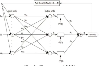
As applications of hybrid neural nets in this paper, we employ multipli-cation and addition to combine input signals and connection weights. 3.1. Input-output relations of each unit. Now consider a two-layer hybrid FNN with (N + 1) input units and (N + 1) output units such that all input-output signals and connection weights be real numbers. Suppose an input vector A= (A0, A1, ..., AN) is presented to our FNN,
then the input-output relation of each unit can be written as follows: Input units:
The input neurons make no change in their inputs, so: (3.1) oi =Ai, i= 0,2, ..., N.
Output units:
yj =f(netj),
netj =
N
X
i=0
wji.oi, j= 0,2, ..., N.
whereAi is a real number. In above equationwjidenotes the connection
weight from the i-th input unit to the j-th output unit and f(x) is identical activation function corresponding to output nodes (see Fig. 1).
Fig. 1. The proposed FNN
3.2. Cost function. Let us define the parameters Ai, wji and target
vector B = (B0, ..., BN) as following:
Ai = F(i)(0), wji=
Ti,j , j 6=i,
Ti,j−1 , j =i, Bj = −f
(j)(0), j, i= 0, ...., N.
Suppose that Y = (Y0, ..., YN) be the output vector corresponding to
the input vector A = (A0, ..., AN). Now we want to introduce how
to deduce the learning algorithm from the training set {A;B}. To do this, we defined a cost function between the jth output unit Yj and
corresponding target outputBj as follows:
(3.2) ej =
(Bj−Yj)2
In general, the cost function for the input-output pair{A;B}is obtained as:
(3.3) e=
N
X
j=0
ej.
3.3. Learning algorithm of the FNN. The present algorithm intends to acquire the minimum of the cost function in weight space using the method of gradient descent. The combination of the connection weights which minimizes the error function is considered to be a solution of the learning problem. Let real quantitiesAi (f or i= 0, ..., N) are initialized
at random values for input signals. We want to update the crisp param-eter Ai such thatAi =F(i)(0). At first we calculate the parameterswji,
Tji and Yj (f or j, i= 0, ..., N) by using of relations that were described
at the begining of this section. For crisp parameter Ai adjustment rule
can be written as follows:
(3.4) Ai(r+ 1) =Ai(r) + ∆Ai(r),
(3.5) ∆Ai(r) =−η. ∂e ∂Ai
+α.∆Ai(r−1), i= 0, ..., N,
where r is the number of adjustments, η is the learning rate and α is the momentum term constant. Thus our problem is to calculate the derivative ∂e
∂Ai in (3.5). The derivative ∂e
∂Ai can be calculated from the
cost function ein (3.3). We calculated ∂A∂e
i as follows:
(3.6) ∂e
∂Ai
= ∂e1
∂Ai
+· · ·+∂eN
∂Ai
, i= 0, ..., N.
On the other hand,
∂ej ∂Ai
= ∂ej
∂Yj
. ∂Yj
∂netj
. ∂netj
∂Ai
= (f(j)(0) +Yj). ∂netj
∂Ai
, j= 0, ..., N,
where
∂netj ∂Ai
=
Tij , j6=i,
T ij−1 , j=i.
Let us assume input-output pair {A;B} that is given as training data, is applied for learning of the FNN. Then the learning algorithm can be summarized as follows:
Learning algorithm
Ai (f or i= 0, ..., N) are initialized at random values.
Step 2: Let r := 0 wherer is the number of iterations of the learning algorithm. Then the running error E is set to 0.
Step 3: Letr :=r+ 1. Then,
i): Forward calculation: Calculate the output vector Y by pre-senting the input vector A.
ii): Back-propagation: Adjust crisp parameterAiusing the cost
function (3.3).
Step 4: Cumulative cycle error is computed by adding the present error to E.
Step 5: The training cycle is completed. ForE < Emax terminate the training session. If E > Emax thenE is set to 0 and we initiate a new training cycle by going back to Step 3.
4. Numerical examples
This section contains three examples of linear Fredholm integral equa-tions of second kind. In these examples, we illustrate the use of FNN technique to approximate the solutions of the given integral equations. For each example, the computed values of the approximate solution are calculated over a number of iterations and the cost function is plotted. Moreover the present method is compared with trapezoidal quadrature rule and a type of artificial neural networks that has been introduced in [2]. In the following simulations, we use the specifications as follows:
1. Learning constant η= 0.5. 2. Momentum constant α= 0.5. 3. Stoping conditions Emax <0.0001.
Example 1. Consider the following Fredholm integral equation
F(t) =sin(t)− 1 4t+
1 4
Z π2
0
tsF(s)ds,
with the exact solutionF(t) = sint. For this case, we used a polynomial of degree 7. We trained FNN with 8 input units and 8 output units. We choose an initial approximation polynomial of degree 7 for unknown functionF(t) as follows:
1. Learning constant η= 0.5. 2. Momentum constant α= 0.5. 3. Stoping conditions Emax <0.0001.
Example 1. Consider the following Fredholm integral equation
F(t) =sin(t)−1 4t+
1 4
Z π2
0
tsF(s)ds,
with the exact solution F(t) = sint. For this case, we used a polynomial of degree 7. We trained FNN with 8 input units and 8 output units. We choose an initial approximation polynomial of degree 7 for unknown function F(t) as follows:
F(t) = 1 2+
1 2t−
1 4t
2− 1
12t
3+ 1
48t
4+ 1
240t
5− 1
1440t
6− 1
10080t
7.
From above polynomial, initial input vector can be written as
A= (0.5,0.5,−0.5,−0.5,0.5,0.5,−0.5.−0.5).
After 14 iterations the approximate function F(t) transformed to fol-lowing form:
F(t) =−1.9841×10⁻⁴ t7+1.8701×10⁻⁸t6+0.0083 t5+9.0953×10⁻⁶ t4
−0.1666 t3+ 7.9622×10⁻⁴ t2+ 0.9986 t+ 0.0026.
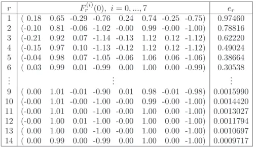
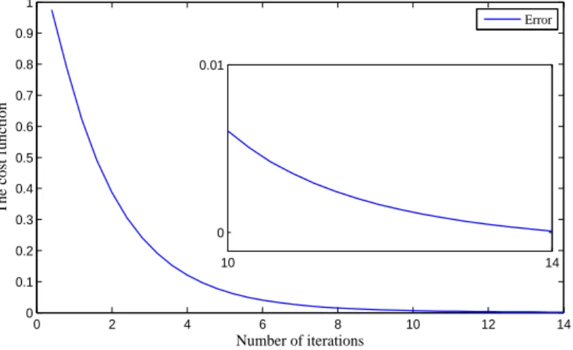
Table 1 shows the approximated solution over a number of iterations and Figs. 2 and 3 show the convergence behaviors for computed values of the parameter Fr(i)(0) for different numbers of iterations.
r Fr(i)(0), i= 0, ...,7 er
1 ( 0.18 0.65 -0.29 -0.76 0.24 0.74 -0.25 -0.75) 0.97460 2 (-0.10 0.81 -0.06 -1.02 -0.00 0.99 -0.00 -1.00) 0.78816 3 (-0.21 0.92 0.07 -1.14 -0.13 1.12 0.12 -1.12) 0.62220 4 (-0.15 0.97 0.10 -1.13 -0.12 1.12 0.12 -1.12) 0.49024 5 (-0.04 0.98 0.07 -1.05 -0.06 1.06 0.06 -1.06) 0.38664 6 ( 0.03 0.99 0.01 -0.99 0.00 1.00 0.00 -0.99) 0.30538
..
. ... ...
9 ( 0.00 1.01 -0.01 -0.90 0.01 0.98 -0.01 -0.98) 0.0015990 10 (-0.00 1.01 -0.00 -1.00 -0.00 0.99 -0.00 -1.00) 0.0014420 11 (-0.00 1.01 0.00 -1.00 -0.00 1.00 0.00 -1.00) 0.0013027 12 (-0.00 1.00 0.01 -1.00 -0.00 1.00 0.00 -1.00) 0.0011794 13 ( 0.00 1.00 0.00 -1.00 -0.00 1.00 0.00 -1.00) 0.0010697 14 ( 0.00 0.99 0.00 -0.99 0.00 1.00 0.00 -1.00) 0.0009717 Table 1. The approximated solutions with error analysis for Example 1.
0 2 4 6 8 10 12 14 0
0.1 0.2 0.3 0.4 0.5 0.6 0.7 0.8 0.9 1
Number of iterations
The cost function
Error
10 14
0 0.01
Fig. 2. The cost function for Example 1.
2 4 6 8 10 12 14 16
−1.5 −1 −0.5 0 0.5 1 1.5
Number of iterations
F(0) F’(0) F’’(0) F’’’(0) F(4)(0) F(5)(0) F(6)(0) F(7)(0)
Fig. 3. Convergence of the calculated solutions for Example 1.
Trapezoidal rule: Moreover, this example is going to show differ-ence between the FNN approach and the trapezoidal quadrature rule. Consider again Example 1, the trapezoidal quadrature procedure is as follows:
Let the region of integration is subdivided into 4 equal intervals of width
h = π8, 5 integration nodes ti = (i−81)π and fi =f(ti) (f or i= 1, ...,5).
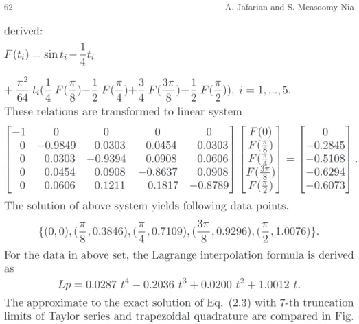
derived:
F(ti) = sinti−
1 4ti
+ π
2
64 ti( 1 4F(
π
8)+ 1 2F(
π
4)+ 3 4F(
3π
8 )+ 1 2 F(
π
2)), i= 1, ...,5. These relations are transformed to linear system
−1 0 0 0 0
0 −0.9849 0.0303 0.0454 0.0303 0 0.0303 −0.9394 0.0908 0.0606 0 0.0454 0.0908 −0.8637 0.0908 0 0.0606 0.1211 0.1817 −0.8789 F(0)
F(π8)
F(π4)
F(38π)
F(π2) = 0 −0.2845 −0.5108 −0.6294 −0.6073 .
The solution of above system yields following data points, {(0,0),(π
8,0.3846),(
π
4,0.7109),( 3π
8 ,0.9296),(
π
2,1.0076)}. For the data in above set, the Lagrange interpolation formula is derived as
Lp= 0.0287 t4−0.2036 t3+ 0.0200 t2+ 1.0012 t.
The approximate to the exact solution of Eq. (2.3) with 7-th truncation limits of Taylor series and trapezoidal quadrature are compared in Fig. 4 with the exact solution.
0 0.5 1 1.5
0 0.2 0.4 0.6 0.8 1 t 1.5 1.56 0.997 1.008 t Exact solution FNN Trap. rule
Fig. 4. Comparison the exact and approximated solutions for Example 1.
Also Table 2 illustrates the absolute values of the errors obtained here and the absolute errors of [2] for this example. As showing, difference between the exact solution and the computed solution is dispensable.
P resented method N eural network approach$[2]
t= − − − − − − − − − − −− − − − − − − − − − − −
50iterations 100iterations 50iterations 100iterations
0 4.08×10⁻⁵ 6.35×10⁻⁹ 2.11×10⁻⁵ 6.35×10⁻⁸ Π
8 4.16×10−
5
5.80×10⁻⁹ 2.03×10⁻⁵ 5.66×10⁻⁸ Π
4 4.23×10−
5
5.08×10⁻⁹ 1.89×10⁻⁵ 6.10×10⁻⁸ 3Π
8 4.41×10−
5
7.15×10⁻⁹ 2.08×10⁻⁵ 7.03×10⁻⁹ Π
2 4.68×10−
5
6.24×10⁻⁹ 2.05×10⁻⁵ 5.21×10⁻⁹
Table 2. Absolute errors with N = 8 for Example 1.
Example 2. Let us consider the integral equation
F(t) =et−e
t+1−1
t+ 1 +
Z 1 0
etsF(s)ds,
with the exact solutionF(t) =et. We trained the fuzzy neural network as described in last example. Before starting calculations, we assumed that F(i)(0) = 0.5,(f or i= 0, ..., N). Now we have:
F(t) = 1 2+
1 2t+
1 4t
2+ 1
12t
3+ 1
48t
4+ 1
240t
5.
After 30 iterations the approximate function F(t) transformed to the follow function:
F(t) = 0.0083 t5+ 0.0412 t4+ 0.1647 t3+ 0.4933 t2+ 0.9849 t+ 0.9736.
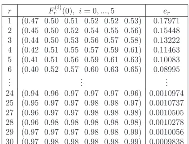
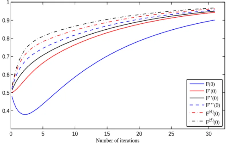
Numerical results can be found in Table 3. Similarly Figs. 5 and 6 show the accuracy of the solution or the convergence behaviors for computed values of the parametersFr(i)(0) where r is the number of iterations.
r Fr(i)(0), i= 0, ...,5 er
1 (0.47 0.50 0.51 0.52 0.52 0.53) 0.17971 2 (0.45 0.50 0.52 0.54 0.55 0.56) 0.15448 3 (0.44 0.50 0.53 0.56 0.57 0.58) 0.13222 4 (0.42 0.51 0.55 0.57 0.59 0.61) 0.11463 5 (0.41 0.51 0.56 0.59 0.61 0.63) 0.10083 6 (0.40 0.52 0.57 0.60 0.63 0.65) 0.08995
..
. ... ...
24 (0.94 0.96 0.97 0.97 0.97 0.96) 0.0010974 25 (0.95 0.97 0.97 0.98 0.98 0.97) 0.0010737 27 (0.96 0.97 0.97 0.98 0.98 0.98) 0.0010505 28 (0.96 0.98 0.98 0.98 0.98 0.98) 0.0010278 29 (0.97 0.97 0.97 0.98 0.98 0.99) 0.0010056 30 (0.97 0.98 0.98 0.98 0.98 0.99) 0.0009838
Table 3. The approximated solutions with error analysis for Example 2.
0 5 10 15 20 25 30
0 0.02 0.04 0.06 0.08 0.1 0.12 0.14 0.16 0.18
Number of iterations
The cost function
20 25
1.9 3x 10
−3
Error
0 5 10 15 20 25 30 0.4
0.5 0.6 0.7 0.8 0.9 1
Number of iterations
F(0) F’(0) F’’(0) F’’’(0) F(4)(0) F(5)(0)
Fig. 6. Convergence of the calculated solutions for Example 2.
Trapezoidal rule: For this example the trapezoidal rule with 5 inte-gration nodes can be written as follows:
F(ti) =eti−
eti+1−1 ti+ 1
+1
8(F(0)+2e
1 4tiF(1
4)+2e
1 2tiF(1
2)+2e
3 4tiF(3
4)+e
tiF
(1)),
where
ti=
i−1
4 , i= 1, ...,5.
The solution of the linear system which is caused from above relations, yields following data points:
{(0,0.9156),(0.25,1.1938),(0.5,1.5538),(0.75,2.0194),(1,2.6213)}.
Similarly, the lagrange interpolation formula is came from above inter-polation pairs as
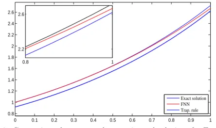
0 0.1 0.2 0.3 0.4 0.5 0.6 0.7 0.8 0.9 1 0.8
1 1.2 1.4 1.6 1.8 2 2.2 2.4 2.6
t
Exact solution FNN Trap. rule
0.8 1
2.2 2.6
Fig. 7. Comparison the exact and approximated solutions for Example 2.
In Fig. 7, the differences between 5-th truncation limit of the Taylor series and the TQR with exact solution are quite noticeable.
Similarly Table 4 illustrates the absolute values of the errors obtained here and the absolute errors of [2] for example 2.
P resented method N eural network approach [2]
t= − − − − − − − − − − −− − − − − − − − − − − −
50iterations 100iterations 50iterations 100iterations
0 4.08×10⁻⁴ 3.65×10⁻¹⁰ 6.85×10⁻⁵ 1.86×10⁻⁸ 1
4 8.20×10−
5
1.15×10⁻¹⁰ 4.52×10⁻⁵ 2.06×10⁻⁸ 1
2 3.17×10−
4
3.46×10⁻¹⁰ 4.41×10⁻⁵ 7.84×10⁻⁹ 3
4 3.37×10−
4
3.70×10⁻¹⁰ 5.30×10⁻⁵ 8.11×10⁻⁹
1 1.09×10⁻³ 8.05×10⁻⁹ 4.08×10⁻⁵ 8.86×10⁻⁹
Table 4. Absolute errors withN = 6 for Example 2.
From examples (1) and (2) we can conclude that to get the best approx-imating solution for unknown function, the truncation limit N must be chosen large enough.
Example 3. Consider the following integral equation problem
F(t) = 2t+ Z 1
0
with the exact solutionF(t) =−12t−8. Similarly, we applied proposed scheme for this problem. The learning started by
F(t) =t2−10t−10.
After 313 iterations, the approximate function F(t) is given by
F(t) =−4.1380×10⁻⁴ t2−11.9394 t−7.9675.
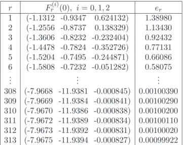
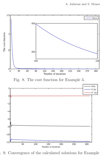
Numerical result can be found in tables 5 and 6. Figs. 8 and 9 show the convergence behaviors for computed values of the parameters Fr(i)(0),
where r is number of iterations. Moreover, exact solution and the ap-proximated solution are compared in Fig. 10.
r Fr(i)(0), i= 0,1,2 er
1 (-1.1312 -0.9347 0.624132) 1.38980 2 (-1.2556 -0.8737 0.138329) 1.13430 3 (-1.3606 -0.8232 -0.232404) 0.92432 4 (-1.4478 -0.7824 -0.352726) 0.77131 5 (-1.5204 -0.7495 -0.244871) 0.66086 6 (-1.5808 -0.7232 -0.051282) 0.58075
..
. ... ...
308 (-7.9668 -11.9381 -0.000845) 0.00100390 309 (-7.9669 -11.9384 -0.000841) 0.00100290 310 (-7.9670 -11.9386 -0.000838) 0.00100200 311 (-7.9672 -11.9389 -0.000834) 0.00100110 312 (-7.9673 -11.9392 -0.000831) 0.00100020 313 (-7.9675 -11.9394 -0.000827) 0.00099922
0 30 60 90 120 150 180 210 240 270 300 0
.5 1 1.5
Number of iterations
The cost function
150 210
001 002
Error
Fig. 8. The cost function for Example 3.
50 100 150 200 250 300
−12 −10 −8 −6 −4 −2 0 2
Number of iterations
F(0) F’(0) F’’(0)
Fig. 9. Convergence of the calculated solutions for Example 3.
Trapezoidal rule: Similarly, the trapezoidal rule with 5 integration nodes can be written as follows:
F(ti) = 2ti+
1
8(tiF(0)+2(ti+0.25)F( 1
4)+2(ti+0.5)F( 1
2)+2(ti+0.75)F( 3
4)+(ti+1)F(1)), where
ti=
i−1
The solution of the linear system which is caused from above relations, yields following data points:
{(0,−7.3333),(0.25,−10),(0.5,−12.6667),(0.75,−15.3333),(1,−18)}.
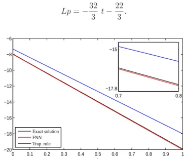
Similarly, by using the procedure which has been used for the previous examples, the Lagrange interpolation formula is derived as
Lp=−32
3 t− 22
3 .
0 0.1 0.2 0.3 0.4 0.5 0.6 0.7 0.8 0.9 1 −20
−18 −16 −14 −12 −10 −8 −6
t
0.7 0.8
−17.8 −15
Exact solution FNN Trap. rule
Fig. 10. Comparison the exact and approximated solutions for Example 3.
P resented method N eural network approach [2]
t= − − − − − − − − − − −− − − − − − − − − − − −
50iterations 100iterations 50iterations 100iterations
0 8.11×10⁻³ 7.06×10⁻⁵ 4.93×10⁻² 4.16×10⁻⁴ 1
4 2.01×10−
2
8.69×10⁻⁵ 3.81×10⁻² 2.59×10⁻⁴ 1
2 2.86×10−
2
1.90×10⁻⁴ 7.07×10⁻³ 6.72×10⁻⁵ 3
4 3.37×10−
2
3.04×10⁻⁴ 8.31×10⁻³ 3.62×10⁻⁴
1 3.70×10⁻² 3.73×10⁻⁴ 2.18×10⁻² 5.04×10⁻⁴
Table 6. Absolute errors with N = 4 for Example 3.
It is clear that using of this method we can find the analytical solution for these kinds of equations, if the exact solution of given problem be a polynomial.
5. Conclusions
In this paper, an architecture of feed-back neural networks has been proposed to approximate solution of a linear Fredholm integral equation of the second kind. Presented hybrid FNN in this study was a method for computing the coefficients in the Taylor expansion of unknown function. It is clear that to get the best approximate solution of the given equation, the truncation limit N must be chosen large enough. An interesting feature of this method is finding the analytical solution for the integral equation, if the exact solution of the problem be a polynomial of degree
N or less than N. Also, we have compared the purposed method with trapezoidal quadrature rule and, a structure of artificial neural networks which have been widely used to solve these kinds of equations. The analyzed examples illustrate the ability and reliability of the present method. The obtained solutions, in comparison with the exact solutions admit a remarkable accuracy. With the availability of this methodology, now it will be possible to investigate the approximate solution of other kinds of integral equations.
Acknowledgments
The authors are grateful to the anonymous referees for their comments which substantially improved the quality of this paper.
References
[1] S. Abbasbandy,Numerical solution of integral equation: Homotopy perturbation method and Adomians decomposition method, Appl. Math. Comput,173(2006), 493–500.
[2] S. Effati and R. Buzhabadi, A neural network approach for solving Fred-holm integral equations of the second kind, Neural Compt. Appl, (2010), doi: 10.1007/s00521-010-0489-y.339-355.
[3] M. El-Shahed, Application of Hes homotopy perturbation method to Volterras integro-differential equation, Int. J. Non. Sci. Num. Simul,6(2005),163–168. [4] A. Golbabai and B. Keramati, Modified homotopy perturbation method
for solving Fredholm integral equations, Chaos Soli. Frac, (2006), doi:10.1016/j.chaos.2006.10.037.
[5] M. Gulsu and M. Sezer,The approximate solution of high order linear difference equation with variable coefficients in terms of Taylor polynomials, Appl. Math. Comput,168(2005), 76–88.
[6] R. P. Kanwal and K. C. Liu,A Taylor expansion approach for solving integral equations, Int. J. Math. Educ. Sci. Technol,20(1989), 411–414.
[7] X. Lan,Variational iteration method for solving integral equations, Comp. Math. with Appl,54(2007), 1071–1078.
[8] S. J. Liao,Beyond perturbation: Introduction to the Homotopy analysis method, Chapman Hall/CRC Press, Boca Raton (2003).
[9] S. J. Liao,On the homotopy analysis method for nonlinear problems, Appl. Math. Comput,147(2004), 499–513.
[10] S. J. Liao, Notes on the Homotopy analysis method: some defini-tions and theorems, Commun. Nonlinear Sci. Numer. Simul, (2008) doi: 10.1016/j.cnsns.2008.04–013.
[11] S. J. Liao and Y. Tan,A general approach to obtain series solutions of nonlinear differential equations, Stud. Appl. math,119(2007), 297–355.
[12] K. Maleknejad and K. Nouri, Nosrati Sahlan M, Convergence of approximate solution of nonlinear FredholmHammerstein integral equations, Commun. Non-linear Sci. Numer. Simul,15(6)(2010), 1432–1443.
[13] K. Maleknejad and K. Nouri, Mollapourasl R, Existence of solutions for some nonlinear integral equations, Commun. Nonlinear Sci. Numer. Simul,14(2009), 2559–2564.
[14] K. Maleknejad, R. Mollapourasl and M. Alizadeh,Convergence analysis for nu-merical solution of Fredholm integral equation by Sinc approximation, Commun. Nonlinear Sci. Numer. Simul,16(2011), 2478–2485.
[15] S. Nas, S. Yalcynbas and M. Sezer, A Taylor polynomial approach for solving high-order linear Fredholm integrodifferential equations, Int. J. Math. Educ. Sci. Technol,31(2000), 213–225.
[16] N. Sezer,Taylor polynomial solution of Volterra integral equations, Int. J. Math. Educ. Sci. Technol,25(1994), 625–633.
[17] M. Sezer and M. Gulsu, A new polynomial approach for solving difference and Fredholm integro-difference equations with mixed argument, Appl. Math. Com-put,171(2004), 332–344.
[18] M. Sezer,A method for approximate solution of the second order linear differen-tial equations in terms of Taylor polynomials, Int. J. Math. Educ. Sci. Technol, 27(1996), 821–834.
Ahamad Jafarian
Department of Mathematics, Urmia Branch, Islamic Azad University, Urmia, Iran
Email: [email protected]
Safa Measoomy Nia
Department of Mathematics, Urmia Branch, Islamic Azad University, Urmia, Iran