Air-sea transfer of gas phase controlled compounds

(1)

This content has been downloaded from IOPscience. Please scroll down to see the full text.

Download details:

IP Address: 78.153.201.123

This content was downloaded on 06/06/2016 at 17:12

Please note that terms and conditions apply.

Air-sea transfer of gas phase controlled compounds

View the table of contents for this issue, or go to the journal homepage for more 2016 IOP Conf. Ser.: Earth Environ. Sci. 35 012011

(http://iopscience.iop.org/1755-1315/35/1/012011)

(2)

Air-sea transfer of gas phase controlled compounds

M Yang1_{, T G Bell}1_{, B W Blomquist}2_{, C W Fairall}2_{, I M Brooks}3_{and P D}

Nightingale1

1_{Plymouth Marine Laboratory, Prospect Place, Plymouth, UK}

2_{NOAA Earth System Research Laboratory, Boulder, Colorado, USA}

3_{Institute for Climate and Atmospheric Science, School of Earth and Environment,} University of Leeds, Leeds, UK

Email: miya@pml.ac.uk

Abstract. Gases in the atmosphere/ocean have solubility that spans several orders of magnitude. Resistance in the molecular sublayer on the waterside limits the air-sea exchange of sparingly soluble gases such as SF6 and CO2. In contrast, both aerodynamic and molecular diffusive

resistances on the airside limit the exchange of highly soluble gases (as well as heat). Here we present direct measurements of air-sea methanol and acetone transfer from two open cruises: the Atlantic Meridional Transect in 2012 and the High Wind Gas Exchange Study in 2013. The transfer of the highly soluble methanol is essentially completely airside controlled, while the less soluble acetone is subject to both airside and waterside resistances. Both compounds were measured concurrently using a proton-transfer-reaction mass spectrometer, with their fluxes quantified by the eddy covariance method. Up to a wind speed of 15 m s–1_{, observed air-sea}

transfer velocities of these two gases are largely consistent with the expected near linear wind speed dependence. Measured acetone transfer velocity is ~30% lower than that of methanol, which is primarily due to the lower solubility of acetone. From this difference we estimate the “zero bubble” waterside transfer velocity, which agrees fairly well with interfacial gas transfer velocities predicted by the COARE model. At wind speeds above 15 m s–1_{, the transfer velocities}

of both compounds are lower than expected in the mean. Air-sea transfer of sensible heat (also airside controlled) also appears to be reduced at wind speeds over 20 m s–1_{. During these}

conditions, large waves and abundant whitecaps generate large amounts of sea spray, which is predicted to alter heat transfer and could also affect the air-sea exchange of soluble trace gases. We make an order of magnitude estimate for the impacts of sea spray on air-sea methanol transfer.

1. Introduction

Many gases that exchange between the ocean and atmosphere influence our climate and air quality. In addition to carbon dioxide (CO2) and dimethylsulfide (DMS), the oceans can be a net source or sink of very soluble organic compounds such as methanol and acetone [1], which affect the atmosphere’s ability to cleanse itself of pollutants. Other soluble/reactive gases that cross the air/sea interface include sulfur dioxide (SO2 [2]), polychlorinated biphenyls (PCBs [3]), ozone [4], and oxygenated volatile organic compounds such as formaldehyde [5], acetaldehyde [6] and glyoxal [7].

Wind blowing over the ocean provides the predominant kinetic forcing for air-sea transfer, while the thermodynamic potential for exchange is governed by the air-sea gas disequilibrium. Based on the

two-7th International Symposium on Gas Transfer at Water Surfaces IOP Publishing IOP Conf. Series: Earth and Environmental Science 35 (2016) 012011 doi:10.1088/1755-1315/35/1/012011

(3)

layer model [2], the net air-sea gas flux is usually estimated from the gas transfer velocity (K) and the air-sea concentration gradient (∆C), with a positive flux indicating sea-to-air emission:

Flux = Ka (Cw/H – Ca) = Kw (Cw – HCa) (1)

The total gas transfer velocity from the air perspective (Ka) and water perspective (Kw) are related: Ka =

HKw, where H is the dimensionless liquid to gas solubility. Cw and Ca are the gas concentrations in water and air. Partitioning of ∆C and resistance to transfer in the two phases depend primarily on H:

Ka = 1/(1/ka + 1/(Hkw)) (2a)

Kw = 1/(1/kw + H/ka) (2b)

Here ka and kw are the individual transfer velocities in the gas phase and water phase, respectively.

Exchange of sparingly soluble gases (low H) is limited by the rate of transport in water (i.e., Kw≈kw),

while the exchange of highly soluble gases (high H) is limited by transport in air (i.e., Ka≈ka). CO2 and DMS are examples of sparingly soluble (waterside controlled) gases. The transfer of DMS is thought to be a mostly interfacial process and not very sensitive to bubbles [8, 9]. CO2 is less soluble than DMS so is subject to greater bubble-mediated exchange in addition to interfacial exchange [8]. The transfer of methanol, a gas ~500 times more soluble than DMS, is almost entirely controlled on the airside. Acetone, ~60 times more soluble than DMS, is subject to resistance both on the airside and on the waterside (~75% and 25% at 20ºC, respectively).

Current understanding of airside-controlled gas transfer stems mostly from measurements of water vapor (H2O, i.e., latent heat) and sensible heat. Similar to highly soluble gases, there is effectively no waterside resistance to heat transfer. Due in part to the much higher molecular diffusivities of gases in air than in water, turbulent resistance is relatively more important for ka (i.e., aerodynamic resistance)

than for kw. At moderate wind speeds, the transfer velocities of heat demonstrate a near-linear relationship to wind speed and to the friction velocity (u*). This results in fairly constant values of the dimensionless transfer coefficients for sensible heat, latent heat, and enthalpy (= sensible heat + latent heat) at around 1e–3_{[10]. At wind speeds over 20 m s}–1_{, limited heat transfer measurements demonstrate} a large range [11, 12]. In such high seas, model results suggest that sea spray from wave breaking plays an important role in heat transfer [13, 14]. Sea spray could also have an effect on the transfer of airside controlled compounds (analogous to the effect of bubbles upon kw). For example, sea spray has been

shown to be a source of atmospheric hydrochloric acid [15] and is thought to be a possible sink for atmospheric SO2 [16].

Direct air-sea transfer measurements of airside controlled trace gases (i.e., not H2O) are rare. Aircraft observations of the surface reactive SO2 yielded an airside transfer velocity that is ~30% lower than predicted [17], illustrating an uncertainty in our understanding of ka. Yang et al. (2013a) developed a

novel system to measure the air-sea transfer of methanol and acetone by eddy covariance using a proton transfer reaction mass spectrometer, PTR-MS [18]. Air-sea fluxes of these compounds were quantified during the Atlantic Meridional Transect cruise (AMT-22; [1, 19]) and more recently during the High Wind Gas Exchange Study (HiWinGS; [20]). Here we present a more in-depth analysis of the HiWinGS dataset, compare results from HiWinGS to those from AMT-22, and examine the potential effects of sea spray on methanol transfer.

2. Experimental

The transfer velocity of methanol (as well as sensible heat) was determined during the AMT-22 and the HiWinGS cruises. Acetone was measured with enough precision to derive its transfer velocity only on the HiWinGS cruise. The experimental settings and methods have been described in detail previously [1, 19, 20]. Very briefly, concentrations of both compounds in the atmosphere and surface ocean were quantified by a PTR-MS. For the majority of the cruise, the PTR-MS was operated in atmospheric mode and sampling at a rate just above 2 Hz. Winds and motion were measured by a sonic anemometer (Gill

7th International Symposium on Gas Transfer at Water Surfaces IOP Publishing IOP Conf. Series: Earth and Environmental Science 35 (2016) 012011 doi:10.1088/1755-1315/35/1/012011

(4)

Windmaster) and Motionpak (Systron Donner) co-located with the gas inlet on the foremast of the ship. Wind velocities corrected for ship’s motion ([21] followed by sequential decorrelations with the ship’s motion) were used to compute the fluxes of methanol, acetone, sensible heat, and momentum by the eddy covariance method. Approximately twice a day, the PTR-MS was switched to analyze discrete water samples for dissolved concentrations of methanol and acetone [22]. Near-surface waters were taken at a few meters below the ocean surface from twice-a-day CTD casts as well as from the ship’s non-toxic underway water supply. The total transfer velocities of methanol and acetone from the atmospheric perspective were computed by dividing the measured fluxes by the air-sea concentration difference following equation 1.

HiWinGS methanol and acetone data presented in this paper have been reprocessed since Yang et al. [20]. The major differences in this processing are 1) compute fluxes as 20-minute averages instead of hourly averages. The 20-minute averages are then binned into hourly intervals (hours with less than two valid intervals are not considered for further analysis). Signal dropout and elevated noise at high frequencies were common for the Windmaster sonic anemometer during moderate-to-heavy precipitation, which tended to coincide with very high wind speeds. The shorter averaging time afforded ~15% more useable flux data that were previously discarded due to episodic rain events; 2) correct the

w axis of the Windmaster sonic anemometer for a calibration bias. On the advice of the manufacturer Gill (R. McKay, personal communication, 2015), we applied a bias correction to the raw w data of the Windmaster (+16.6% for positive w; 28.9% for negative w). The same w correction has also been applied to the AMT-22 dataset.

3. Results and discussion

3.1. Reprocessed HiWinGS results

The mean cospectra of methanol, acetone, and sonic heat flux for the HiWinGS cruise are shown in

figure 1. Heat flux was upwards, while both methanol and acetone fluxes were downwards. The cospectra of the two gases show comparable flux magnitudes and are fairly similar in shape to that of the sonic heat flux. Due to the relatively low sampling rate of the PTR-MS, flux attenuation is evident for the gases at high frequencies, which was corrected using a filter function approach [18, 20]. For this cruise, averaging to 20 minutes instead of an hour also results in a very small loss (~1%) in the gas fluxes at low frequencies.

Compared to [20], the reprocessed methanol and acetone fluxes (as well as transfer velocities) are ~15% higher in the mean, as expected from the Gill bias correction. This correction also increases u*

by ~5%, which remains close to the predicted value from COARE 3.5 [23]. The hourly methanol and

Figure 1. Mean cospectra of the oxygenated volatile organic compounds (OVOCs) methanol, acetone, and sonic heat flux during HiWinGS.

(5)

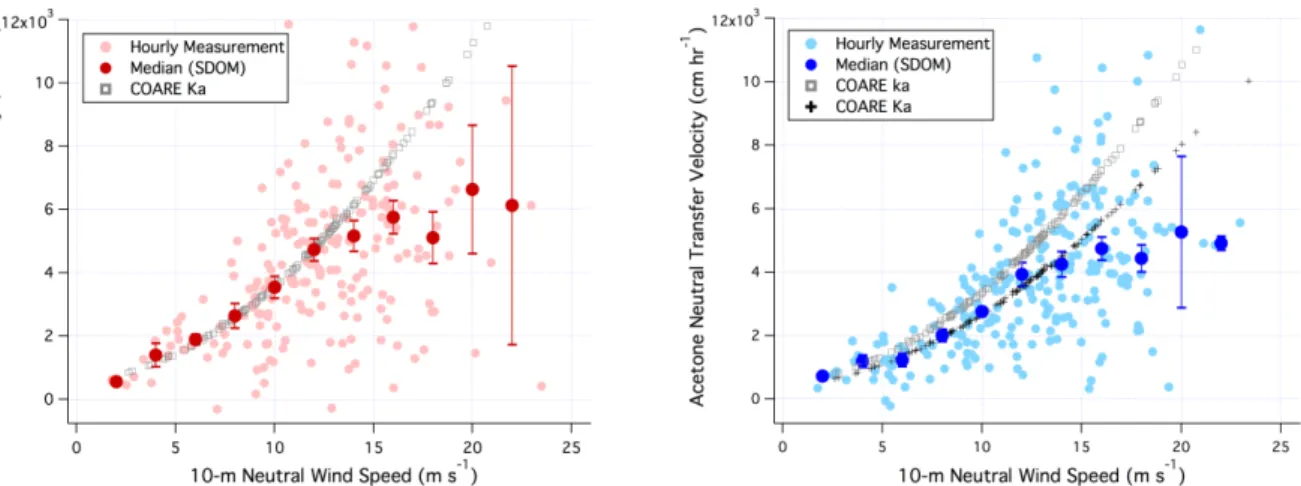
acetone transfer velocities (KMETHANOL and KACETONE) are plotted against 10-m neutral wind speed (U10n)

in figure 2, along with bin-medians and standard errors. They have been adjusted to a neutral atmosphere using the stability parameter from the COARE bulk output (e.g., [24]). We also plot the COARE [10] total gas transfer velocity from the atmospheric perspective (Ka) for methanol and acetone, as well as

the airside transfer velocity (ka) for acetone (note that Ka≈ka for methanol). At wind speeds less than 15 m s–1_{, there is close agreement between measured and predicted}_Ka_{for methanol as well as for} acetone. Both show a slight non-linear dependence on wind speed (and increase essentially linearly with

u*). Between 15 and 20 m s–1, measured KMETHANOL and KACETONE are lower than the model predictions,

with the more soluble methanol showing a greater discrepancy. The measurement–model bias increases with wind speed. For example, the respective measurement/model ratio for KMETHANOL is 0.74 and 0.55

at wind speeds of 16 and 18 m s–1_{. For acetone, this ratio is 0.84 and 0.66, respectively. These results} suggest a possible suppression of gas transfer that is primarily on the airside.

Gas transfer velocity data at wind speed over 20 m s–1_{are still very limited (only six valid hours),} resulting in highly uncertain bin medians. This is partly because the air-sea ∆C of these gases is dominated by their atmospheric abundance, which tended to be low in storms as a result of precipitation scavenging [20]. To reduce noise in Ka, we have neglected periods when the atmospheric mixing ratio

is below 0.2 ppb. Air-to-sea (dry) deposition removes these gases from the marine atmospheric boundary layer at a timescale of 1–2 days [20]. Due to its higher solubility, wet deposition is more important of a sink for atmospheric methanol than for acetone [20]. Both of these gases have large terrestrial sources. Measuring in a region of higher atmospheric organic abundance (e.g., downwind of a continent) could help to reduce the uncertainties in KMETHANOL and KACETONE.

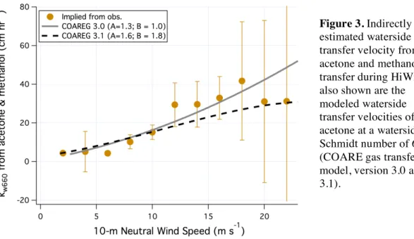
As mentioned previously, acetone transfer is subject to significant resistance on both the air side and on the water side. From the bin-medians of KACETONE and KMETHANOL, we rearrange equation 2a and compute the waterside transfer velocity kw = 1/(H(1/Ka – 1/ka)). This analysis was done previously [20] but only at a single wind speed of 12 m s–1_{(HiWinGS mean). Here we illustrate the wind speed} dependence in waterside transfer (figure 3). For this calculation we assume KMETHANOL = ka of acetone.

We further normalize kw to a Schmidt number of 660, e.g., kw660 = kw * (ScACETONE/660)1/2_{, where}_ScACETONE is the ambient Schmidt number of acetone. The resultant kw660 should represent a “zero-bubble” (i.e., purely interfacial) waterside transfer velocity. Also shown in figure 3 are the predicted waterside transfers from the COARE gas transfer model version 3.0 (empirical constants A = 1.3 for interfacial transfer and B = 1.0 for bubble-mediated transfer) and version 3.1 (A = 1.6, B = 1.8, tangential u* instead

of total u*) [10]. The constant B is essentially irrelevant here because bubble-mediated exchange for the

very soluble acetone is effectively zero. Both versions of the COARE model fit through the HiWinGS results. Due to the large uncertainties in kw660 (propagated from the standard errors shown in figure 2),

especially in high winds, neither version of the model performs better/worse than the other compared to

Figure 2. Methanol transfer velocity (left) and acetone transfer velocity (right) from HiWinGS.

(6)

observations. Uncertainties in this indirect estimation of kw660 could be reduced by measuring acetone

in warm waters, as water side resistance becomes more important with increasing temperature.

3.2. Comparison between HiWinGS and AMT-22

We compare HiWinGS and AMT-22 in methanol and sensible heat transfer. To reduce noise in the methanol measurement, here we compute KMETHANOL as flux averaged over 8 hours divided by ∆C

averaged over 8 hours. As in [19], for this calculation the seawater methanol concentration is set to zero for the AMT-22 cruise. At a wind speed below 15 m s–1_,_K

METHANOL from the two cruises demonstrate

similar trends on average. The mean (±1 standard deviation) dimensionless methanol transfer coefficient (KMETHANOL /U10n) is 0.98 ± 0.39 e–3 from AMT-22 and 1.09 ± 0.35 e–3 from HiWinGS.

The AMT-22 cruise only had a few hours with wind speeds over 15 m s–1_{, during which}_K

METHANOL

appeared to be greater than the COARE prediction. This was initially interpreted to be due to an overestimation of the airside diffusive resistance in the COARE 3.0 model (and thus underestimation of the airside transfer velocity) [19]. The COARE model version 3.5 has a higher drag coefficient (i.e., lower aerodynamic resistance) than COARE 3.0 at high wind speeds. Implementing the COARE 3.5 drag coefficient (CD) into the gas transfer model would also result in a slightly higher ka to wind speed relationship than predicted using COARE 3.0. As shown in figure 4, these two model parameterizations start to diverge at a wind speed of ~15 m s–1_{. Considering methanol observations from both cruises (with} HiWinGS making up the bulk of the data at wind speeds over 10 m s–1_{), both versions of the model} appear to fit observations fairly well up to ~16 m s–1_.

Sensible heat transfer velocity (KHEAT) was computed from the sonic heat flux (corrected for humidity

using the bulk latent heat flux) and the air-sea potential temperature difference, and was further adjusted to a neutral atmosphere. As with methanol, below 15 m s–1_{there is fairly good agreement in}_K

HEAT

between the two cruises. Three parameterizations of KHEAT are shown. Two are derived from airside

resistance using CD from COARE 3.0 and 3.5. The other is a product of CHn and U10n, where the sensible

heat transfer coefficient CHn is an empirical fit to previous open ocean transfer measurements. These

parameterizations began to diverge above a wind speed of ~15 m s–1_{, with the empirical fit noticeably} lower than the resistance-based estimates. Due to the large scatter in measured KHEAT at wind speeds

above 15 m s–1_{, we are unable to discern which parameterization is the most appropriate. Interestingly,}

Figure 3. Indirectly estimated waterside transfer velocity from acetone and methanol transfer during HiWinGS; also shown are the modeled waterside transfer velocities of acetone at a waterside Schmidt number of 660 (COARE gas transfer model, version 3.0 and 3.1).

(7)

above a wind speed of ~20 m s–1_{, limited}_K

HEAT measurements appear to be lower than expected from the

COARE model. This is primarily because the measured sensible heat flux was ~40 W m–2_{lower than} predicted during the storm around 25 October 2013. We note that a low sensible heat transfer rate between 18 and 20 m s–1_{has been observed in a previous study [10]. Makin (1998) also modeled a} reduction in the sensible heat transfer coefficient and an increase in the latent heat transfer coefficient due to spray, which becomes important at wind speeds over 25 m s–1_{[14]. Below we crudely examine} the effects of spray on methanol transfer.

3.3. Impact of sea spray on methanol transfer

Sea spray lofted into the atmosphere is rapidly equilibrated in temperature with the surrounding air [13, 25]. When the sea surface is warmer than the air above, this leads to an initial warming of the near surface air. Partial evaporation of spray droplets gives off water vapor and cools the spray-evaporation layer (approximately equivalent to the significant wave height) over a longer timescale [25]. A net cooling in the spray-evaporation layer should reduce the vertical temperature gradient between the lowest meters of the atmosphere and the sonic anemometer (nominally ~20 m above sea level). This in

Figure 4. Transfer velocity of methanol from AMT-22 and HiWinGS cruises.

Figure 5. Transfer velocity of sensible heat from AMT-22 and HiWinGS cruises.

(8)

theory may lead to a covariance sensible heat flux at 20 m that is lower than predicted from bulk air/water temperatures. Some methanol is likely co-emitted during spray evaporation, which could possibly reduce the vertical methanol gradient between the lowest meters of the atmosphere and the gas inlet. However, there is the competing effect of spray absorption. Droplets initially undersaturated in methanol could take up the gas from the atmosphere and enhance air-to-sea methanol deposition.

Andreas et al. (1995) predicted that at a wind speed of 20 m s–1_{, the sea spray contribution to latent} heat flux and sensible heat is 150 and 15 W m–2_{, respectively [13]. The latter is of the same order of} magnitude (but opposite sign) to the discrepancy of ~40 W m–2_{in sensible heat flux (section 3.2).} Dividing by the density of air and latent heat of evaporation, 150 W m–2_{of latent heat from spray can be} converted to 0.05 g of water/kg of air • m s–1_{, or 0.06 g m}–2_s–1_{. Assuming spray initially carries the} same dissolved methanol concentration as seawater during HiWinGS (~20 nmole L–1_{), 0.06 g of water} would contain 1.2 pmole of methanol. This implies a spray-mediated methanol emission of 1.2 pmole m–2_s–1_{(if methanol is evaporated at the same rate as H2O) or ~0.1 µmole m}–2_d–1_{, which is on the order} of 1% of the measured methanol flux. It would take ~1 day for spray-mediated methanol emission to replace methanol within the lowest 5 m of the atmosphere – a timescale much longer than the eddy covariance averaging period.

We also consider the competing case of spray removing methanol from the atmosphere. The upper limit effect of this can be demonstrated by assuming all spray droplets reach methanol saturation (from an initial concentration of zero) with the atmosphere before falling back to the ocean. At a wind speed of 20 m s–1_{, the total mass concentration of sea spray is on the order of 1 g of spray/m}3_{of air [26]. During} HiWinGS, the equilibrium methanol concentration with the atmosphere (HCa) is on the order of 100

µmole/m3_{of water. Thus 1 g of spray/m}3_{of air can take up a maximum of 0.1 nmole of methanol/m}3_of air. This is two orders of magnitude lower than the actual atmospheric methanol concentration. From these calculations, droplet capacity appears to be a limitation to any spray-mediated methanol transfer. The seawater concentration as well as solubility of acetone are lower than those of methanol and we expect the effect of spray on acetone to be even less.

Key uncertainties in the estimations above include the spray source function and the size distribution of the spray droplets. Clearly, further measurements in high winds are needed to more accurately constrain the effect of sea spray on airside gas transfer.

4. Conclusions

In this contribution, we first presented reprocessed methanol and acetone transfer velocities from the HiWinGS cruise. Both transfer rates are close to COARE predictions at wind speeds less than 15 m s–1_. At higher wind speeds, measured methanol and acetone transfer velocities appear to be lower than predicted, with the more soluble methanol showing a greater deviation. From the difference between methanol and acetone transfer, we estimated the waterside “zero bubble” transfer velocity, which is fairly close to the COARE predictions for interfacial transfer. We compared the AMT-22 and the HiWinGS cruise in methanol and sensible heat transfer. At wind speeds below 15 m s–1_{, measurements} from the two cruises demonstrate good agreement for both scalars. Above 20 m s–1_{, measured sensible} heat transfer during HiWinGS is lower than the model prediction, qualitatively similar to the behavior of methanol. We crudely estimated the order of magnitude effect of sea spray on methanol transfer, which appears to be small. The reasons for the low gas and sensible heat transfer rates at high wind speeds during HiWinGS remain to be explained.

References

[1] Yang M et al 2014 Atmos. Chem. Phys. 14 7499 [2] Liss P S and Slater P G 1974 Nature247 181 [3] Jurado E et al 2004 Environ. Sci. Technol.38 5505 [4] Lenschow D H et al 1981 J. Geophys. Res. 86 7291 [5] Zafiriou O C et al 1980 Geophys. Res. Lett.7 341

[6] Beale R et al 2013 J. Geophys. Res. 118 doi:10.1002/jgrc.20322

(9)

[7] Coburn S et al 2014 Atmos. Meas. Tech.7 3579

[8] Blomquist B et al 2006 Geophys. Res. Lett. 33 doi:10.1029/2006GL025735 [9] Yang M et al 2011 J. Geophys. Res. 116 doi:10.1029/2010JC006526 [10] Fairall C W et al 2011 J. Geophys. Res. 116 doi:10.1029/2010JC006884 [11] Bell M M et al 2012 J. Atmos. Sci., 69 3197

[12] Zhang J A et al 2008 Geophys. Res. Lett.35 doi:10.1029/2008GL034374 [13] Andreas E L et al 1995 Bound.-Layer Meteor. 72 3

[14] Makin V K 1998 J. Geophys. Res. 103 1137 [15] McInnes L M et al 1994 J. Geophys. Res. 99 8257 [16] Sievering H et al 1991 Atmos. Environ.25A 1479 [17] Faloona I et al 2010 J. Atmos. Chem. 63 13 [18] Yang M et al 2013 Atmos. Chem. Phys. 13 6165

[19] Yang M et al 2013 Proc. Natl. Acad. Sci. 110 doi:10.1073/pnas.1317840110 [20] Yang M et al 2014 J. Geophys. Res. Oceans119 doi:10.1002/2014JC010227 [21] Edson J et al 1998 J. Atmos. Oceanic Technol. 15 547

[22] Beale R et al 2011 Analytica Chimica Acta706 128 [23] Edson J B et al 2013 J. Phys. Oceanogr. 43 1589 [24] Fairall C W et al 1996 J. Geophys. Res. 101 3747 [25] Andreas E L 2010 J. Phys. Oceanogr. 40 608

[26] Fairall C W et al 2009 J. Geophys. Res. 114 doi:10.1029/2008JC004918