Finite Element Model for Linear Second Order One Dimensional Inhomogeneous Wave Equation

Finite Element Model for Linear Second Order One Dimensional

Inhomogeneous Wave Equation

Zain Ulabadin Zafar*1, A. Pervaiz2, M.O. Ahmed 2 and M. Rafiq1

1. Faculty of Information Technology, University of Central Punjab, Lahore, Pakistan 2. Department of Mathematics, University of Engineering & Technology, Lahore, Pakistan * Corresponding Author: e-mail: [email protected]

Abstract

In physics, propagation of sound, light and water waves is modeled by hyperbolic partial differential equations. Linear second order hyperbolic partial differential equations describe various phenomena in acoustics, electromagnetic and fluid dynamics. In this paper, a Galerkin based Finite Element Model has been developed to solve linear second order one dimensional Inhomogeneous wave equation numerically. Accuracy of the developed scheme has been analyzed by comparing the numerical solution with exact solution.

Key Words

: Finite Element Model, Galerkin Method, Lagrangian polynomials, Shape functions.

1. Introduction

Partial Differential Equations (PDE’s) are at the heart of many, if not most, computer analysis or simulations of continuous physical systems, such as fluids, electromagnetic fields, and the human body and so on [1]. A class of hyperbolic Partial Differential Equations which describes vibrations with in objects and how waves are propagated is called wave equation [2]. In physics, propagation of sound, light and water waves is modeled by hyperbolic partial differential equations. Linear second order hyperbolic partial differential equations

describe various phenomena in acoustics,

electromagnetic and fluid dynamics. The efficient and accurate numerical techniques for the wave equations is of fundamental importance for the

simulation of time dependent acoustic,

electromagnetic or elastic wave phenomena [3]. Finite difference methods are commonly used for the simulations of time dependent waves because of their simplicity and their efficiency on structured Cartesian meshes [4-6]. However in presence of complex geometry, their usefulness is somewhat limited. In contrast Finite Element Methods [7, 8] can easily handle these cases. Moreover their extension to higher order is straightforward. In this paper, a Finite Element Model for linear second order one dimensional inhomogeneous wave equation has been developed. Galerkin method has been used to setup

the element equations and a central finite difference scheme has been used to approximate the second order time derivative. Accuracy of the developed Finite Element model has been analyzed by comparing the computed solution with exact solution.

2. Finite Element Model

Consider the second order one dimensional Inhomogeneous Wave equation

l x x

x f t

f _{  }

    

0 ,

sin

2 2 2 2



 (1)

with boundary conditions

0 ,

0 ) , ( ) , 0

( t f l t  t

f

and initial conditions

l x xt

x

f( ,0)( ), 0  and

l x x

x t

f _{  }

 

0 ), ( ) 0 ,

( 

2.1 Domain Discretization

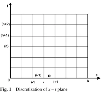
Let us consider the global domain as shown in figure1 in which we have to approximate the solution of equation (1). We divide the global domain into finite number of rectangular elements. Let there be K

nodes and K-1 linear elements in spatial direction. In the figure1, i represents ith node and (i) represents the ithelement. Each element has two nodese. g. element (i) has left node i and right node i1. The length of element (i) is given by x_i x_i1x_i. In a similar way we take an element along temporal axis each of length tn tn1tn,

Fig. 1 Discretization of x – t plane 2.2 Interpolating Functions

Let us approximate the solution of equation (1) by f(x,t), where f(x,t) is defined as

) , ( ... ) , ( ) ,

(xt f(1) xt f(1) xt

f   

) , ( ...f(K1) xt

 (2)

where each f(1)(x,t) (i1,2,3,...K1) represents the local interpolating polynomials over the element

) (i .

Write f(1)(x,t) for ith element as ) ( ) ( ) ( ) ( ) ,

( () ₁ ()₁

) 1

( _{xt f t N x f t N x}

f  _{i i}i  _{i i}i

(3)

Where f_i(t)(i1,2,...K) represents the nodal values and N_i(i) and N_i(i1) represent the shape functions for the element (i) at nodes i and i1 respectively and N_is are Lagrangian polynomials of degree one. We define

i i i

i i i

i

x

x

x

x

x

x

x

x

N

















 1

1 1 )

(

)

(

(4)

and

i i i i

i i

i _x

x x x x

x x x N

     

 

1 )

(

1( ) ₍₅₎

Substituting the values from equations (4) and (5) into equation (3), we have

   

 

      

 

  

  _

i i i

i i i

i

x x x f x x x f t x

f()( , ) 1 ₁ (6)

2.3 Element Equations

In this section we apply Galerken method to approximate the solution of one dimensional wave equation given by eq.(1) i.e.,

x x

f t

f

sin

2 2 2 2



 

    

Whose residual is

x x

f t

f t x

R( , ) sin

2 2 2 2



 

    

 (7)

Let us define the integral l



f(x,t)



of weighted residual, which is developed by multiplying R(x,t) by weighting functions W_k(x)(k1,2,3,...) and integrating that integral over the entire domain. Then set this integral equal to zero. We take the general weighting function W(x). Therefore



( , )



₂ sin 0

2 2 2 0

     

  

     





x dx

x f t

f W t x f

l  









  

 







dx

x f aW dx

t f W t

x f

l b

a b

a 2

2 2

2

) , (

0

sin 



bW xdx

a 

(8)

Now solving the second integral in (8) by parts That is

dx x f x W x

f W dx x

f

aW b

a b

a b

a 

       

    





 

2 2

(9)

The factor

x f  

in first term on R.H.S., of equation (9) cancels out at all interior points when we

assemble the element equations. It exists only at first and last node when there are boundary conditions on derivatives. Therefore we will drop this term so that equation (8) will take the form





       







dx

x f x W dx t f W t x f l b a b

a 2 

2 ) , ( dx x W b a sin



(10)

Now the weighted residual integral l



f(x,t)



for the entire domain is expressed as sum of weighted residual integrals of each element (i)(i1,2,...K).



f(x,t)



l()



f(x,t)



...l()



f(x,t)



...

l i i



( , )



0

) 1

(  _{f xt }

l K (11)

where





       









 dx

x f x W dx t f W t x f l i i i i x x i x x

i 1 1

2 ) ( 2 ) ( _{( , ) } dx x W i i x x sin 1 



 (12)

To evaluate l(i)



f(x,t)



given by equation (12). We require f(i)(x,t) and its partial derivatives w.r.t., t and.

Differentiating (3) two times partially w.r.t., ‘t’and substituting values of N_is from (4) and (5) we get                           i i i i i l i x x x f x x x f t f 1 1 2 ) ( 2 (13)

Now differentiating w.r.t

                    i i i i i x f x f x

f 1 1

1 ) ( ) ( 1 1 ) ( i i i i f f x x f       (14)

Substituting the values from equations (13) and (14) into equation (12)





             



  i i i x x i x x x f W t x f l i i 1 ) ( 1 ) , (



                         _

1 1 1

i i x x _i i i i i i dx x f f x W dx x x x f 



1 ₍₎

sin i i x x i _dx x

W (15)

Writing equation symbolically as



f xt



A B C

l(i) ( , )    (16)

Where A, B and C represents the integrals in equation (15). In Galerkin method, the weighted functions W_k(k1,2,...) are considered to be shape functions. Here N_i(i)(x) and N_i(_i)₁(x) are the shape function. Therefore let

i i i i _x x x x N x W    

 ()_{( )} 1

)

( and

i x x W    _ 1

Substituting the value of W(x) and _W_x in equation (15) and solving the integrals for A, B and C

dx f f A i i i i i i i i x x x i x x x i x x x x x     _                



 _  _  _{ } 1 1 1 ₁ ] 2 [

6  1



 xi _{fi fi}

A (17)

Next solving for B

dx x f f x B i i i i x x i i                





1 1 1

 ] [ ₁ 1 i i i x

x x f f

B i

i

 





  _ (18)

Solving for the value of C

dx x W

C x i

x i i ) ( sin 1 



  



()



sin 2 ) ( _i ave i x x

C     (19)

Where x_ave(i) is average values of x_i and x_i1

equations (17), (18) and (19) in equation (16) we have







 







    

 _{ i i}

i i

i i

i _{f f}

x f

f x t x f

l() 2 _{1 1}

6 ) ,

( 



sin



0 2

)

( (i) _

ave

i _x

x



(20)

Further we let, W(x)N_i(_i)₁(x), then

i i x

x x x W

  

)

( and

i x x W

  

 1

Next we use these values of W(x) and

x W  

equation (15), and solving for A, B, C we get.

dx x

x x f x x x f x

x x A

i i i

i i i

i i x

x

i

i 

   

  

   

 

       

 

        

 





1 1 _1



2 1



6  



 xi _{fi fi}

A (21)

Now

dx x

f x x B

i i i i x

x

i i

   

 

  

     





1_ 1 1



i i



i

f f x

B 



  _1 (22)

Solving for C we have



x



dx x

x x

C _avei

i i x

x

i i

) (

sin

1

     

  





 



()



sin 2

)

( i

ave i

x x

C    (23)

Now substituting values from equations (21), (22) and (23) into equation (16), we have:

















  



 _{ i i}

i i

i i

i _{f f}

x f

f x t x f

l() 2 _{1 1}

6 ) ,

( 



sin



0 6

)

( (i) _

ave

i _x

x



(24) equations (21) and (26) are the element equations for

ith element.

2.4 Assembly of Element Equations

Since ith node is common between (i) and )

1

(i element therefore in order to get the nodal

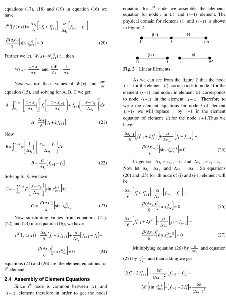
equation for ith node we assemble the elements equation for node i in (i) and (i1) element. The physical domain for element )(i and (i1) is shown in Figure 2.

Fig. 2 Linear Elements

As we can see from the figure 2 that the node 1



i for the element )(i corresponds to node i for the element (i1) and node i in element )(i corresponds to node (i1) in the element (i1). Therefore to write the element equations for node i of element

) 1

(i we will replace i by i1 in the element equation of element (i)for the node i1.Thus we have:













     

 

 

1 1

1

1 ₂

6 i i _i i i

i _{f f}

x f f

x 



sin



0 6

)

( 1 (i1) _

ave

i _x

x



(25) In general x_ix_i1x_i and x_i1x_ix_i1. Now let x_i x_ and xi_1x_. So equations

(20) and (25) for ith node of (i) and (i-1) element will be













     

   

i i i

i f f

x f

f x

1 1

6





sin



0 6

)

(  (i) _

ave x x



(26)













     

 

 

1

1 2

6 fi fi x fi fi

x 



sin



0 6

)

(  (i1) _

ave x x



(27)

Multiplying equation (26) by



x

6 _{and equation}

(27) by



x

6 _{and then adding we get}













   

 _



 i i

i

i f f

x f

f 1 ₂ 1

) (

6 2

2 



()





1



₂ ) (

6 2

sin 3

 

    

x f f

x_avei _{i i} 



f_if_i1



3



sinx_ave(i1)



0



1 1



₂



1



₂

) (

6 )

( 6 4

2

 

 



   

     

x f

f x f

f

f_{i i i}  _{i i} 



f_i1f_i



3



sinx_ave(i) sinx(_avei1)



0 (28) 2.5 Approximation of Time Derivative

The central difference approximation for nth time level is given as: ₂

1 1

) (

2

t f f f i

n i n i n i f

 

 



Substituting this value of time derivative in equation (31) at nth level of time, we have,

     

  

   

 

 _{ }  

 

2 1 1

2 1 1 1 1 1

) (

2 4

) ( 2

t f f f

t f f

f_in _in _in _in _in _in



n



i n i n

i n i n

i _{f f}

x t

f f f

1 2

2 1 1 1 1 1

_) (

6 )

( 2

 

  

 _

  



 

0 ] sin [sin

3 ) (

_) (

6 _{() ( 1)}

` 1

2    



 _ i

ave i

ave n

i n

i f x x

f x

 

On simplifying we get

1 1 1 1

1 4  

  in  in n

i f f

f

 

 

 



( f_in_11 4f_in1 f_in_₁1) (2f_in_1 8f_in 2f_in_1)   

   



 

 ( )

) (

) ( 6 ) (

) _ (

) ( 6

1 2

2 1

2 2

n i n i n

i n

i f f

x t f

f x

t 



] sin [sin

) (

3 t 2 x_ave(i)  x_ave(i1) (29) Equation (29) represents the Finite Element Scheme for second order Hyperbolic Partial Differential Equations when we have non-uniform grid. Now for uniform grids we have

x x

x  

 _ _

Therefore from (29) we have

1 1 1 1

1 4  



  in  in n

i f f

f

  

 



(2f_in_1 8f_in 2f_in_1) (f_in_₁1 4f_in1 f_in_₁1) 

  





 2 )

( ) (

) ( 6

1 1

2 2

n i n i n

i f f

f x

t



] sin [sin

) (

3 t 2 x(_avei)  x(_avei1) (30)

Let

2 2

) (

) (

x t d

 



Therefore we have:

1 1 1 1

1 4  



  in  in n

i f f

f

 

 

 

2(f_in_1 4f_in f_in_1) (f_in_₁1 4f_in1 f_in₁1)

 

 _

 2 )

(

6d f_in₁ f_in f_in₁

] sin [sin

) (

3 t 2 x(_avei)  x_ave(i1) (31) Equation (31) represents the Finite Element Model for linear second order one dimensional Inhomogeneous wave equation with uniform mesh points.

3. Test Problem

   

    

x x

x f t

f

0 , sin

2 2 2 2

with the boundary conditions

0 ,

0 ) , ( ) , 0

( t f t  t

f 

and initial conditions x x

f( ,0)sin x x

f_t( ,0)sin

Exact Solution

) sin 1 ( sin ) ,

(xt x t

f  

Table 1 h0.1,k0.02

xi FEM Exact |Error|

0.000000000 0.000000000 0.000000000 0.000000000 0.314159265 0.314917808 0.315196922 0.000279114 0.628318531 0.599009267 0.599954017 0.000530907 0.942477796 0.824465508 0.825196256 0.000730748 1.256637061 0.969217354 0.970076379 0.000859025 1.57-796327 1.019095436 1.019998667 0.000903231 1.884955592 0.969217354 0.970076379 0.000859025 2.199114858 0.824465508 0.825196256 0.000730748 2.513274123 0.599009267 0.599954017 0.000530907 2.827433388 0.314917808 0.315196922 0.000279114 3.141582654 0.000000000 0.000000000 0.000000000

0 0.5 1 1.5 2 2.5 3 3.5 0

0.2 0.4 0.6 0.8 1 1.2 1.4

x

u

(x

,t

)

Exact FEM

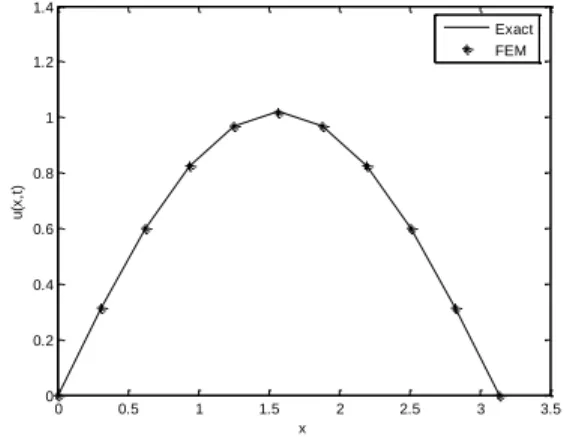
Fig. 3 Comparison of FEM with Exact Solution

4. Results and Discussion

In Table 1, a comparison of FEM solution with exact solution along with absolute errors is presented. It can be observed that computed values are very close to exact values and corresponding errors are very small. In Figure 3 both FEM and exact solutions are plotted. Dots represent FEM solution for different nodal values and continuous curve represents the exact solution for the test problem. It is clear from the plot that solution obtained by developed scheme is approximately equal to exact solution.

5. Conclusion

A Galerkin based Finite Element Model for linear second order one dimensional Inhomogeneous wave equation has been developed. Accuracy of the developed scheme has been analyzed by solving a test problem and comparing computed values with exact solutions.

6. References

[1] William H. Press, Saul A. Teukolsky, William T. Veltering, Brian P. Flannery. (2007).

Numerical Recipes.3rd ed. Cambridge

University Press.

[2] Gerald C. F. & Wheatly P. O. (2005). Applied Numerical Analysis. 6th ed. Pearson Education Inc.

[3] Julien Diaz, Marcus J. Grote. (2009). Energy Conserving Explicit Local Time Stepping for Second Order Wave Equations. SIAM J. Sci. Comput Vol.31 No 3 pp.1985-2014.

[4] H-.Kries, N.A. Peterson, J. Ystrom. (2002). Difference Approximations for the Second Order Wave Equation. SAIM J. Numer.Anal.,40 pp1940-1967.

[5] Burden, R.L. & Faires, J.D. (2001) Numerical Analysis, 7th ed., Thomson Brooks/Cole.

[6] J. D. (2006). Hoffman. Numerical Methods for Engineers and Scientists.2nd ed. Marcel Dekker, inc.

[7] Reddy J.N. (2006). An Introduction to the Finite

Element Method. 3rd ed., McGraw Hill

International Ed.

[8] Sastry S.S. (2005). Introductory Method of Numerical Analy sis. 4th ed. Prentice-Hall of India Private Ltd.