Sharif University of Technology
Scientia IranicaTransactions E: Industrial Engineering www.scientiairanica.com
Supply chain network design for deteriorating items
with discount on transportation cost
M. Hajian Heidary, S.M.T. Fatemi Ghomi
and B. Karimi
Department of Industrial Engineering, Amirkabir University of Technology, 424 Hafez Avenue, Tehran, 1591634311, Iran. Received 26 January 2014; received in revised form 23 August 2014; accepted 17 November 2014
KEYWORDS Supply chain network design;
Deteriorating items; Discount;
Improved meta-heuristic algorithm.
Abstract. Distribution of deteriorating items is dierent from that of other items. This issue leads distributors to transport in lower volumes. On the other hand, one of the mechanisms that attract buyers to purchase items is discount; although a larger amount of order has a lower price for one item, it has a higher risk of deterioration. Despite the importance of the issue, previous researches on deteriorating items did not consider discount conditions in designing supply chain network. Hence, in this paper, balancing the cost of ordering and the cost of deterioration, with consideration of discount, through a new model is studied. The problem is solved for numerical examples with an improved meta-heuristic method composed of Simulated Annealing (SA) and Genetic Algorithm (GA) and the results are reported. Furthermore, a heuristic method for small scale problems is represented and compared with the introduced algorithm to analyze performance of the method. Finally, results show a signicant dierence between the costs of the models (with discount and without it).
© 2015 Sharif University of Technology. All rights reserved.
1. Introduction
In recent years, many researchers are attracted to issues related to supply chain management [1]. One of the most important problems in this eld is the proper design of supply chain. Supply Chain Network Design (SCND) problems are extended in dierent ways. These extensions include considering dierent types of facilities and multi echelon networks and multiple types of products, stochastic and dynamic parameters of demands and costs [2].
There are many studies which investigate design-ing supply chain network. Jayaraman [3] investigated the simultaneous relationship between management of inventory, facility location, and determination of transportation policy. The author suggested an in-tegrated model for designing a distribution network which showed correlation of these three elements. Also,
*. Corresponding author. Tel.: +98 21 64545381; Fax: +98 21 66954569
a mathematical model of mixed integer programming was proposed whose objective function was minimizing the total distribution costs related to the three decision variables (facilities location, inventory, and dierent options of transportation). Jayaraman and Pirkul [4] studied the problem of multi producers and multi-commodity facility location with the goal of minimizing total xed costs of establishment of facilities and variable costs of dispatching and processing the com-modities. Also, a heuristic Lagrangian-based method was proposed in this research. Ross and Jayaraman [5] worked on a type of problem which deals with design-ing the distribution network with multiple products, one producing center, multiple Distribution Centers (DCs), cross docking, and multiple markets. To solve this problem, simulated annealing algorithm is used. Garrido and Miranda [6] suggested an approach to integrate inventory control decisions in general models of facility location. In this research, demand is assumed stochastic, and a nonlinear mixed integer model and a heuristic algorithm are proposed to solve the problem.
Amiri [7] investigated designing a distribution network in supply chain. For this purpose, a facility location model with single product and multiple manufacturers was extended. The facilities had multi-level capacity and the model determined the optimum level of capac-ity. A heuristic approach was proposed to solve the problem.
Deteriorating items such as foods, drugs, lms, or drinks are damageable, perishable, or vaporizable and have typically an expiration date [8]. Sometimes dete-riorating items cause time-constraints for distribution network in supply chain.
Many researchers have worked on this eld. Ghare and Schrader [9] were the pioneers of this eld. In their research, the eect of decaying products on the function of inventory systems was explained. Covert and Philip [10] designed an inventory control model for deteriorating items with variable deteriorating rates and supposed that shortage was not allowed. In their study, deteriorating rate was considered based on Weibull density function. Wee [11] proposed a model for determining the Economic Production Quantity (EOQ) for deteriorating items with xed production rates and loss of shortage. Wee and Yang [12] suggested a multi-level mathematical model for deteriorating items. The model, economic order quantity in wholesale and retail, was concerned with the objective of simultaneous minimization of inventory costs at each level. Sarker et al. [13] designed a sup-ply chain network for deteriorating items considering ination rate and delay in payment and shortage with the goal of determining optimum ordering policy for customers. Tarantilis and Kiranoudis [14] proposed a meta-heuristic approach for routing distribution of deteriorating foods. In this research, a solution for the problem of fresh milk distribution in Greece was proposed. Law and Wee [15] suggested an inventory-production model for deteriorating and ameliorating items from the viewpoints of customer and producer. Deteriorating and ameliorating rates were calculated based on Weibull distribution. They developed a heuristic method to achieve the optimal solution. Chen and Chen [16] proposed an inventory control policy with periodic review. The objective function consid-ered simultaneous replenishment planning and discount for deteriorating items. Periodic review was compared with xed order quantity in the research. The problem was formulated as a dynamic planning problem and was solved with numerical searching techniques. The results showed that periodic review was better than xed order quantity. Begum et al. [17] proposed an EOQ model for deteriorating items considering unit production cost, nonlinear demand, and short-age.
On the other hand, to attract more customers, vendors utilize some mechanisms such as discount on
price for a large amount of order. Some researchers considered discount in designing supply chain. Tsao and Lu [18] investigated designing a supply chain with considering cost discount. Also some researchers, such as Tang and Yang [19] and Tang et al. [20], studied supply chain network design for deteriorating items; but, there seems to be a gap in designing supply chain network for deteriorating items with consideration of discount.
The paper is structured as follows. In Section 2, SCND for deteriorating items is modeled. Section 3 introduces an improved meta-heuristic algorithm composed of simulated annealing algorithm and genetic algorithm. In Section 4, a numerical example is surveyed and the two methods (SA and GA) are compared. Finally, conclusions are drawn in Section 5. 2. Development of the model
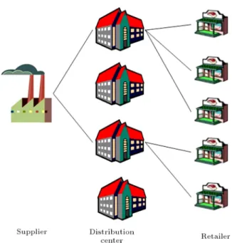
The model, developed in this paper, considers a three-stage supply chain network consisting of a supplier and many customers and many DCs. Any customer's demand could be assigned to any DC, if a DC has enough inventory. Schematic of the supply chain is illustrated in Figure 1.
The main objective, in this paper, is cost reduc-tion for all parts of the supply chain. Main variables are decision making about establishing a DC, assigning demand, and selecting a price level for that DC. 2.1. Assumptions and notations
In the model, following assumptions are considered: 1. DCs have sucient inventory for a specic item; 2. The rate of discount announced by any DC is
dierent;
3. Shortage is not allowed;
4. Deterioration occurs when the items arrive at the DCs;
5. Deterioration rate is constant and called (is small). Notations are dened as follow:
Ij(t) Inventory level of DC j
ai Demand rate of customer i
Ai Fixed cost of each order
Qj Amount of each order
Ti Planning period for customer i
T Cj annual inventory cost
h Fixed holding cost per unit of item p Fixed deterioration cost per unit of
item
cjn The shipment cost that DCj chooses
from price level n
fj The xed cost of locating a DC at
candidate site j
xj = 1 If potential site j is chosen and 0,
otherwise
yij = 1 If demand at customer i is assigned to
DCj and 0, otherwise
zjk= 1 If DCj chooses price level k and 0,
otherwise
dj;n nth quantity break point for DC j.
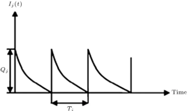
Some notations are related to inventory manage-ment; to illustrate those parameters, Figure 2 depicts inventory level at DCj:
2.2. Model
After introducing variables and parameters, the prob-lem can be dened as locating DCs and determining the assignment of demands of retailers to them so as to satisfy the demands of the retailers. Any retailer's demand could be assigned to any DC, and if a DC has enough inventory, it can support all the retailers. Each of the DCs announces a price level from the levels dened for discounting.
Figure 2. Inventory level at DCj.
Suppose that Dj is dened as the total demand
rate served by DCj, or Dj =Piai.
Transportation cost with consideration of dis-count is:
cjn=
8 > > > > > > > < > > > > > > > :
cj1; Dj< dj1
cj2; dj1 Dj dj1< dj2
...
cjn; dj;n 1 Dj dj;n 1< dj;n
(1)
Note that discount is incremental. For the incremental discount policy, the discount applies only for quantities exceeding the break points. Inventory change in t is equal to the summation of item deterioration and consumption of the item. This means:
dIj(t)
dt + Ij(t) = Dj;
0 t Tj: (2)
Similar to Dj, suppose that c0j is the shipment cost
that DCj nally chooses to place from k price level.
Therefore: T Cj =hD2Tj
j e
Tj T
j 1+ATj j
+p(Qj DjTj)
Tj + c
0 jQTj
j: (3)
In Eq. (3), the rst term is holding cost, the second term is the cost of placing order, the third term is the deterioration cost, and the fourth term is the shipment cost.
Holding cost and deteriorating cost, used in Eq. (3), are obtained as follows:
Inventory level at t can be obtained as follows: I(t) = e RdtZ DeRdt+ dt + c
= c tZ Detdt + c= e t Det+ c
= D + e tc:
(3.1) Using boundary condition (I(T ) = 0):
I(t) =D
eT et
et
;
0 t T: (3.2)
h Z T
0 I(t)dt = h
Z T 0
D
eT et
et
dt = hD
Z T
0
e(T t) 1dt
= hDeTZ T 0 e
tdt hD
T = hD2eT 1 e T hD
T = hD2 eT 1 hD
T
= hD2 eT T 1: (3.3)
The amount of deteriorating is the dierence between amount of order and amount of demand in period T . Thus, deteriorating cost can be obtained from multiplying p by this amount.
Solving Eq. (3) is dicult because of the existence of exponential functions; hence, using Taylor extension and neglecting the third and larger powers of and for small values of , the following term can be used instead [21]:
e=2 + t
2 t: (4)
By substituting Eq. (4) in Eq. (3), and then taking derivative from Eq. (3) (convexity of the Eq. (3) is proved in Appendix A), optimal annual inventory cost will be:
T C j =
s
2DjAj
h + p + c0 j + c
0
jDj: (5)
Now with the assumption that Dj and c0j are known,
the model is formulated as follows:
minX
j
fjxj+
X
i2I
ai
X
k
cjkzjk
! yij
!
+sX
i2I
2aiAj(h + p +
X
k
cjkzjk)yij
: Subject to:
X
j
yij = 1; i 2 I
yij xj; i 2 I
zjk xj
"zj1< Dj dj;1zj;1
dj;1zj;2< Dj dj;2zj2
...
dj;n 1zjn< Dj< Mzjn
xj; yij; zjk2 f0; 1g; (6)
where M is a big number.
The objective function minimizes the sum of deterioration cost, holding cost, xed cost of estab-lishing DCs, order cost, and transportation cost. The rst constraint ensures that demand at customer i is assigned to one of the DCs. The second and the third constraints guarantee that if a DC is not established, yij and zjk will be equal to zero. Other constraints
show dierent levels of prices with respect to discount. The rst term of the objective function and the rst and second constraints can be considered as a UFLP. UFLP is an Np-hard problem [22]. The problem has extra constraints and is nonlinear which leads to a more complex problem. Hence, meta-heuristic methods are developed to solve the problem.
3. Improved meta-heuristic algorithm
Meta-heuristic methods are generally divided into two classes: constructing and improving methods. Con-structing methods rst generate the initial solutions and then improve them, but the improving methods need initial solutions to improve them to gain the best possible solutions.
One of the most applied meta-heuristic methods is simulated annealing. This improving method is a generic probabilistic one for the global optimization problem of locating a good approximation to the global optimum in a large search space. Simulated annealing is a process wherein the temperature is reduced slowly, starting from a random search at high temperature, eventually becoming a pure greedy descent as it ap-proaches zero temperature.
This notion of slow cooling is implemented in the SA algorithm as a slow decrease in the probability of accepting worse solutions as it explores the solution space [23]. Accepting worse solutions is a fundamental property of meta-heuristics, because it allows for a more extensive search for the optimal solution.
Another method, frequently used in the literature, is genetic algorithm. This algorithm, as an improving method, is routinely applied to generate acceptable solutions to optimization and search problems [24]. In a genetic algorithm, a population of candidate solutions to an optimization problem is evolved toward better solutions. Each candidate solution has a set of properties which can be mutated and altered; the evolution usually starts from a population of initial
solutions. In each generation, the tness of every individual in the population is evaluated; the more tted individuals are stochastically selected from the current population. Then, using mutation, a new population is created. It is, then, used in the next iteration of the algorithm.
To achieve better solutions, sometimes it is re-quired to combine two or more meta-heuristics. In this paper, an improved meta-heuristic algorithm with two parts is developed. The SA outputs are applied as the initial solutions for GA. Using these initial solutions and other mechanisms, such as mutation and crossover, GA improves initial solutions and reaches better solu-tions for the problem. Details of the improved method are discussed below.
The rst part of the improved algorithm is SA. SA is applied to generate initial solutions for the GA. After determining the initial and the nal temperatures for the algorithm, the cooling mechanism is selected as a geometric procedure. The stopping condition is dened as reaching a proper number of iterations (MaxIt). Eq. (7) shows a geometric cooling function. Alpha is the geometric multiplier and Tf and T0 are the initial
and nal temperatures.
Alpha = (Tf=T0)^(1=Maxlt): (7)
Also, to diversify movement in the solution space, usually a worse solution is accepted by a probability. In this paper, the probability function is applied based on Eq. (8). If a random number between zero and one is smaller than this probability, the new solution is accepted as the current solution.
P = exp ((bestcost cost)=T ) : (8)
The main loop of the algorithm is introduced in Box I. This algorithm is executed for the number of the initial solutions required to run GA. Initial solutions by SA are better than the randomized ones.
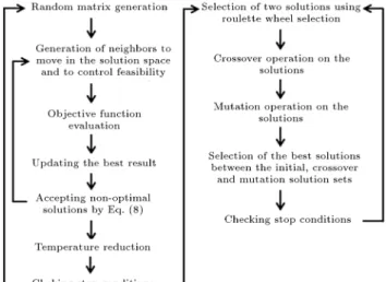
Figure 3. The meta-heuristic algorithm.
Genetic algorithm applied in the second step of the algorithm is shown in Box II.
Thus, utilizing the initial solutions from SA and improving them by GA helps to gain better global solutions with a better value for objective function. Figure 3 briey shows the improved algorithm.
In the algorithm shown in Box II, as mentioned above, genetic algorithm is used to improve the results of SA algorithm. In the next section, results of some numerical examples are surveyed.
4. Numerical example
As mentioned before, the problem, studied in this paper, is determining supply chain features, such as location of DCs and assigning demands to each estab-lished DC. The conditions considered for the supply chain are deterioration of the items and discount on transportation costs.
The supply chain consists of 3 echelons, one supplier and some DCs and retailers. Some problem instances, consisting of small, medium, and large size For each iteration
Construct an empty matrix and ll it with random variables
// Using it, locating the DCs and selecting the levels of the price can be performed
// Dimensions of the matrix are related to the number of potential DCs and the number of // retailers, and also the number of levels announced for discount.
Use the neighborhood mechanisms to move in the solution space and control the feasibility of the new solution,
// Shift and swap the mechanism used in this section Calculate the objective function for this solution
Substitute this solution with the best solution rec- ognized so far, under the following conditions: // if the objective function of new solution is better than the best objective function, found so far // if the above condition has not occurred, with the probability equal to Eq. (8), substitution is allowed Temperature= Temperature Alpha
End
For each iteration
Use roulette wheel method to select two initial solutions Perform crossover on the two solutions selected
// Hold the results in a set (set 1) // Check feasibility
Perform mutation on some of the initial solutions // Hold the results in a separate set (set 2) // Check feasibility
From initial solutions, set 1 and set 2, select the best solutions with the better values for objective function
End
Box II
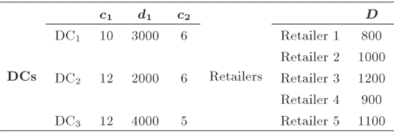
Table 1. Data for the small scale problem instances.
DCs
c1 d1 c2
Retailers
D
DC1 10 3000 6 Retailer 1 800
Retailer 2 1000
DC2 12 2000 6 Retailer 3 1200
Retailer 4 900
DC3 12 4000 5 Retailer 5 1100
Table 2. Results from solving the small size problem instances.
SA GA IMA
Objective function 75859 75859 75859
problems, are tested with the improved algorithm. To show performance of the improved algorithm, it is applied on each of the problem instances. The contribution of the two portions of the proposed algo-rithm in solution quality is shown. In these problems, the deterioration rate is 0.01, deterioration cost is 5, holding cost is 10 (per unit), xed cost of each order is 500, and establishing cost for each DC is 10000.
First, a small problem is studied. This problem consists of one supplier, three DCs and ve retailers; each DC has two separate levels of price. Data for this problem is presented in Table 1.
Under an identical time and number of iterations, Table 2 shows the results from the SA, the GA, and the Improved Meta-heuristic Algorithm (IMA).
According to the results of the algorithms, only the rst DC is economic to establish and others are not chosen by the algorithms.
It is very dicult to solve the problem, manually, because the number of cases prevents calculation with-out software. But, there is an easy way to approach the answer which is proposed below.
Lemma 1. In addition to the results from the meta-heuristics, for small sizes and under the assumption that holding cost and deterioration cost are negligible, some results can be guessed. For each DC, there are two prices and one break point of discount.
There are three major components of the problem that impact the solutions. The rst component is the price of the rst level of discount (c1). The second
component is the dierence between price of the second and the rst levels of discount (c1 c2). The third
component is the break point (d). These components, together, determine that which DCs can be established. Smaller values for c1, d and larger values for c1 c2
are desirable. Hence, the index below can show the desirability for the choice of DCs.
Vj= ccj1 cj2
j1 dj; cj1> cj2: (9)
Based on the above points, the steps below help to solve the problem.
Find the smallest price in the rst level of discount between all DCs and name break point of discount in this DC (DCl): dl.
If the sum of demands is larger than dl, order dl
from DCl. For the other DCs, two cases can happen:
1. Break point of discount of other DCs is larger than dl. Order from DCl;
2. Break point of discount of other DCs is equal or smaller than dl. With Vj, select the next DC to
order.
As an example, it is shown that just DC1 should
be established from three DCs explained in the small instance problem. For this problem, Lemma 1 is applied below.
The smallest price in the rst level of discount between all DCs is 10 in DC1, thus: dl = 3000.
In DC2, break point is 2000, and in DC3 it is
4000. Thus, we use the index which is explained. Vj's
are calculated as: V1 = 0:000133, V2 = 0:00025, V3 =
0:000146. Hence, choose DC1 for the remained orders.
This lemma cannot be used for the large problems and problems with many discount break points.
The next problem instances, considered in this paper, show performance of the proposed algorithm in a larger size. In this scale of problem, 30 DCs and 100 retailers comprise the supply chain. Also three levels of price are considered.
Parameters of the problem are determined as below:
- Values for retailer demands are uniformly drawn from [200, 400];
- Values for the rst level of transportation cost are uniformly drawn from [5, 8];
- Values for the second level of transportation cost are uniformly drawn from [9, 12];
- Values for the third level of transportation cost are uniformly drawn from [13, 15];
- Values for the rst break point of discount are uniformly drawn from [800, 1300];
- Values for the second break point of discount are uniformly drawn from [1300, 2200];
- Values for other parameters are the same as those for the small size problem.
Results of solving the problem with 3 meta-heuristic algorithms are presented in Table 3. SA solves the problem with T0 = 1000 and Tf = 0:01, and the
number of iterations in each temperature is 100. GA is applied to the problem with crossover rate of 0.8 and mutation rate of 0.3. The improved algorithm rst solves the problem with 5 matrices which is made by SA. Under an identical time, Table 3 gives the results from each method.
The initial solution has intensive eect on the results of simulated annealing algorithm, and if there is not a good initial solution for SA, nal results may not be suitable. In this paper, because of the general denition of the problem, and random selection of initial solution, nal SA results are not desirable and must be combined with GA for improvement. The combination is performed properly and makes remarkable improvement on the output of SA. In other words, contribution of the GA in improvement
Table 3. Results from 3 meta-heuristic algorithms to solve large scale problems.
SA GA SA-GA
Objective function 618740 192740.4 147295
Time (sec) 32 21 46
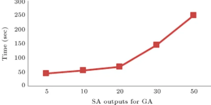
Table 4. Eect of the number of outputs of SA, used to run GA, on the time and quality of solutions.
SA outputs used for GA
Objective function
Time (Sec)
5 147295 46
10 146261 55
20 141711 68
30 130909 145
50 130909 250
of the SA results is about 69% and the combination of SA with GA also improves the results of GA by 23%.
Table 4 shows sensitivity analysis of output num-bers of solutions obtained by SA used as GA initial solutions. The table shows the eect of using outputs of SA for GA. As the number of SA outputs increases, solutions will be better, but execution time increases. This issue is shown, graphically, in Figures 4 and 5.
Results indicate that the best solution tends to assign demands to the minimum possible number of DCs. On the other hand, costs, such as deterioration, holding, and establishing costs, balance the number of established DCs.
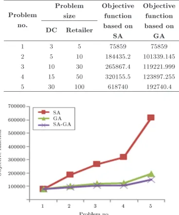
Improved algorithm is used to evaluate some other problem instances. Results are shown in Table 5.
According to the results of Table 5, performance of the improved algorithm is depicted in Figure 6.
Figure 4. Eect of dierent numbers of SA outputs, used for GA, on the objective function.
Figure 5. Eect of dierent numbers of SA outputs, used for GA, on the running time.
Table 5. Results from meta-heuristic algorithms to solve some problem instances. Problem
Problem Objective Objective Objective % Improvement % Improvement no.
size function function function of IMA of IMA
DC Retailer based on based on based on over SA over GA
SA GA SA-GA
1 3 5 75859 75859 75859 -
-2 5 10 184435.2 101339.145 91574.92 50 9
3 10 30 265867.4 119221.999 104433.4 61 12
4 15 50 320155.5 123897.255 103004.7 68 17
5 30 100 618740 192740.4 147295 76 24
Figure 6. Comparison between results of algorithms in dierent problem instances.
5. Conclusion and future research
Supply chain management is developed in many in-dustries as a concept and is performed, properly, at those industries. One of the most important parts of actualization of this concept is designing a network for the supply chain. To consider more aspects of real world in designing the supply chain, sometimes dis-count is announced on price. Previous studies did not consider discount in designing supply chain networks for transporting deteriorating items, and therefore, there were no solutions for such problems. Also, tuning the parameters of algorithms and designing an improved algorithm, based on the conditions of such problems, to solve the model are another contributions of the paper.
In this paper, rst, a supply chain for deteri-orating items was modeled, and then, it was solved by three meta-heuristics: SA, GA, and a combination of them. GA performed better than SA for prob-lems dened based on the model; additionally, the proposed algorithm performed better than the others. SA, because of its nature and use of random initial solution, performed inappropriately; hence, application of an accessory method seems reasonable in addition to SA. Also, for the small size problems, a manual approach was proposed in the paper which helped to
reach the solution. Results of the improved algorithm showed reasonable expectations, such as assigning more demands to DCs, announcing lower prices, and lower break points of discount, from the problem. As an area for future research, study of the proposed model in real world cases, considering shortage with ecient algorithms, can be recommended.
References
1. Hajiaghaei-Keshteli, M. \The allocation of customers to potential distribution centers in supply chain net-works: GA and AIA approaches", Applied Soft Com-puting, 11, pp. 2069-2078 (2011).
2. Sadjady, H. and Davoudpour, H. \Two-echelon, multi-commodity supply chain network design with mode se-lection", Lead-Times and Inventory Costs, Computers & Operations Research, 39, pp. 1345-1354 (2012).
3. Jayaraman, V. \Transportation facility location and inventory issues in distribution network design: An in-vestigation", International Journal of Operations and Production Management, 18(5), pp. 471-494 (1998).
4. Pirkul, H. and Jayaraman, V. \A multi commodity multi plant capacitated facility location problem: For-mulation and ecient heuristic solution", Computers & Operations Research, 25(10), pp. 869-878 (1998).
5. Jayaraman, V. and Ross, A. \A simulated annealing methodology to distribution network design and man-agement", European Journal of Operational Research, 144, pp. 629-645 (2003).
6. Miranda, P.A. and Garrido, R.A. \Incorporating in-ventory control decisions into a strategic distribution network design model with stochastic demand", Trans-portation Research Part E, 40, pp. 183-207 (2004).
7. Amiri, A. \Designing a distribution network in a supply chain system: Formulation and ecient so-lution procedure", European Journal of Operational Research, 171, pp. 567-576 (2006).
8. Maihami, R. and NakhaiKamalabadi, I. \Joint pricing and inventory control for non-instantaneous deterio-rating items with partial back logging and time and price dependent demand", International Journal of Production Economics, 136, pp. 116-122 (2012).
9. Ghare, P.M. and Schrader, S.F. \A model for expo-nentially decaying inventory", Journal of Industrial Engineering, 14, pp. 233-243 (1963).
10. Covert, R.B. and Philip, G.C. \An EOQ model with Weibull distribution deterioration", AIIE Transac-tions, 5, pp. 349-354 (1973).
11. Wee, H.M. \Economic production lot size model for deteriorating items", Computer & Industrial Engineer-ing, 6, pp. 309-317 (1993).
12. Wee, H.M. and Yang, P.C. \Economic ordering policy of deteriorated items for vendor and buyer: An inte-grated approach", Production Planning and Control, 11, pp. 474-480 (2000).
13. Bhaba, R., Sarker, A.M.M. and Jamal, Shaojun W. \Supply chain models for perishable products under ination and permissible delay in payment", Comput-ers & Operations Research, 27, pp. 59-75 (2000).
14. Tarantilis, C.D. and Kiranoudis, C.T. \A meta-heuristic algorithm for the ecient distribution of perishable food", Journal of Food Engineering, 50, pp. 1-9 (2001).
15. Law, S.T. and Wee, H.M. \An integrated production-inventory model for ameliorating and deteriorating items taking account of time discounting", Mathemat-ical and Computer Modeling, 43, pp. 673-685 (2006).
16. Chen, J.M. and Chen, L.T. \Periodic pricing and replenishment policy for continuously decaying inven-tory with multivariate demand", Applied Mathematical Modeling, 31, pp. 1819-1828 (2007).
17. Begum, R., Sahu, S.K. and Sahoo, R.R. \An EOQ model for deteriorating items with Weibull distribution deterioration, unit production cost with quadratic de-mand and shortages", Applied Mathematical Sciences, 4(6), pp. 271-288 (2010).
18. Tsao, Y.C. and Lu, J.C. \A supply chain network de-sign considering transportation cost discounts", Trans-portation Research Part E, 48, pp. 401-414 (2012).
19. Tang, K. and Yang, C. \A distribution network design model for deteriorating item", International Journal of Logistics Systems, 4, pp. 366-383 (2008).
20. Tang, K., Yang, C. and Yang, J. \A supply chain network design model for deteriorating items", In-ternational Conference on Computational Intelligence, China (2007).
21. Rau, H., Wu, M.Y. and Wee, H.M. \Integrated in-ventory model for deteriorating items under a multi-echelon supply chain environment", International Journal of Production Economics, 86, pp. 155-168 (2003).
22. Gabor, A.F. and Ommeren, J.K.C.W.V. \A new approximation algorithm for the multilevel facility lo-cation problem", Discrete Applied Mathematics, 158, pp. 453-460 (2010).
23. Meysam Mousavi, S. and Tavakkoli-Moghaddam, R. \A hybrid simulated annealing algorithm for location
and routing scheduling problems with cross-docking in the supply chain", Journal of Manufacturing Systems, 32, pp. 335-347 (2013).
24. Yu, Y., Hong, Z., Zhang, L.L., Liang, L. and Chu, C. \Optimal selection of retailers for a manufactur-ing vendor in a vendor managed inventory system", European Journal of Operational Research, 225, pp. 273-284 (2013).
Appendix A
Here, convexity of Eq. (3) is proved. The rst deriva-tive of the function (rewritten) is as follows:
T C0
j = hD2j e
Tj Tj 1
T2 j
!
+hD2j
eTj
Tj Aj T2 j pQj T2 j c0 jQj
T2 j :
And the second derivate of the function (rewritten) is as follows:
T C00
j = hD2j
Tj(eTj ) 2(eTj Tj 1)
T3 j
!
+hD2j 2eTjTjT2eTj +
j ! 2Aj T3 j 2pQj T3 j 2c0 jQj
T3 j :
It can be rewritten as: T C00
j =hD2j
eTj(2T2
j 2Tj+ 2) 2
T3 j ! 2Aj T3 j 2pQj T3 j 2c0 jQj
T3 j :
It can be expressed that the convexity of function can be proved through the following relation:
T C
j = hD2j eTj((1 + Tj)2+ 1) 2
2Aj+ 2pQj+ 2c0jQj:
Tj and are positive, then:
eTj((1 + T
j)2+ 1) 2 0:
Thus for the small values of , T Cj is convex. Hence,
derivation and use of minimum function as objective function are rational.
Biographies
Mojtaba Hajian Heidary received his MSc degree in Industrial Engineering from Amirkabir University of Technology, Tehran, Iran, in 2013. His research interests are: supply chain management, simulation and mathematical modeling.
Seyyed Mohammad Taghi Fatemi Ghomi was born in Ghom, Iran, in 1952. He received his BS degree in Industrial Engineering from Sharif University, Tehran, Iran, in 1973, and a PhD degree in Indus-trial Engineering from Bradford University, UK, in 1980. From 1980 to 1983, he worked as a Planning and Control Expert in the group of construction and cement industries within the Organization of National
Industries of Iran. Also, in 1981, he founded the Department of Industrial Training in the aforemen-tioned organization. He joined Amirkabir University of Technology, Tehran, Iran, as a faculty member in 1983. He is now Professor at the Department of Industrial Engineering, Amirkabir University of Technology. His research and teaching interests include: stochastic activity networks, production planning and control, scheduling, queuing systems, and statistical quality control.
Behrooz Karimi received his PhD degree in Indus-trial Engineering, in 2002, from Amirkabir University of Technology, Tehran, Iran, where he is now Associate Professor. His areas of research include: supply chain planning, scheduling and simulation.