Sharif University of Technology
Scientia IranicaTransactions A: Civil Engineering www.scientiairanica.com
Evaluation of the static and seismic active lateral earth
pressure for c
soils by the ZEL method
A. Keshavarz
and Z. Pooresmaeil
School of Engineering, Persian Gulf University, Bushehr, Iran.
Received 9 November 2014; received in revised form 11 April 2015; accepted 2 June 2015
KEYWORDS Zero extension lines; Static;
Seismic; Active;
Lateral earth pressure; Retaining walls; Non-associated.
Abstract. The method of Zero Extension Lines (ZEL) has been used to evaluate the static and seismic active lateral earth pressure on an inclined wall retaining c backll. The equilibrium equations along the zero extension lines have been solved using the nite dierence method. A computer code is prepared to analyze the retaining wall, calculate the ZEL network and the distribution of the active lateral earth pressure behind the retaining wall. The total active force on the retaining wall was dened as the lateral earth pressure coecients due to the soil unit weight, the surcharge, and the soil cohesion. The variations of the active lateral earth pressure coecients with changes in dierent parameters, such as the inclination of the earth and wall, the friction angle of the soil, the adhesion of the soil-wall interface, the horizontal and vertical pseudo-static earthquake coecients, have been obtained. The results have been obtained for soils with associated and non-associated ow rules. The eect of the dilation angle has also been considered. The results obtained in this study are very close to those of other methods and conrm that the ZEL method can be successfully used to evaluate the lateral earth pressure of retaining walls.
© 2016 Sharif University of Technology. All rights reserved.
1. Introduction
Many dierent methods are provided to evaluate the active lateral earth pressure on the retaining wall. Rankin and Coulomb are the common methods. Stress characteristics [1,2] or slip lines method, limit analysis method [3,4], Rankine's conjugate stress concept [5], and slice analysis method [6] are also used to evaluate the lateral earth pressure. Zero Extension Lines (ZEL) method is one of the methods that is capable of analyzing the stability of retaining walls under general conditions in static and seismic conditions. This method was rst used by Roscoe [7] to solve static and dynamic problems of retaining walls. In 1971, James and Bransby [8] used ZEL method to
*. Corresponding author. Tel/Fax: +98 77 33440376 E-mail addresses: [email protected]; and amin [email protected] (A. Keshavarz); [email protected] (Z. Pooresmaeil)
predict the strain patterns behind retaining walls. Habibagahi and Ghahramani [9] presented an earth pressure theory based on the simple ZEL eld to predict stress patterns in the backll behind a vertical wall. Anvar and Ghahramani [10] derived the equilibrium equations along the ZEL and presented the application of ZEL method. Jahanandish [11] developed a theory regarding the ZEL method and derived the equilibrium equations along zero extension lines for axial symmetry. Furthermore, ZEL method has also been used to study the stability of slopes [12], analyze three-dimensional stability of soils [13], predict the behavior of dense frictional soils [14], and evaluate bearing capacity of soils and foundations and dynamic lateral pressure of retaining structures [15-17]. Veiskarami et al. [18-20] used this method to predict the bearing capacity of foundations and load-displacement behavior of shallow foundations considering the stress level eect.
Many available methods evaluate lateral earth pressure on the retaining walls by using the assumption
of the associated ow rule, although `Real' soils have a non-associated ow rule and the dilation angle is smaller than the friction angle [21]. One of the advantages of ZEL method is that in this method, soil can be associative or non-associative. Therefore, by using the ZEL method, the eect of the dilation angle can be evaluated. Lee and Herington [22] evaluated the passive earth pressures for non-associated ow rules by a theoretical study. Shiau and Smith [23] studied, numerically, the eect of non-associated ow rule on the passive earth pressure. Benmeddour et al. [21] provided passive and active lateral earth pressure coecients due to the soil unit weight for the soil with dilation angle equal to zero. They studied the inuence of non-associativity by a numerical method and modifying values of the soil friction angle and cohesion.
Moreover, ZEL method does not have the limita-tion of assuming the shape of the rupture surface. By using this method, the failure zone is determined after analyzing the retaining wall. ZEL method analyzes geotechnical problems in the strain eld. When the soil is assumed as associative soil, i.e. the friction angle of the soil is equal to its dilation angle, ZEL method is similar to the stress characteristics or slip lines method. The ZEL method has been used in this paper to evaluate the seismic stability of retaining walls for non-associated and non-associated ow rules and propose the lateral earth pressure coecients. Although Habiba-gahi and Ghahramani [9] developed the ZEL for static lateral earth pressure, they used the simple ZEL led and developed the method for sands. This study develops the ZEL method for the active lateral earth pressure for c soils in seismic case. Consideration of the eect of dierent parameters of the soil and retaining wall, especially the soil dilation angle, is one of the advantages of this study. Also, the lateral earth pressure coecients due to the soil unit weight, surcharge, and soil cohesion have been provided for non-associative soil.
2. Theory
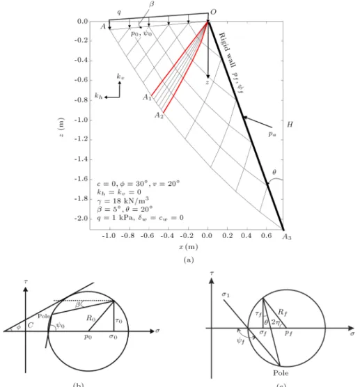
The geometry of the retaining wall in the active case has been shown in Figure 1(a). The surcharge q is applied on the ground surface. The ground surface makes an angle with the horizontal direction and the wall angle with the vertical direction is . The height of the retaining wall is H. The positive directions of the and are shown in Figure 1(a).
2.1. Assumptions
1. The backll soil is considered as a c soil and follows the Mohr-Coulomb yield criterion, where c is the cohesion in kPa and is the internal friction angle in degree;
2. The unit weight of the soil mass is assumed equal to in kN/m3;
3. The friction angle in the interface between soil and wall is considered as w in degree;
4. The adhesion of the soil-wall interface is assumed cw in kPa;
5. The principle of superposition is valid for static and seismic analyses;
6. The retaining wall problem is considered plane strain and two dimensional.
2.2. Boundary conditions
Analyzing the problem requires knowing the boundary conditions along the ground surface and the retaining wall. The boundary conditions are explained in the following sections.
2.2.1. Along the ground surface
To calculate the coordinates (x; z) of the points on the ground surface, a length of L is considered on this boundary and it is divided into n divisions. According to Figure 1(a), the coordinates of the point number i on the ground surface can be calculated as:
xi= Ln(i 1) cos ; zi= xitan ; (1)
where is the ground angle with horizontal direction. As mentioned before, the vertical stress q is applied on the ground surface. So, the normal and shear stresses for the points on the ground are obtained as:
0= q cos [(1 kv) cos khsin ] ;
0= q cos [(1 kv) sin + khcos ] ; (2)
where kh and kv are horizontal and vertical
pseudo-static earthquake coecients.
The Mohr circle of stress on the ground can be shown in Figure 1(b). The average stress on the ground (p0) is obtained from the Mohr circle:
p0=
0+c cos sin
q
(0sin +c cos )2 (0cos )2
cos2 :
(3) Using the Mohr circle of stress, the angle (the angle between "1 and the horizontal axis) on the ground
surface ( 0) can also be calculated as:
if q = 0 : 0= +2
else 0=2 + 0:5
sin 1p0sin(+)
R0
; (4) where:
tan = 1 kkh
Figure 1. The retaining wall problem: (a) Geometry and ZEL network; (b) boundary condition along the ground surface; and (c) boundary condition along the retaining wall.
2.2.2. Along the retaining wall
Assuming the normal and shear stresses on the retain-ing wall, the Mohr circle of stress on this boundary is shown in Figure 1(c). The following equations are derived from this gure:
f = 2 + + ;
f = pf Rfcos 2f;
f = cw+ ftan w; (6)
where f and f are the normal and shear stresses on
the retaining wall, respectively. Then, the angle on the wall ( f) can be calculated from Eq. (6):
f =2 +
+0:5
w+sin 1
pfsin w+cwcos w
pfsin +cos
: (7)
2.3. Equilibrium equations along the zero extension lines
By considering the soil shearing in a principal plane for plane strain problem, major and minor principal strain increments do not have the same concept. Therefore, two lines (AP and BP) in the soil element will have the linear strains equal to zero in their directions (Figure 2). AP and BP are called the zero extension lines in minus direction (ZEL ) and plus direction (ZEL+), respectively.
Each point in the soil has four features, x, z, p, and . By solving the equations along the zero extension lines, these features can be determined. As illustrated in Figure 2, the angle between zero extension lines is =2 v, where v is the dilation angle of the soil. The angle of zero extension lines with x axis is . Angle is dened as follows:
= 4
v
2: (8)
Figure 2. The directions of zero extension lines and Mohr circle of the strain [10].
Plus ZEL, PB : dz
dx = tan( + ); (9) Minus ZEL, PB : dz
dx = tan( ): (10) The equilibrium equations along the plus and minus zero extension lines can be written as [10]:
dp + 2(p tan + c)
d + @ @" d"+
= fx(dx tan dz) + fz(tan dx + dz) ;
(11) and along the plus ZEL:
dp 2(p tan + c)
d + @ @"+d"
= fx(dx tan dz) + fz(tan dx + dz) ;
(12) where fxand fzare body forces along the x and z axes
which are dened as kh and (1 kv); d"+ and
d" are the length of the plus and minus zero extension lines, respectively, and:
= 1 sin v sin cos v cos ;
= cos vcos ;
= sin sin vcos cos v : (13) If x, z, p, and of points A and B are known, these values of any point P can be found by writing Eqs. (9)-(12) in the nite dierence form:
xP =ZA ZBtgmp tgmmxAtgmm + xBtgmp; (14)
zP = (xC xB) tgmp + zB; (15)
pP = pB+ A1 Bmp( C B); (16)
P =AA3
4: (17)
The parameters in Eqs. (14)-(17) are dened in the appendix. By using the trial-and-error procedure, a function is written in MATLAB to calculate the unknown parameters (x, z, p, and ) of point P . First, it is assumed that these parameters are equal to the parameters of points A and B on the minus and plus ZEL, respectively. Then, the new parameters of point P can be calculated using Eqs. (14)-(17). This procedure is repeated until the dierence between the new and old parameters of point P is small enough. 2.4. ZEL networks
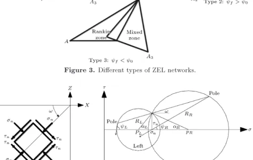
A computer code in MATLAB is provided to analyze the problem. The code starts the calculation from the ground surface. The calculation continues to determine the characteristics of the points on the retaining wall. Three dierent types of ZEL network can arise according to the magnitudes of 0 and f
(Figure 3).
Type 1, f = 0: In this case, the ZEL network
includes Rankin and mixed zones. First, the points in Rankin zone are solved by using the boundary condi-tions on the ground surface and equilibrium equacondi-tions along the ZEL lines. Then, the network in the mixed zone is determined knowing the information on line OA2 and the boundary conditions along the retaining
wall.
Type 2, f > 0: In this case, the ZEL network
Figure 3. Dierent types of ZEL networks.
Figure 4. The soil element on the stress discontinuity line and Mohr circle.
First, the points in Rankin zone are solved by using the boundary conditions on the ground surface and equilibrium equations along the ZEL lines. Now, the relation between and p should be obtained to solve the points in Goursat zone. The p and in the left and right of point O (Figure 1) are dierent and a singularity exists at this point.
Therefore, at point O, dx = dz = 0, and the relation between and p is determined from Eq. (11) as:
if 6= 0; p = c cot + (p0+ c cot )exp
2 sin
cos v ( 0)
;
if = 0; p = cos v2c ( 0) + p0: (18)
Then, the Goursat zone is determined by using the in-formation at the singularity point (point O in Figure 1) and line OA1. Finally, the mixed zone is obtained
similar to Type 1 problem.
Type 3, f < 0: In this case, the Goursat zone
will be removed similar to Type 1 problem and the Rankin and mixed zone will be wrapped. So, a stress discontinuity happens in the stress eld and should be
solved. Lee and Herington [22] provided an algorithm to solve the stress discontinuity. In this study, in order to solve the stress discontinuity, the Lee and Heringtion [22] method has been modied.
An element of the soil has been considered on the discontinuity line (see Figure 4). According to the Mohr circle, shown in Figure 4, the direction of the discontinuity line can be calculated as:
! = 0:5 R+ L cos 1(sin cos( R L));
(19) where, ! is the direction of the discontinuity line and
Rand Lare the angle related to the right and left
sides of the discontinuity line, respectively.
Knowing the left side characteristics of the singu-larity point O (the values on the earth for the rst step) and from Eq. (19), the rst direction (!0) is obtained
and the intersection between the discontinuity line and the ZEL network is calculated. The p and values at the left side of the intersection point are calculated by linear interpolation. Knowing !0, p, and values at
the left side of the intersection point, the stress p and the angle at the right side of the intersection point are obtained. Then, the point on the wall is calculated using the equations along the ZEL lines.
For the next steps, a line with the angle !p (!
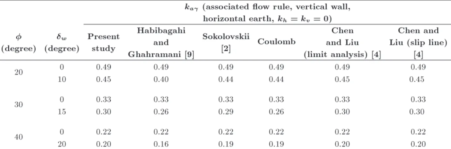
inter-Table 1. Comparison of this study with dierent methods. ka (associated ow rule, vertical wall,
horizontal earth, kh= kv= 0)
(degree) w (degree) Present study Habibagahi and Ghahramani [9] Sokolovskii [2] Coulomb Chen and Liu (limit analysis) [4]
Chen and Liu (slip line)
[4]
20 0 0.49 0.49 0.49 0.49 0.49 0.49
10 0.45 0.40 0.44 0.44 0.45 0.45
30 0 0.33 0.33 0.33 0.33 0.33 0.33
15 0.30 0.26 0.29 0.26 0.30 0.30
40 0 0.22 0.22 0.22 0.22 0.22 0.22
20 0.20 0.16 0.19 0.19 0.20 0.20
section point. The segment of the ZEL network that encounters with the discontinuity line is determined. This segment is divided into ndparts. The information
on these nd points is calculated with the interpolation.
p and at the right side of these nd points are
calculated. Then, the point of the mixed zone should be calculated (point C). The values of x, z, p and of this point can be obtained from Eqs. (14)-(17). The distance between point C and line between the previous intersection point and the point on the wall (for the second step) or in the mixed zone (for the third and the following steps) is calculated. Within these nd points,
the point that has the minimum distance from the line, is selected as the exact intersection point. Knowing the information in the right side of the intersection point, the points in the mixed zone and on the wall can be obtained by using the equations along the ZEL lines. This procedure is repeated until the ZEL network is calculated completely.
3. Results
As mentioned before, the characteristics of the ZEL network points have been determined by a computer code. The average stress on the wall boundary (pf)
has been specied and the f and f distribution along
the retaining wall have been obtained. So, the active lateral earth force has been calculated by integrating stresses and can be dened as [4]:
pa =12H2ka+ qHkaq cHkac; (20)
where ka, kaq, and kac are the active lateral earth
pressure coecients due to the unit weight of the soil, surcharge, and soil cohesion, respectively.
To calculate kaq, the unit weight and cohesion of
the soil are considered zero. Also, the unit weight of the soil and surcharge are assumed zero to obtain kac.
In order to calculate ka, the cohesion of the soil and
surcharge should be assumed as zero. By assuming
this, the problem cannot be solved at the singularity point. Therefore, a small amount of the surcharge (q = 0:01 kPa) is assumed to calculate ka. Then,
to increase accuracy and remove the surcharge eect, ka is modied as:
ka= k0a 2qkHaq; (21)
where, ka is the exact value of the lateral earth
pressure coecient and k0
ais the lateral earth pressure
coecient obtained from analyzing the retaining wall with q = 0:01 kPa.
The lateral earth pressure coecients are ob-tained for the retaining wall in various conditions. Table 1 shows a comparison between the method used in this paper and results of other researchers for ka.
Clearly, this study exactly has the same results as those of Chen and Liu [4]. Furthermore, this study has almost the same results as those of Habibagahi and Ghahramani [9] and the maximum error is 20%. The method of Habibagahi and Ghahramani [9] is based on the simple zero extension line eld that is applied to compute the direction of traction on the zero extension line in a loose sand. Overall, all methods provide the same kavalues for the smooth retaining wall (w= 0)
and a low dierence is observed between ZEL method and other methods for the rough retaining wall. For the wall with w, the dierence between ZEL method
and other methods increases as and wincrease. The
dierence between ZEL method and Coulomb theory, for = 40 and w= 20, is more than other cases.
The seismic ka is shown in Figure 5 for the
associated ow rule (v = ). The eects of the horizontal and vertical pseudo-static coecients have been evaluated. ka increases as kh increases. More
values of ka has been obtained in presence of kv.
In addition, the analysis has been done for non-associative soils to consider the eect of dilation angle. ka has been shown and compared with the numerical
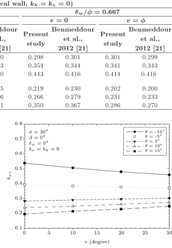
Table 2. ka for the associated and non-associated ow rules and their comparison with the numerical method of
Benmeddour et al. [21].
ka (vertical wall, kh= kv= 0)
w= = 0 w= = 0:667
v = 0 v = v = 0 v =
(degree) = Presentstudy
Benmeddour et al., 2012 [21]
Present study
Benmeddour et al., 2012 [21]
Present study
Benmeddour et al., 2012 [21]
Present study
Benmeddour et al., 2012 [21] 30 -0.333 0.4530 0.382 0.3610.411 0.3340.375 0.3300.373 0.2980.354 0.3010.344 0.3410.301 0.2990.343
-0.667 0.578 0.486 0.450 0.440 0.443 0.416 0.414 0.416
40 -0.333 0.4170 0.298 0.2810.327 0.2180.247 0.2150.246 0.2190.266 0.2300.279 0.2310.202 0.2000.233
-0.667 0.495 0.398 0.302 0.291 0.350 0.367 0.286 0.270
Figure 5. The eect of pseudo-static coecients on ka
( = 0).
results showed that ka is lower for associative soils
than that for the non-associative one. The maximum error between this study and the numerical method [21] is about 6% for the associated ow rule and 21% for the non-associated ow rule.
The variations of ka are also shown in Figure 6
( = 30) and Figure 7 ( = 20) for dierent values of
wall angle. The dierence due to a 10-degrees increase in dilation angle is almost 1.93-9.62% and 1.04-4.29% for = 30 (Figure 6) and = 20 (Figure 7),
respectively. Furthermore, the results of the analysis for dierent values of the ground slope are shown in Figures 8 and 9. The dierence is almost 0.42-4.62 and 1.09-4.59 percentages for = 30 (Figure 8) and
= 20 (Figure 9), respectively. The results showed
that the dilation angle eect on ka is low for = 30
and = 20. It is obvious that for associated ow
rule, kadecreases by increasing each of the soil friction
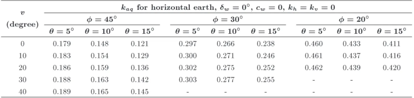
angle, wall angle, and the ground slope parameters. The dilation angle eect on kaq has been
consid-ered, as shown in Tables 3 and 4. kaq increases as
the dilation angle increases. The ranges of increase in kaq in Table 3 are 0.48-7.04, 0.27-3.36, and
0.15-Figure 6. The dilation angle eect on ka for dierent
values of wall angle in static case ( = 30).
Figure 7. The dilation angle eect on ka for dierent
values of wall angle in static case ( = 20).
1.39 percentages for soil friction angles equal to 40, 30, and 20 degrees, respectively. In Table 4, the kaq
increase ranges are 0.1-1.76, 0.13-1.61, and 0.15-1.65 percentages for soil friction angles equal to 40, 30, and 20 degrees, respectively. So, the dilation angle does not
Table 3. The eect of dilation angle on kaq for dierent values of wall angle.
v kaq for horizontal earth, w= 0, cw = 0, kh = kv = 0
(degree) = 45 = 30 = 20
= 5 = 10 = 15 = 5 = 10 = 15 = 5 = 10 = 15
0 0.179 0.148 0.121 0.297 0.266 0.238 0.460 0.433 0.411
10 0.183 0.154 0.129 0.300 0.271 0.246 0.461 0.437 0.416
20 0.186 0.159 0.136 0.302 0.275 0.252 0.462 0.439 0.420
30 0.188 0.163 0.142 0.303 0.277 0.255 - -
-40 0.189 0.165 0.145 - - -
-Table 4. The eect of dilation angle on kaqfor dierent values of ground slope.
v kaq for horizontal earth, w= 0, cw = 0, kh = kv = 0
(degree) = 40 = 30 = 20
= 5 = 10 = 15 = 5 = 10 = 15 = 5 = 10 = 15
0 0.207 0.197 0.187 0.315 0.300 0.285 0.462 0.439 0.419
10 0.208 0.199 0.190 0.317 0.303 0.290 0.464 0.443 0.426
20 0.208 0.200 0.193 0.318 0.304 0.293 0.464 0.445 0.430
30 0.209 0.201 0.195 0.318 0.305 0.294 - -
-40 0.209 0.202 0.195 - - -
-Figure 8. The dilation angle eect on ka for dierent
values of ground slope in static case ( = 30).
aect kaqconsiderably. But, its eect is clearer for the
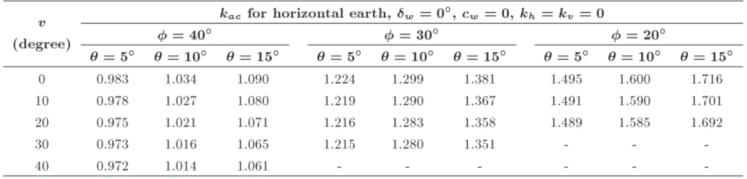
cases in which the wall angles are not equal to zero. Also, kac has been calculated for various values
of the dilation angle. The results have been shown in Tables 5 and 6. Obviously, increasing the dilation angle leads to decrease in kac. In the analysis for various
values of , the maximum decreases in kac are 0.92,
1.01 and 0.94 percentages and the minimum decreases are 0.3, 0.12 and 0.11 percentages for the soil friction angles equal to 20, 30, and 40 degrees, respectively. In the analysis for various values of , the maximum decreases of kac are 0.92, 1.02 and 0.94 percentages
and the minimum decreases are 0.13, 0.12 and 0.11 percentages for the soil friction angles equal to 20, 30,
Figure 9. The dilation angle eect on ka for dierent
values of ground slope in static case ( = 20).
and 40 degrees, respectively. So, the strongest eect of the dilation angle on kac is 1.01 percentage.
For associated ow rule, the eects of the soil friction angle, wall angle, and ground slope on kaq (see
Tables 3 and 4) and kac (see Tables 5 and 6) can also
be derived. kaq increases by decreasing each of the soil
friction angle, wall angle, and ground slope parameters. kac increases by decreasing the soil friction angle or
ground slope and increasing the wall angle.
The eect of dilation on the dynamic lateral earth pressure coecient, ka, has also been considered in
Figures 10 and 11 for = 40 and = 30,
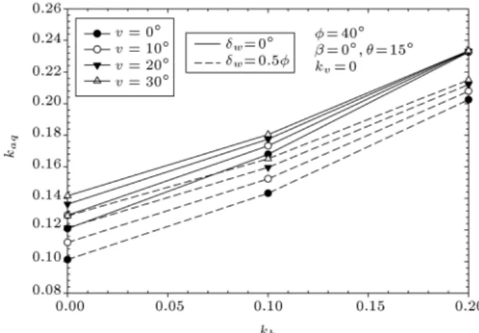
respectively. Similarly, Figures 12 and 13 have been provided for kaq. The least eect of dilation angle
Table 5. The eect of dilation angle on kac for dierent values of wall angle.
v kac for horizontal earth, w = 0, cw= 0, kh= kv= 0
(degree) = 40 = 30 = 20
= 5 = 10 = 15 = 5 = 10 = 15 = 5 = 10 = 15
0 0.983 1.034 1.090 1.224 1.299 1.381 1.495 1.600 1.716
10 0.978 1.027 1.080 1.219 1.290 1.367 1.491 1.590 1.701
20 0.975 1.021 1.071 1.216 1.283 1.358 1.489 1.585 1.692
30 0.973 1.016 1.065 1.215 1.280 1.351 - -
-40 0.972 1.014 1.061 - - -
-Table 6. The eect of dilation angle on kacfor dierent values of ground slope.
v kac for vertical wall, w = 0, cw= 0, kh = kv = 0
(degree) = 40 = 30 = 20
= 15 = 10 = 5 = 15 = 10 = 5 = 15 = 10 = 5
0 1.053 1.019 0.979 1.334 1.279 1.219 1.658 1.576 1.490
10 1.043 1.011 0.975 1.321 1.270 1.215 1.643 1.566 1.485
20 1.035 1.005 0.971 1.311 1.264 1.212 1.634 1.561 1.483
30 1.029 1.001 0.969 1.305 1.260 1.210 - -
-40 1.025 0.998 0.968 - - -
-Figure 10. The dilation angle eect on ka in dynamic
case ( = 40).
is observed for kh equal to 0.2. In this case, the
ka increase ranges from 0.26 to 0.94 percentages for
the smooth wall and from 0.54 to 5.95 percentages for the rough wall. Also, the kaq increase changes
from 0.09 to 2.38% for smooth wall, and from 0.14 to 2.6% for rough wall. The maximum increases of ka and kaq are observed for = 40 and kh = 0 by
increasing the dilation angle from zero to 10 degrees. The results showed that this maximum increase of ka
is 19.34% and 28.7% for the smooth and rough wall, respectively. Furthermore, this maximum increase of kaq is 6.57% and 9.72% for the smooth and rough
wall, respectively. It is clear that the dilation an-gle aects ka more than kaq and the lateral earth
Figure 11. The dilation angle eect on ka in dynamic
case ( = 30).
pressure coecients for the rough wall are more than the lateral earth pressure coecients for the smooth wall.
The dilation angle also aects the failure zone of the retaining wall. Figures 14 and 15 show the eect of the dilation angle on the failure surface for the smooth wall for = 40 and 30, respectively. Also,
Figures 16 and 17 have been prepared for the rough wall (w = ). As shown, the extent of the failure
zone decreases as the dilation angle increases. The dilation eect is the strongest for soil with the internal friction angle equal to 40 degrees. In this case, the extent of failure zone (at the ground surface) decreases from 3 to 1.40 meters for smooth wall (w = 0) and
Figure 12. The dilation angle eect on kaq in dynamic
case ( = 40).
Figure 13. The dilation angle eect on kaq in dynamic
case ( = 30).
Figure 14. The dilation angle eect on the failure zone ( = 40,
w= 0).
from 3.48 to 1.59 meters for rough wall (w = ).
Considering the dilation eect on the failure zone shows that the dilation angle aects the failure zone considerably and is more eective for rough retaining walls. The Monobe-Okabe (M-O) failure surfaces [24]
Figure 15. The dilation angle eect on the failure zone ( = 30,
w= 0).
Figure 16. The dilation angle eect on the failure zone ( = 40,
w= ).
Figure 17. The dilation angle eect on the failure zone ( = 30,
w= ).
are also shown in the Figures 14-17. As shown, for smooth walls, the M-O and associated ZEL failure surfaces are the same; but for rough walls, the failure surfaces are not linear and the M-O and associated ZEL failure surfaces are somewhat dierent.
4. Conclusions
In order to evaluate the lateral earth pressure on the retaining walls, the static and seismic lateral earth pressure coecients have been calculated using the method of zero extension lines. The results of the lateral earth pressure coecients due to the soil unit weight, surcharge, and soil cohesion are presented for associated and non-associated ow rules. The lateral earth pressure coecients were found to be compatible with other methods. A low dierence between ZEL method and other methods is observed and the dier-ence is equal to zero in many cases. The inudier-ence of the dierent parameters on the lateral earth pressure coecients has been explored.
For associative soils, ka and kaq decrease by
increasing each of the soil friction angle, wall angle, and ground slope parameters, and ka decreases by
increasing the soil-wall interface friction angle. Also, increasing the soil friction angle and ground slope and decreasing the wall angle decrease kac. The seismic
lateral earth pressure coecient kafor associative soils
increases as the horizontal and vertical pseudo-static coecients increase.
For non-associative soils, the dilation angle aects the lateral earth pressure coecients, slightly. By increasing the dilation angle, ka increases for plus
values of the wall angle and ground slope, and decreases for minus values of the wall angle and ground slope; kac decreases and kaq increases. The dilation angle
eect on the failure zone of the retaining wall is such that the extent of the failure zone in active case decreases considerably as the dilation angle increases. The dilation angle eects on ka, kaq, and the failure
zone of the retaining wall for the rough wall are more than those for the smooth wall.
Nomenclature q Surcharge Ground slope Wall angle
H Height of the retaining wall c Cohesion of the soil
Friction angle of the soil Unit weight of the soil v Dilation angle of the soil
w Friction angle of the soil-wall interface
cw Adhesion of the soil-wall interface
0 Normal stress on the ground surface
0 Shear stress on the ground surface
f Normal stress on the wall
f Shear stress on the wall
p Average stress
Angle between 1 and the horizontal
axis
p0 Average stress on the ground surface 0 The angle on the ground surface
pf Average stress on the wall f The angle on the wall
fx; fz Body forces along x and z directions
kh; kv Horizontal and vertical pseudo-static
earthquake coecients
d"+; d" Lengths of plus and minus zero
extension lines
ka Lateral earth pressure coecient due
to the unit weight of the soil
kaq Lateral earth pressure coecient due
to the surcharge
kac Lateral earth pressure coecient due
to the cohesion of the soil
References
1. Peng, M. and Chen, J. \Slip-line solution to ac-tive earth pressure on retaining walls", Geotechnique, 63(12), pp. 1008-1019 (2013).
2. Sokolovskii, V., Statics of Soil Media, Scienc. Publ., Butterworth, London (1960).
3. Askari, F., Totonchi, A. and Farzaneh, O. \Application of admissible stress elds for computation of passive seismic force in retaining walls", Sci. Iran, 19(4), pp. 967-973 (2012).
4. Chen, W. and Liu, X. \Limit analysis in soil me-chanics", Developments in Geotechnical Engineering (1990).
5. Iskander, M., Chen, Z., Omidvar, M., Guzman, I. and Elsherif, O. \Active static and seismic earth pressure for c soils", Soils Found., 53(5), pp. 639-652 (2013). 6. Lin, Y.L., Leng, W.M., Yang, G.L., Zhao, L.H., Li, L. and Yang, J.S. \Seismic active earth pressure of cohesive-frictional soil on retaining wall based on a slice analysis method", Soil Dyn. Earthquake Eng., 70, pp. 133-147 (2015).
7. Roscoe, K.H. \The inuence of strains in soil mechan-ics", Geotechnique, 20(2), pp. 129-170 (1970). 8. James, R. and Bransby, P. \A velocity eld for some
passive earth pressure problems", Geotechnique, 21(1), pp. 61-83 (1971).
9. Habibagahi, K. and Ghahramani, A. \Zero extension line theory of earth pressure", J. Geotech. Eng. Div., 105(7), pp. 881-896 (1979).
10. Anvar, S. and Ghahramani, A. \Equilibrium equations on zero extension lines and its application to soil
engineering", Iran J. Sci. Technol., 21(1), pp. 11-34 (1997).
11. Jahanandish, M. \Development of a zero extension line method for axially symmetric problems in soil mechanics", Sci. Iran, 10(2), pp. 203-210, Elsevier (2003).
12. Jahanandish, M. and Keshavarz, A. \Evaluation of static and dynamic stability of slopes by the zero extension line method", in Fourth International Con-ference of Earthquake Engineering and Seismology, SEE4, Tehran, Iran (2003).
13. Jahanandish, M., Mansourzadeh, S. and Emad, K. \Zero extension line method for three-dimensional stability analysis in soil engineering", Iran J. Sci. Technol. B, 34(B1), pp. 63-80 (2010).
14. Jahanandish, M., Veiskarami, M. and Ghahramani, A. \Investigation of foundations behavior by implementa-tion of a developed constitutive soil model in the ZEL method", Int. J. Civ. Eng., 9(4), pp. 293-306 (2011). 15. Behpoor, L. and Ghahramani, A. \Zero extension line
theory of static and dynamic bearing capacity", in Frac, Huft Asian Regional Conference on Soil Mechan-ics and Foundation Engineering (1987).
16. Behpoor, L. and Ghahramani, A. \Recommendation for evaluation of dynamic earth pressure on retaining structures for Iranian earthquake code", in Second International Seminar on Soil Mechanics and Foun-dation Engineering of Iran, Shiraz University, Iran (1993).
17. Behpoor, L. and Ghahramani, A. \Undrained bearing capacity of clay by zero extension line", in Proceedings of the International Conference on Soil Mechanics and Foundation Engineering - International Society for Soil Mechanics and Foundation Engineering, A.A. Balkema (1994).
18. Veiskarami, M., Jahanandish, M. and Ghahramani, A. \Prediction of foundations behaviors by a stress level based hyperbolic soil model and the ZEL method", Computational Methods in Civil Engineering, 1(1), pp. 37-54 (2010).
19. Veiskarami, M., Jahanandish, M. and Ghahramani, A. \Application of the ZEL method in the prediction of foundation bearing capacity considering the stress level eect", Soil Mech. Found. Eng., 47(3), pp. 75-85 (2010).
20. Veiskarami, M., Jahanandish, M. and Ghahramani, A. \Prediction of the bearing capacity and load-displacement behavior of shallow foundations by the stress-level-based ZEL method", Sci. Iran, 18(1), pp. 16-27 (2011).
21. Benmeddour, D., Mellas, M., Frank, R. and Mabrouki, A. \Numerical study of passive and active earth pressures of sands", Comput. Geotech., 40, pp. 34-44 (2012).
22. Lee, I. and Herington, J. \A theoretical study of the
pressures acting on a rigid wall by a sloping earth or rock ll", Geotechnique, 22(1), pp. 1-26 (1972). 23. Shiau, J. and Smith, C. \Numerical analysis of passive
earth pressures with interfaces", in Proceedings of the III European Conference on Computational Mechanics (ECCM 2006), Springer-Verlag (2006).
24. Kramer, S.L., Geotechnical Earthquake Engineering, Prentice Hall, New Jersey (1996).
Appendix
The parameters in Eqs. (14)-(17) are:
tgmp = tan( C+ C) + tan( 2 B+ B); (A.1)
tgmm = tan( C C) + tan( A A)
2 ; (A.2)
A3= pB pA+ A1+ BBmp Bmm A A2;
(A.3) A4= Bmp Bmm; (A.4)
where: Bmp=
+ BCAC
[(pC+ pB) tan + 2c] ; (A.5)
A1= Cmp+ Dmp; (A.6)
Cmp= fx[(xC xB) (zC zB) tan ] ; (A.7)
Dmp= fz[(xC xB) tan + (zC zB)] ; (A.8)
Bmm=
+ ACBC
[(pC+ pA) tan + 2c] ;
(A.9) A2= Cmm+ Dmm; (A.10)
Cmm= fx[(xC xA) (zC zA) tan ] ; (A.11)
Dmm= fz[ (xC xA) tan + (zC zA)] :
(A.12)
Biographies
Amin Keshavarz is currently an Assistant Professor of Civil Engineering in the School of Engineering at Persian Gulf University, Iran. He received his BSc degree in Civil Engineering from Persian Gulf University in 1997. He also received his MSc and PhD degrees in Civil Engineering (Soil Mechanics and Foundations) from Shiraz University, Iran, in 2000 and 2007, respectively. His research interests are stress characteristics and ZEL methods, soil dynamics and geotechnical earthquake engineering, and stability
analysis of reinforced and unreinforced soil slopes and retaining walls.
Zahra Pooresmaeil received her BSc degree in Civil Engineering from Persian Gulf University, Iran, in 2011. She was accepted for MSc degree in 2012. Her
eld of study was Soil Mechanics and Foundations. In 2014, she attended the 2nd Iranian Conference on Geotechnical Engineering and the 8th National Congress on Civil Engineering and presented some parts of her thesis. She received her MSc degree from Persian Gulf University in 2014.
![Figure 2. The directions of zero extension lines and Mohr circle of the strain [10].](https://thumb-us.123doks.com/thumbv2/123dok_us/8383725.2227522/4.892.166.752.156.416/figure-directions-zero-extension-lines-mohr-circle-strain.webp)