Comprehensive Simulation of Surface
Texture for an End-Milling Process
B.M. Imani
and E. Layegh
1The analysis and simulation of the manufacturing process require extensive and complicated computations. Nowadays, computer resources and computational algorithms have reached the stage where they can model and simulate the problem eciently. One of the important processes in manufacturing is machining. In this research, the end-milling process, which is one of the most complex and widespread processes in machining, is chosen. The most important parameters in end-milling are surface roughness and surface location errors. Comprehensive simulation software is developed to model the end-milling process, in order to anticipate the nishing parameters, such as surface roughness and errors. The proposed algorithm takes into account cutting conditions, such as feed, doc, woc and tool run out etc. In addition, the dynamic simulation module of the software can accurately model the exible end-mill tool, the milling cutting forces and regeneration of the waviness eects, in order to construct a realistic surface texture model. The software can accurately determine the most commonly used index of surface roughness parameters, such as Ra, P.T.V. and surface errors.
INTRODUCTION
End-milling operations are extensively used in the production of precise parts in industry. Milling process dynamics have been investigated in much research work. However, due to the complexity of the process, dierent elds of research are required. One area in the analysis and simulation of the milling process is in the developing of a comprehensive model, in order to anticipate surface quality, dimensional error and their trends in mass production. In various machining processes, the following steps are required to build up the model:
1. Analysis and modeling of the machining forces, 2. Modeling of the dynamic system of machine tools, 3. Modeling of the surface texture.
A comprehensive model for the accurate anticipa-tion of surface errors requires a \precise" force model. The model must take account of phenomena such as, tool deections, tool run-out, tool wear and machining
*. Corresponding Author, Department of Mechanical En-gineering, Ferdowsi University of Mashhad, I.R. Iran. E-mail: [email protected]
1. Department of Mechanical Engineering, Ferdowsi Uni-versity, Mashhad, I.R. Iran.
dynamics etc. In the most ofprevious research work, machining forces are obtained by using a mechanistic force model based on oblique cutting tests [1]. In this work, the orthogonal cutting theory and transforming method proposed by E. Budak et al. is used [2]. In contrast to previous methods, there is no need for an oblique cutting test for each tool shape. At rst, a gen-eral machining database is provided using orthogonal cutting tests with various work materials and cutting tool materials. Using transforming relations and tool geometry, the cutting coecients for oblique cutting are determined.
In general, one of the important sources of vibra-tion in the milling process is the self-excited vibravibra-tion. In this kind of vibration, internal sources will provide energy for the system. In some cases, the energy will exceed damping, thus vibrations sustain or even grow in amplitude. One of the important principles observed in machining dynamics is the regeneration of waviness, which aects chip thickness [3].
In the current research, a dynamic simulation model for machining dynamics is proposed. The surface is modeled using a 3D algorithm, which is an extension to available 2D methods [4]. The devel-oped simulation model can anticipate surface rough-ness in any direction of interest on the machined surface.
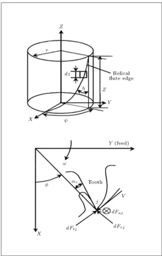
SIMULATION OF CUTTING FORCES Figures 1a and 1b illustrate the coordinate system and the end-milling geometry required for the model. Dierential forces, dft tangential, dfr radial and dfa
axial are depicted, which act on the jth cutting edge for an ideal system (without any deection). Values of the dierential forces are obtained by the following (for tooth j):
dftj(; z) = [Kte+ Ktchj(; z)]dz;
dfrj(; z) = [Kre+ Krchj(; z)]dz;
dfaj(; z) = [Kae+ Kachj(; z)]dz: (1)
In Equations 1 there are two separate terms, the rst one is related to friction and ploughing forces and the second term is considered for the cutting action that takes place in the shear zone. Coecients for the rst phenomena are represented by Kte, Kre, and Kae,
showing the amount of force per unit length of the cutting edge. Coecients represented by Ktc, Krc and
Kacare considered for the cutting action, showing the
amount of force per unit area of cutting edge.
Figure 1. Coordinate system and end-milling geometry.
The simulation software, written in MATLAB V7.0, rst computes cutting and edge force coecients and then computes the cutting forces for each cutter angle [5]. Table 1 summarizes the computed coecients for a four-ute HSS tool and the aluminium work-piece, 7075-T6, with a yield stress of 542 MPa. The computed cutting forces are depicted in Figure 2.
REGENERATION OF WAVINESS
In general, the cutting edge of the tool is cutting a surface, which has been generated in the previous passes. If any vibrations exist between the tool and the work piece, the newly generated surface undulates, which results in the variation of chip thickness. Fig-ure 3 illustrates the model used for the simulation of the milling process. The dynamic characteristics of the system in x and y directions are also depicted. Dierential forces can be obtained by the following:
dFtn+1 = Ktcda(h0 zn+ zold1+ zold2+ zold3);
dFrn+1 = Krcda(h0 zn+ zold1+ zold2+ zold3): (2)
Table 1. The computed coecients for a four-ute HSS tool and an aluminium work-piece, 7075-T6, with a yield stress of 542 MPa. In this table, nis the normal rake
angle of the tool. n
(deg)
Ktc
[N/mm2]
Krc
[N/mm2]
Kac
[N/mm2]
0 1642.3 609.5 512.2 12 1396.2 519.8 258.1 15 1356.5 504.4 215.3
Figure 2. Simulated cutting forces for a four-ute HSS tool and an aluminium work-piece, 7075-T6, with yield stress of 542 MPa. Cutting conditions are d (tool
diameter) = 10 mm, ft (feed per tooth) = 0.05 mm/tooth,
Figure 3. Model used for simulation of the dynamic milling process.
Due to the fact that the axial stiness of the tool and the spindle assembly is high and also that the axial force is smaller than the others, the axial vibrations are ignored. In the above relations, n, h0, zn, zold1 to
zold3and da are, respectively, index of time increment,
nominal chip thickness, tool deection normal to the cut surface, tool deection in previous passes and axial increment. In each instance, the dierential cutting forces on the engaged cutting edges are computed and projected on an X and Y axis. Then, the total cutting forces are computed by integration of the dierential forces over the engaged edges. Using Newton's second law, dierential equations of motion are written and, then, using double Euler integration, the dynamic deections are obtained as follows.
Fxn+1 = mxxn+ Cx_xn+ Kxxn;
Fyn+1 = myyn+ Cy_yn+ Kyyn; (3)
where mx, my, Kx, Ky, Cx and Cy are mass, stiness
and damping matrices for x and y directions, respec-tively. Input data for a four-ute end-mill with a helix angle of 30 are considered as follows [6,7]:
fx= fy= 660 HZ; Kx= Ky= 2 107N/m;
Mx= Kx=(2fx); My = Ky=(2fy);
x= y= 0:05; Cx= x 2
p KxMx;
Cy = y 2
p
KyMy; r = 5 mm;
n = 1200 rpm; doc = 10 mm: (4)
In the above relations, fx, fy, xand yare the natural
frequency and damping ratios for x and y directions, respectively. The tool radius, spindle speed and depth of cut are represented by r, n and doc. The nominal chip thickness at angular position is:
h0= ft sin : (5)
Normal to cut deection is:
Zn= xnsin + yncos : (6)
Using the proposed model, it is possible to include non-linearities, such as jump-of-cut and chatter vibrations. Figure 4 shows the simulation results for an aluminium 7075-T6 work piece. Cutting conditions are d = 10 mm, h (helix angle) = 30, ft = 0:1 mm/tooth, woc
(width of cut) = 1.2 mm, n = 1200 rpm, doc (depth of cut) = 10 mm.
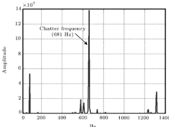
Dynamic milling forces for woc = 3 mm are shown in Figure 5. The Fourier transform of the
Figure 4. Dynamic simulation of cutting forces for aluminium 7075-T6 work piece. Cutting conditions are d = 10 mm, h = 30, ft = 0:1 mm/tooth, woc = 1:2.
Figure 5. Dynamic simulation of cutting forces for aluminium 7075-T6 work piece. Cutting conditions are d = 10 mm, h = 30, ft = 0:1 mm/tooth, woc = 3 mm.
milling forces are computed and depicted in Figures 6 and 7. Tooth passing is the dominant frequency in stable cutting. However, as inferred from Figures 6 and 7, the dominant frequency in unstable cutting is close to the natural frequency of the exible mode shape, known as chatter frequency [6]. When woc = 3 mm, milling is unstable and the vibration grows in amplitude gradually.
DYNAMIC VIBRATIONS OF TOOL AND SPINDLE
Surface roughness prediction requires a comprehensive model in the time domain, which can simulate tool vibrations at locations of interest on the work piece. In the current research, milling vibrations are modeled by FEM using the CALFEM toolbox implemented in MATLABV7.0 software [8].
Figure 8 schematically shows the FEM model for the end-mill and spindle assembly, which is modeled as a step beam with two simple supports.
Figure 6. Fourier transform for Fx.
Figure 7. Fourier transform for Fy.
Figure 8. FEM model for the end-mill and spindle assembly.
The axial variation of the tool deection is com-puted for the engaged portion of the tool, which is used by the surface location error algorithm. Therefore, ner elements in this portion are introduced.
Inputs for FE analysis are given in the follow-ing [9]:
modulus of elasticity of steel = 207 109 (N/m2),
inner diameter of spindle axis = 0.02 m, outer diameter of spindle axis = 0.1 m, density of steel = 7800 (Kg/m3).
Figure 9 illustrates the developed owchart of the FE analysis.
In the developed algorithm, Nr, a, da, F0, T (N),
X(N; j) and Y (N; j) are number of revolutions, axial depth of cut, axial increment, initial force, time and x-and y-deections, respectively. Inputs to the algorithm are tool radius, woc, doc, feed, cutting force constants and spindle speed. A function written in MATLAB V7.0 is used to calculate mass, stiness and damping matrices. Using mesh and node positions, the mass, stiness and damping of each element are computed and then assembled together to get overall matrices. In addition, boundary conditions and external cutting forces are applied. Dierential equations of motion are integrated numerically by the Newmark method.
(
MxX + C xX + K_ xX = FX
MyY + C y_Y + KyY = FY (7)
For selected initial values of y = x = _y = _x = 0, the initial acceleration is expressed as follows:
X = F CMx_x kxx
x ;
Y = F CMy_y kyy
y : (8)
The iteration loop starts from 1 and ends at a=da (where a is DOC and da is axial increment). Thus, the variation in axial deection is obtained. Counter
Figure 9. Developed owchart of the FEM analysis.
N varies from 1 to Nr 1, which is considered for the time increments. After computing Fx, Fy, x, and y
at current time increments, these values are used as initial values for the next step. Results of the milling tool in the time domain by FE analysis are shown in Figure 10. Vibrations of the tool center point are plotted at dierent axial levels.
In the next section, the amount of vibration is used for determining the cutting edge position and the surface generation method.
TOOL PATH SIMULATION
The nal machined surface is produced by subsequent cutting actions of end-mill cutting edges. Ideally, points on the cutting edge have trochoidal paths, which leave feed marks on the surface. Additionally, any tool deection, vibration or geometric error results in
Figure 10. Results of time domain FE analysis of the milling tool for d = 12 mm, ft= 0:3 mm/tooth,
Ktc= 2000 N/mm2, doc = 5 mm, woc = 1:5 mm.
undesirable deformation and deteriorates the required surface roughness on the work piece. The ideal position of the cutting edges, with respect to the tool cutter, is shown in Figure 11.
The XOY coordinate system is attached to the work piece and the original O is at the initial center position of the spindle. The trochoidal motion of a point on the cutting edge is computed by [9]:
Xl=c(i; z; t) = R sin((t) (i) (z));
Yl=c(i; z; t) = R cos((t) (i) (z)); (9)
where Xl=c and Yl=c are coordinates of the edge, with
respect to the tool center point. Also, i, r, (t), (i) and (Z) are tooth index, tool radius, angular position
Figure 11. Trochoidal path of a point on the cutting edge.
of the lowest point of the reference cutting edge, pitch angle and phase lag of the point at z levels, respectively.
(Z) is computed by:
(Z) = z tanhR ; (10)
where h is tool helix angle.
On the other hand, displacement of the spindle center, with respect to the work piece, can be found by:
Xs=w = fr (t)=(2);
Ys=w= 0: (11)
If the runout error is not negligible, the location of the tool center, with respect to the spindle axis, will be computed by:
Yc=s(t; z) = cos((t) + ) + YFEM(t; z);
Xc=s(t; z) = sin((t) + ) + XFEM(t; z); (12)
where is runout oset and is its angular position (refer to Figure 12).
XFEM(t; z) and YFEM(t; z) are the dynamic tool
deections at time t and z level, which are calculated by FE analysis. Thus, instantaneous positions of a point on the cutting edge can be found by:
Xl=w= Xl=c+ Xc=s+ Xs=w;
Yl=w= Yl=c+ Yc=s+ Ys=w: (13)
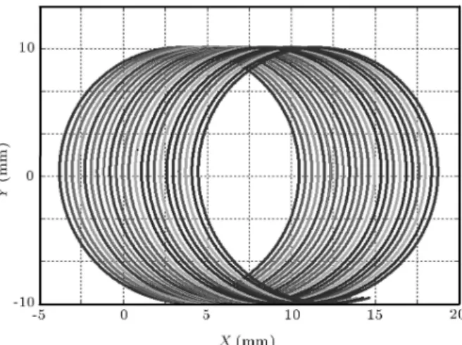
Figure 13 shows the trochoidal motion of the cutting edges without considering vibrations and runout. In order to show the eects of the runout, its value is set to 1 mm, which is exaggerated intentionally. The other cutting conditions are kept constant. The simulation results are shown in Figure 14. Finally, Figure 15
Figure 12. Runout parameters.
Figure 13. Trochoidal motions of the cutting edges without considering vibrations and runout (ft= 1
mm/tooth, d = 20 mm).
Figure 14. Trochoidal motions of the cutting edges with considering exaggerated runout ( = 1 mm, = 45).
shows the path of the cutting edge, including tool vibrations.
SURFACE TEXTURE SIMULATION
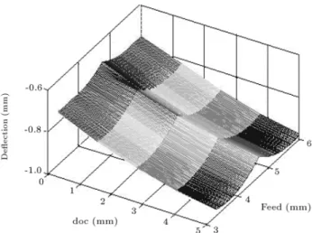
Feed mark proles can be produced by removing the points on the computed paths, which do not make contact with the newly generated surface. The z-level proles are used in the mesh function to construct a 3D surface. Figures 16 to 18 illustrate 3D mesh surfaces for dierent cutting conditions. The cutting conditions used for the simulation of Figure 16, result in negligible vibrations. In order to show the runout eects, an exaggerated runout oset ( = 1 mm) is chosen and the result of the simulation is shown in Figure 17. Extreme cutting conditions, which result in chatter vibrations, are used for the simulation of Figure 18.
As shown in Figures 10 and 18, the amplitude of the vibrations at the tool tip is much higher. Table 2
Figure 15. Trochoidal motions of the cutting edges with considering vibrations (d = 12 mm, ft= 0:3 mm/tooth).
Figure 16. Surface texture for d = 12 mm, woc = 1 mm, doc = 5 mm, ft= 0:1 mm/tooth, Ktc= 1500 N/mm2 (Ra
= 1.4 ).
Figure 17. Surface texture for d = 10 mm, woc = 1 mm, doc = 5 mm, ft= 0:1 mm/tooth, Ktc= 1500 N/mm2,
= 1 mm (Ra = 3.5 ).
Figure 18. Surface texture for d = 12 mm, woc = 4:5 mm, doc = 5 mm, ft= 0:6 mm/tooth, Ktc= 1500
N/mm2, = 0:01 mm (Ra = 14 ).
Table 2. Surface roughness computed at tool tip. d
(mm) a (mm)
W OC (mm)
ft (mm/tooth)
Ra 10 5 1.0 0.05 1.14 10 5 1.5 0.1 3.99 10 5 1.5 0.25 5.85 12 5 1.5 0.1 2.24 12 5 2 0.1 3.07 12 5 3 0.15 4.61
summarizes the Ra values of the surface roughness computed at the tool tip.
CONCLUSIONS
In this research work, a comprehensive simulation model is developed for anticipating dynamic cutting forces and 3D surface texture for end-milling opera-tions. The variation of instantaneous tool deections are computed by FE analysis, using the CALFEM toolbox implemented in the MATLAB V7.0 environ-ment. Variations of dynamic tool deections are also computed along the axial direction for constructing the 3D surface texture model. The nal model contains all the information required to compute the surface roughness parameter and surface location errors. REFERENCES
1. Budak, E. and Altintas, Y. \Flexible milling force model for surface error prediction", Proceeding of the Engineering System Design and Analysis, Istanbul, Turkey, pp 89-94 (1992).
2. Budak, E., Altintas, Y. and Armarego, E.J.A., Pre-diction of Milling Force Coecient from Orthogonal
Cutting Data, 1st Ed., Cambridge University Press, NY, USA (1996).
3. Smith, S. and Tlusty, J. \An overview of modelling and simulation of milling process", ASME Journal of Engineering for Industry, 113(2), pp 169-175 (1991). 4. Yun, W.S., Ko, J.H., Cho, D.W. and Ehman, K.
\Development of a virtual machining system. Part 2: Prediction and analysis of a machined surface error", International Journal of Machine Tools & Manufac-turing, 42, pp 1607-1615 (2002).
5. MATLAB V7.0, MathWorks, Inc, www.mathworks. com .
6. Altintas, Y., Manufacturing Automation, Metal Cut-ting Mechanics, Machine Tool Vibration and CNC Design, Cambridge University Press (2000).
7. Tlusty, J., Manufacturing Process and Equipment, Prentice Hall, New Jersey (2000).
8. CALFEM, a Finite Element Toolbox, V3.3, LUND University, Sweden.
9. Montgomery, D. and Altintas, Y. \Mechanism of cut-ting force and surface generation in dynamic milling", ASME Journal of Engineering for Industry, 113, pp 160-168 (1991).