Sharif University of Technology
Scientia IranicaTransactions B: Mechanical Engineering www.scientiairanica.com
Parameter identication of a parametrically excited
rate micro-gyroscope using recursive least squares
method
Z. Mohammadi and H. Salarieh
School of Mechanical Engineering, Sharif University of Technology, Tehran, Iran.
Received 7 September 2014; received in revised form 4 September 2015; accepted 5 September 2016
KEYWORDS Gyroscope;
Parametric excitation; Estimation;
Physical parameters; Least squares method.
Abstract. Estimation of physical parameters of a parametrically excited gyroscope is studied in this paper. This estimation is possible by reading the input and output data of the gyroscope. Because of dierent faults in the manufacturing process and tolerances, physical parameters of a gyroscope are not exactly same as the expected values of the manufacturer. Moreover, changing of temperature, humidity, external acceleration, etc. can change the physical parameters of the gyro. Thus, the physical parameters of gyroscope are not xed values and may deviate from the desired designed values. The physical parameters of gyroscope determine the optimal region for working of gyroscope. Thus, if the parameters deviate from the original ones but the excitation frequency is xed at its initial value, the sensitivity of the gyroscope will be reduced. The new parameters of the gyroscope can determine the new point of excitation frequency and, because of this, estimation of these parameters should be done to prevent sensitivity reduction. Estimation of these new parameters using the input and output values is studied here.
© 2017 Sharif University of Technology. All rights reserved.
1. Introduction
Estimating of parameters of a parametrically excited gyroscope using the least squares method is investi-gated in this paper. This estimation will be done by measuring the input and output signals of the gyro. The new point for optimum working of gyroscope is calculated with new estimated parameters. The excitation frequency will be calculated using these parameters, too.
Rate gyros measure the body angular velocity of the devices on which they are installed. Among dierent types of gyros, MEMS gyros are in focus, because of low cost and low energy consumption [1].
*. Corresponding author. Tel.: +98 21 6616 5538; Fax: +98 21 6600 0021
E-mail address: [email protected] (H. Salarieh)
MEMS gyros are mainly used in vehicle industries; nav-igation systems of airplanes, especially low-cost drones; stability control of cars; robotics; biomechanics; and rollover detection of vehicles [1-6]. Dierent types of MEMS gyros are tuning fork [1,3,7-10], proof mass [1], and ring gyroscopes [1,3,10]. In this paper, proof mass MEMS gyros are investigated because of their simple conguration and wide use [6,11,12]. Proof mass is driven in the drive direction (x axis) using electrostatic harmonic force that is generated using some comb-nger electrodes with dierent voltages. Existing angular velocity in the z direction creates a motion in the y axis (sense direction) because of Coriolis eects. The angular velocity is determined measuring the amplitude of the sense direction. The more is the angular velocity, the more is the sense direction's amplitude [3]. These gyroscopes are called harmonic drive gyros.
Coriolis force creates movement in the sense di-rection; the frequency of this force is equal to the drive frequency. Thus, maximum force and displacement in the sense direction and, consequently, maximum sensitivity are attained when, rst, the drive frequency is equal to the natural frequency in the drive direction and, second, the natural frequencies in the drive and sense directions are equal to each other. Because of this, small changes in natural frequency in each direction may signicantly reduce sensitivity of the gyroscope. This change can happen because of manu-facturing errors or change in temperature, humidity, or environmental conditions.
Many researchers, like Alper et al., have tried to modify manufacturing errors for improving the robust-ness of the gyroscope when changing environmental conditions [6,11-13].
Other methods, like closed loop control methods, make resonances in the drive mode only or in the drive and sense modes. Yi et al. made resonance in the drive mode for amplitude and phase control using a PI controller and some electronic circuits [14]. Chang et al. in [15] made resonances in drive and sense modes with phase dierence control method. In [16], forced control algorithms based on adaptive control methods are presented for making resonances in the drive and sense modes.
Another method for solving the problems of har-monic excitation in MEMS gyroscopes is parametric excitation. Physical structure of these gyros is similar to that of the harmonic excitation gyroscopes. The dierence is in the drive mode electrodes' congu-ration that changes the system's equations. In this method of excitation, mismatching between the natural frequencies of the drive and sense modes does not reduce the gyroscope's sensitivity to the extent that it does in the harmonically excited gyros. This is because of large bandwidth of the drive mode; thus, natural frequency of the sense mode can be in any point of the frequency bandwidth of the drive mode. Therefore, because of larger bandwidth of the drive mode of a parametrically excited gyro, if the natural frequency of each mode changes due to environmental conditions or tolerance errors, its sensitivity will not be reduced signicantly. Compared with manufacturing modication methods, parametric excitation needs low cost and time. Control methods need some electronic devices and circuits such as controller; this leads to increased cost in comparison with parametric excita-tion method that needs only some modicaexcita-tions in electrodes conguration. This idea was rst pub-lished by Oropeza-Ramos in 2005 and the result was shown with numerical simulation [17]. After that, in [5,18], the operating specications of a parametri-cally excited gyroscope were reported. In Pakniyat's works [19,20] some parametric study and stability
analysis for dierent parameters of the gyroscope were done.
Here, the suspension system of the gyroscope is assumed to be like that in Alper and Akin's work [6,11,12].
As mentioned in [19,20], the optimum drive fre-quency for parametrically excited gyroscope is twice the natural frequency of the sense mode. This will be shown in the following sections. Thus, knowing the gyroscope's parameters is needed for maximizing its output amplitude.
In this paper, the parameters of a parametrically excited gyroscope will be estimated. The proposed method can be used in a gyroscope to nd the op-timal point for its working with maximal sensitivity and estimating the external angular velocity, which is a completely novel method of measurement. For estimating the parameters of the system, the equations of the system are modied. The external acceleration terms, coupling stiness, and damping are considered in the equations, too. These terms are estimated as well as the physical terms of the gyro.
In Section 2, the dynamical equations of paramet-rically excited gyros will be determined and, then, the equation will become dimensionless using the dened parameters. In Section 3, the least squares estimator will be explained. In Section 4, simulation results that show the correct estimation of parameters will be shown, and Section 5 contains the conclusion of this work.
2. Determining the dynamical equations of gyroscope
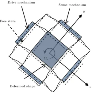
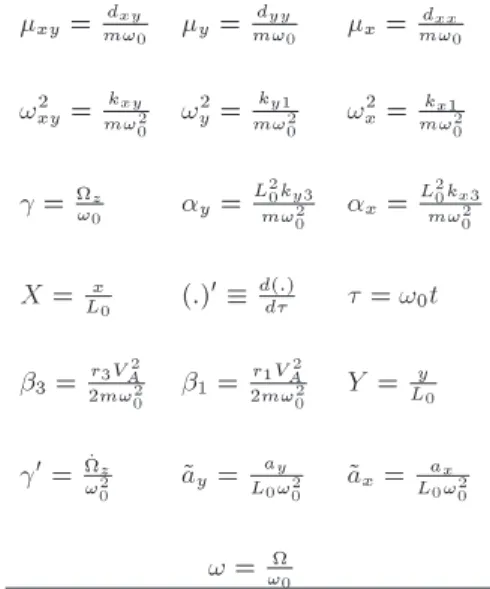
The structure of the gyroscope is similar to the pre-sented gyro in [6,11,12] as was mentioned before. A scheme of this gyroscope is shown in Figure 1 and structural model of the gyroscope is shown in Figure 2. The drive electrodes are similar to the shown
g-Figure 1. Schematics of the designed gyroscope in [6,11,12] and in this paper.
Figure 2. Structural model of the gyroscope in this paper. Dashed line: free state, and solid line: deformed shape.
Figure 3. The conguration of electrodes in harmonically excited gyroscope.
Figure 4. The conguration of electrodes in parametrically excited gyroscope.
ures in Figures 3 and 4, when the actuation mechanism is of harmonic or parametric type, respectively.
For determining the gyroscope's equation of mo-tion, the frame coordinate system is chosen in the center of gyro. Thus, the equations will be found as follows.
F = ma; F
m =a = ao+ arel+ !f (!f r) + _!f r + 2!f v !a = aox^i+ aoy^j + aoz^k + x^i+ y^j + z^k
+x^i+ y^j + z^k
x^i+ y^j + z^k
x^i + y^j + z^k+_x^i+ _y^j + _z^k
x^i + y^j + z^k+ 2x^i+ y^j + z^k
_x^i + _y^j + _z^k=
x + aox^i+ xyy
+ xzz 2yx 2zx + _yz _zy
+ 2y_z 2z_y
^i+y + aoy^j 2xy
+ xyx + zyz 2zy _xz + _zx
2 _x_z + 2z_x)
^j + biggl(z + aoz^k 2xz
2
yz + xzx + yzy + _x_y _y_x
+ 2x_y 2y_x
^k: (1)
In Eq. (1), ^I, ^J and ^k are the coordinate axes in body frame; F and a are the total force on the gy-roscope's proof mass and the proof mass' acceleration, respectively; m is the mass of the proof mass; ao is
the acceleration of the center of frame coordinate (aox,
aoy, and aoz in x, y, and z directions, respectively);
and arel is the relative acceleration of the lumped mass
center with respect to the frame coordinate system (x, y, and z in x, y, and z directions, respectively), both of them stated in the body coordinate system; !f is the
angular velocity of gyroscope frame stated in the body coordinate (x, y, and z in x, y, and z directions,
respectively) and r is the coordinate of any point of gyroscope relative to frame axes, both of them in body axes; _!f is the angular acceleration of gyroscope frame
( _x, _y, and _zin x, y, and z directions, respectively);
and v is the velocity of any point of gyroscope stated in body coordinate ( _x, _y, and _z in x, y, and z directions, respectively).
Total external forces on the vibrating body are written in Eq. (2):
Fi= Fia Fir Fid: (2)
Fa
i is the actuation force; Firis the restoring force; and
Fd
i is the damping force in the i direction (x, y, or z
direction).
Now, some assumptions will be applied for sim-plifying Eq. (1):
Actuating force is in the x direction only;
Angular velocity is in the z direction only. (x =
y = 0);
Displacement of the mass is constrained in the z direction (z = _z = z = 0);
Linear viscous damping exists in the system; Restoring force is of degree 3; force in each direction
is a function of displacement in that direction (Fr
i(xi) = k1xi+ k3x3i);
Coupling stiness and damping are the same in x and y directions (dxy= dyx, kxy= kyx);
Actuating force is of the following form [5,21]: Fa(x; t) = (r
1x + r3x3)[V (t)]2; (3)
V is voltage dierence between the electrodes of parametric excitation; r1 and r3are the parametric
excitation coecients that can be calculated ac-cording to electrode length and width, and their numbers, and the gap between them. The voltage dierence is as follows:
V (t) = VAp1 + cos 2t; (4)
where VA is the amplitude of voltage dierence and
is the frequency of this change.
Regarding the above assumptions, the nal equa-tions for working of the gyroscope are in the form of Eq. (5). 8 > > > > > > > > > > > < > > > > > > > > > > > :
mx + dxx_x + (kx1 m2z)x + kx3x3
+kxy m _z
y + (dxy 2mz) _y
+ r1xVA2(1 + cos 2t) + r3x3VA2(1 + cos 2t)
= max
my + dyy_y + ky1 m2z
y + ky3y3
+kxy+ m _z
x + (dxy+ 2mz) _x = may
(5)
The non-dimensional parameters will be dened in the form shown in Table 1, where xy, x, and y
are the non-dimensional cross damping in the drive direction and in the sense direction. The dimensional damping parameters are dxy, dx, and dy. !xy is
the non-dimensional cross natural frequency. !x and
!y are the non-dimensional natural frequencies of the
drive and sense modes, and ! is the non-dimensional excitation frequency. The linear stiness in the x and y directions is kx1 and ky1 and cross stiness is
kxy. x and y are the non-dimensional nonlinear
stiness. The nonlinear stiness is kx3 and ky3.
and 0 are the non-dimensional angular velocity and
Table 1. Denition of non-dimensional parameters and non-dimensional derivation.
xy= m!dxy0 y=m!dyy0 x=m!dxx0
!2 xy= m!kxy2
0 !
2 y=m!ky12
0 !
2 x= m!kx12
0
= z
!0 y=
L2 0ky3
m!2
0 x=
L2 0kx3
m!2 0
X = x
L0 (:)
0 d(:)
d = !0t
3= r3V
2 A
2m!2 0 1=
r1VA2
2m!2 0 Y =
y L0
0= _z
!2
0 ~ay=
ay
L0!20 ~ax=
ax
L0!20
! = !0
acceleration of the gyroscope. z is the external
angular velocity and _zis the external angular
acceler-ation. X and Y are the non-dimensional displacement (dimensional terms are \x" and \y") in the drive and sense directions and L0 is equal to 1 m. is
the non-dimensional time. 1 and 3 are the
non-dimensional electrostatic excitation terms, respectively. The electrostatic excitation terms are r1for linear and
r3 for nonlinear. ~ax and ~ay are the non-dimensional
linear accelerations in the drive and sense modes. The accelerations in the drive and sense modes are ax
and ay. !0 is the natural frequency of the drive
mode.
Except acceleration term in the right side of Eq. (5), some of the parameters in the left side of that equation are time-dependent. Because of this, time-dependent terms are transferred to the right side of the equation and considered as inputs. The non-dimensional equations are in the form of Eq. (6). 8 > > > > > > > > > > > > > > > > > > > < > > > > > > > > > > > > > > > > > > > :
X00+ xX0+
!2 x 2 z !2 0
X + xX3
+ !2 xy !_z2
0
! Y +
xy 2!z 0
Y0
+ 21X + 23X3= ~ax 21X cos 2!
23X3cos 2!
Y00+ yY0+
!2 y 2 z !2 0
Y + yY3
+ !2 xy+!_z2
0
! X +
xy+ 2!z 0
X0 = ~a
y:
(6)
Writing these equations in the state space form results in the following equations:
8 > > > > > > > > > > > > > > > > > > > > > > > > > > > > > < > > > > > > > > > > > > > > > > > > > > > > > > > > > > > :
_x1= x2
_x2= xx2+
!2
x 2 z
!2 0
x1
+ !2 xy !_z2
0
! x3+
xy 2!z 0
x4
+21x1+(23+x)x31+~ax 21x1cos 2!
23x31cos 2!
! _x3= x4
_x4= yx4+
!2
y 2 z
!2 0
x3+ yx33
+ !2 xy+!_z2
0
! x1+
xy+ 2!z 0
x2+~ay
! (7)
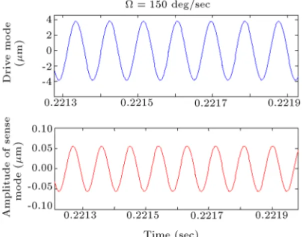
3. Estimating the gyroscope's parameters As mentioned before, knowing the parameters of gy-roscope is benecial for nding the optimum working point of the gyroscope and for improving sensitivity of the gyroscope. If the parameters of gyroscope deviate from the designed value, because of manufacturing tolerances or changes in temperature, humidity, ex-ternal acceleration, etc., the optimum working point will change. If actuation frequency remains at its original value, sensitivity of the gyroscope decreases. By estimating the parameters of the gyroscope, the angular velocity of the gyroscope can be estimated, too. In Table 2, the non-dimensional parameters of a typical parametrically excited gyroscope are presented. In our calculation, the external acceleration on the drive and sense axes is assumed to be 10 g. The angular velocity is 150 deg/sec.
The simulation results of the gyroscope model (Eq. (6)) with the above-mentioned parameters are shown in Figures 5 and 6 for drive and sense directions if the actuation frequency (!) is equal to !y(in normal
and zoomed views).
If !y changes to 1.03 because of environmental
conditions or tolerance errors, the response of the system is like the one shown in Figures 7 and 8. Here, the actuating frequency is equal to the previous !y or
1.0265.
Table 2. Non-dimensional parameters used for parametrically excited gyroscope design.
xy= 0:0001 y= 0:001 x= 0:001
!2
xy= 0:002 !2y= 1:0265 !x2= 1
= 3:8581 10 5
y= 0:001264 x= 0:002303
3= 6:33 10 5 1= 0:0226 0= 0
~ax= 0:0213 ~ay= 0:0213
The amplitude of the sense mode in the system with 3.5% changes in !y decreases signicantly. This
is clear by comparing Figures 7 and 8 with Figures 5 and 6. When ! 6= !y, the amplitude of the sense mode
is 20% of that when ! = !y. Because of this, knowing
some parameters of system like !y is important.
Figure 5. Normal view of drive and sense mode responses when ! = !y.
Figure 6. Zoomed view of drive and sense mode responses when ! = !y.
Figure 7. Normal view of drive and sense mode responses when ! 6= !y.
Figure 8. Zoomed view of drive and sense mode responses when ! 6= !y.
For estimating these parameters, input and out-put of the system should be measured. ~ax and ~ay
(non-dimensional external accelerations in x and y directions) are the system's inputs, and X and Y (displacements of the system in x and y directions) are the system's outputs. The accelerations (inputs) can be fed to the system using the existing accelerometers in the system. The accelerometers exist in most systems where the MEMS gyros are used, for example, in an inertial navigation system. The outputs (X and Y ) are measured with a lock-in amplier [22] that usually exists in an MEMS gyro for determining the amplitude and phase of oscillations.
Parameter estimation will be done using the least squares method. For unbiased estimation of param-eters using least squares method, the inputs should be persistently exciting. The inputs of the system are the non-dimensional external acceleration in the drive and sense modes. The value of non-dimensional acceleration in the \X" and \Y " directions for 10g acceleration is 0.0213 as shown in Table 2. But, this input is constant and probably does not have enough richness to estimate the parameters of the gyroscope. If we notice the system's equations in Eq. (6), there exist some oscillating terms like \21X cos 2!" and
\23X3cos 2!". After beginning the estimation
pro-cess, 1 and 3 will be estimated (not necessarily in a
correct way). \X", \X3", \Y ", and \Y3" are harmonic
because they are the displacement of the proof mass in the drive and sense directions. The proof mass moves in these directions in a sinusoidal way, because the electrostatic excitation term is harmonic. Thus, the multiplication of \X" and \X3" to \cos 2!" will be
harmonic with dierent frequencies that help the inputs to be rich enough to estimate the parameters in an unbiased way.
Now, parameter estimation will be done. As mentioned before, the least squares method is used for estimating the gyroscope's parameters. This method
was rst formulated by Fredrick Gauss in the late 18th century. He used these equations for estimating the orbit of asteroids and planets. In this method, the least squares error of the estimated and real models should be minimized.
From Eq. (7), the estimated parameters can be determined as written in Eqs. (8) and (9). Here, \1"
and \2" are the parameters of the drive and sense
modes' equations, respectively.
1= x (!x2 2+ 21) (xy 2)
(!2
xy 0) (23+x) 21 23 1T;
(8) 2= y (!y2 2) (xy+ 2)
(!2
xy+ 0) y 1T: (9)
Here, state variables of the system are X, X0, Y , and
Y0. The last components of \
1" and \2" are the
coecients of the system inputs that are known, but we estimate them in the identication process.
As can be seen in Eqs. (8) and (9), some pa-rameters can be estimated based on other papa-rameters, e.g. !2
x cannot be estimated individually; it can be
estimated in a summation form (!2
x 2+21). But, it
will be shown that after calculating all the parameters in Eqs. (8) and (9), each parameter can be estimated separately.
The estimator has the following equations in the \least squares error" method.
8 > < > :
_ = Pe = P(Z T)
_P = P PTP
(10) P is the estimation error covariance and is the regression matrix and its components are regression variables in Eq. (10); is a matrix that includes non-dimensional variables that should be identied; Z is the measured output of the system; e is the estimation error; is the forgetting factor that 0 < 1. Here, the measured output consists of outputs in X and Y directions. Measuring the output of the system, one can estimate the unknown non-dimensional parameters using the rst equation in Eq. (10) [23].
Here, two sets of equations like Eq. (10) are written, one for 1and one for 2. Thus Z in Eq. (10)
is X for estimating 1 and Y for estimating 2.
X and Y should be compared with their estimated values for computing the estimation error. The esti-mated values of \X" and \Y " can be obtained using Eq. (11):
^ X = T
1(t)^1;
^ Y = T
where ^1and ^2are estimations of 1and 2(estimated
non-dimensional parameters); T
1(t) and T2(t) will be
in the form shown in Eq. (12). This will be obtained integrating Eq. (6) twice:
T 1(t) =
Rt 0 Xd t R 0 t R 0 Xd t R
0 Y d t
R
0 t
R
0 Y d t R 0 t R 0 X 3d Rt
0 t
R
0 X cos(2!)d t R 0 t R 0 X
3cos(2!)d Rt 0
t
R
0 ~axd
; T
2(t) =
Rt 0 Xd t R 0 t R 0 Xd t R
0 Y d t
R
0 t
R
0 Y d t R 0 t R 0 Y 3d Rt
0 t
R
0 ~ayd
: (12)
\t" is the identication time in Eq. (12). Thus, the error in x and y directions is obtained as follows:
e1= X X;^ e2= Y Y :^ (13)
Using T
1(t) and T2(t) in Eq. (12) results in oscillating
estimated parameters. This is because of the integral form of T
1(t) and T2(t). To prevent this, a stable
polynomial is considered here. This polynomial is (D) = D2 + 3D + 2, where D is the dierential
operator. The rst and second equations in Eq. (6) are considered as P (D)X Z(D)Y f(X; ~ax; ) = 0 and
P0(D)X Z0(D)Y f0(Y; ~ax; ) = 0 in Relation (14),
respectively. The rst and second equations in Rela-tion (14) can be rewritten in the forms of Eqs. (15) and (16). 8 > > > > > > > > > > > > > > > > > > > > > > > > > > > > > > > > > > < > > > > > > > > > > > > > > > > > > > > > > > > > > > > > > > > > > :
P (D)X + Z(D)Y + f (X; ~ax; ) = 0
8 > > > > > > > > > < > > > > > > > > > :
P (D) = D2+ xD +
!2 x 2 z !2 0 + 21
; Z(D) = xy 2!z0
D !2 xy !_z2
0 f (X; ~ax; )=~ax 21X cos 2!
23X3cos 2! (23+x)X3
P0(D)X + Z0(D)Y + f0(Y; ~a
x; ) = 0
8 > > > > > > > < > > > > > > > :
P0(D) = D2+ yD +
!2 y 2 z !2 0 ; Z0(D) = xy+ 2z
!0
D !2 xy+!_2z
0
f0(Y; ~a
x; ) = yY3+ ~ay
(14)
X =(D) P (D)
(D) X
Z(D) (D)Y
f (X; ~ax; )
(D) =T
1(t)1=D2+3D+2D X D2+3D+21 X
D
D2+3D+2Y D2+3D+21 Y D2+3D+21 X3
1
D2+3D+2X cos 2! D2+3D+21 X3cos 2!
1 D2+3D+2~ax
h
3 x 2
!2 x 2 z !2 0 + 21
xy 2!z0
!2 xy !_z2
0
(23+ x)
21 23 1T; (15)
Y =(D) P(D)0(D)Y Z(D)0(D)X f0(Y; ~a(D)y; )
=T
2(t)2=D2+3D+2D X D2+3D+21 X
D
D2+3D+2Y D2+3D+21 Y D2+3D+21 Y3
1
D2+3D+2~ay h3 y 2
!2 y 2 z !2 0
xy+2!0z
!2 xy+!_z2
0 y 1 iT : (16) The above-mentioned method is equivalent to applying a low-pass lter to 1(t) and 2(t) that ignores the
integral terms in these matrices.
Using Eqs. (15) and (16), the new T
1(t) and
T
2(t) will be in the form of Eq. (17). Therefore, the
lter is used for ignoring the integrals in the equations. After using this lter, there will be no pure intergral in the regression matrices, so there is not any wind-up problem and integration error anymore:
T 1(t)=
2
4D2+ 3D + 2D X(t)
| {z }
x5
1
D2+ 3D + 2X
| {z }
x7 D
D2+ 3D + 2Y
| {z }
x9
1 D2+ 3D + 2Y
| {z }
x11 1
D2+3D + 2X3
| {z }
x13
1
D2+3D+2X cos(2!)
| {z }
x15 1
D2+3D+2X3cos(2!)
| {z }
x17
1 D2+3D+2~ax
| {z }
x19 3 5;
T 2(t) =
2
4D2+ 3D + 2D X
| {z }
x21
1
D2+ 3D + 2X
| {z }
x23 D
D2+ 3D + 2Y
| {z }
x25
1 D2+ 3D + 2Y
| {z }
x27 1
D2+ 3D + 2Y3
| {z }
x29
1
D2+ 3D + 2~ay
| {z }
x31
3 5 :
(17) Using new T
1(t) and T2(t), the number of state
variables increases. Each component of these matrices is dened as a new state variable other than previous states (X, X0, Y , Y0). The denition of the new state
variable is shown in Eq. (17) below each component. One of the dened state variables is x5. If one
denes _x5= x6, we have the following equation:
x5= D2+ 3D + 2D X(t); x6= _x5: (18)
Thus:
_x5= x6; _x6= 3x6 2x5+ x2: (19)
The derivatives of x7to x29can be calculated using the
method in Eqs. (18) and (19).
Each component of the matrix P (P1 for the
equation of x direction and P2 for the equation of y
direction) is a state variable, too. As it is shown in Eq. (10), this matrix will be updated with the equation of _P = P P TP .
The stability of the least squares method is proved in the following way:
A positive Lyapunov function is assumed to be in the form of Eq. (20):
V = TP 1; = ^ ! _ = _^: (20)
For (t) to be stable, _V (t) should be negative. Now, _V (t) will be calculated:
_V = 2TP 1_ + T _P 1 ! _V
= 2TP 1P e + T _P 1: (21)
The denition of matrix P is as follows: P =
0 @
Z
0
()T()d
1 A
1
!d P 1
dt =(t)T(t);(22) and:
e = Z T^ = T: (23)
Using the equations in Eq. (10) for updating and P
(with = 0), _V can be found in Eq. (24): _V = 2TP 1P e + TT
= 2Te + TT = eTe 0: (24)
Thus, _V 0 and is stable and bound and so the parameter estimation process is stable, too. Now, if the inputs are persistently exciting, will converge to zero and the parameters will converge to the real parameters. The whole explanations about the sta-bility of least squares method and convergence of the estimated parameters to the real parameters if the input is persistent can be found in [23].
For testing the method of estimation, the compo-nents of 1 and 2 arrays will be changed to 50%.
Using this, we can nd whether the estimator can estimate change of parameters or not.
The identication process is in the way that, rst, the system's equations are written in the form of Eq. (7). Other state variables will be dened by Eq. (17). Updating formulae for matrices P and will be like Eq. (10). After that, the equations will be solved using the initial conditions and the output estimation will be obtained using Eq. (11). The estimation error will be determined by Eq. (13). Estimation of parameters should be done in the way that this error approaches zero with time.
The stability of estimator is studied in [23]. The parameters may not be estimated correctly if the inputs are not persistently exciting.
4. Simulation results
The results of simulations will be shown in this section. Dominating equations for estimator and gyroscope are used for simulation (Eqs. (7), (10), (11), (13), and (17)). The initial conditions of components for matrix P (in Eq. (10)) are assumed to be 104 I
88 for
estimating the parameters in x direction, and 104I 66
for estimating the parameters in y direction, where I88
and I66 are the unity matrices.
Using the non-dimensional parameters in Table 2, the components 1 and 2 can be found as they are
shown in Eq. (25). These components of 1 and 2
arrays change rst +50% and second 50%. Thus, we have three sets of values for 1 and 2 that should
be estimated fast and correctly by the estimator after switching. These dierent sets are given here:
1= 0:001 1:0452 0:002 0:000023
0:00243 0:0452 1:266e 10 4 1;
2= 0:001 1:0265 0:002 0:0000177
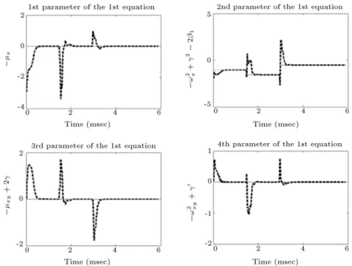
Figure 9. Estimation of the rst to the 4th components of 1. With +50% change:
1= 0:0015 1:5678 0:003 0:0000345
0:0036 0:068 1:899e 10 4 1;
2= 0:0015 1:5398 0:003 0:0000266
0:0023 1: (26)
With {50% change:
1= 0:0005 0:5226 0:001 0:0000115
0:0012 0:023 6:33e 10 5 1;
2= 0:0005 0:5132 0:001 0:00000885
7:685e 10 4 1: (27)
The initial values for 1 and 2 are as follows:
1=0 0 0 0 0 0 0 0:1;
2=0 0 0 0 0 0:1: (28)
The value of in Eq. (10) is set to 0.2.
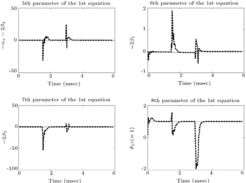
The simulation results are presented in the fol-lowing gures for dierent components of 1 and 2.
Figure 9 for the rst to the 4th and Figure 10 for the 5th to the 8th components of 1, and Figure 11 for the
rst to the 6th components of 2. In these gures, solid
lines are the real values and the dashed lines represent estimated values. The gures show that the estimation algorithm works well when the parameters change.
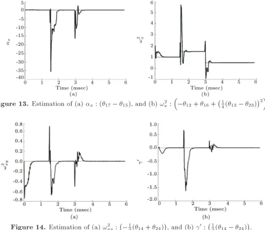
In the next step, for computing each non-dimensional parameter of Table 2, some calculations should be done. For example, using the estimated values for the 4th component of 1 in Eq. (8) and
the 4th component of 2 in Eq. (9), one can
calcu-late xy and . Some parameters like x, y, 1,
y, and 3 are estimated directly because they exist
individually in Eqs. (8) and (9). This is signicant in Figures 9, 10, and 11. Other parameters are !2
x,
, !2
xy, 0, x, !2y, and xy. They are determined
as is written in Table 3. The other non-dimensional parameters in Table 2 will be determined using the above-mentioned method. Figures 12 to 14 show the estimation of non-dimensional parameters of Table 2 (1i is the ith component of 1 and 2i is the ith
component of 2). Solid lines represent real values
and dashed lines represent estimated values. The non-dimensional parameters of Table 2 can be found
Table 3. Finding !2
x, , !2xy, 0, x, !y2, and xyfrom the estimated parameters in Eqs. (8) and (9).
x= 15 23= 15+ 16 = 14(13 23) xy= 12(13+ 23)
!2
xy= 12(14+ 24) !2y= 22+ 2= 22+ 14(13 23)2
0= 1
2(14 24) !2x= 12 21+ 2= 12+ 16+ 14(13 23)
Figure 10. Estimation of the 4th to the 8th components of 1.
Figure 11. Estimation of the 1st to the 6th components of 2.
Figure 13. Estimation of (a) x: (17 15), and (b) !x2:
12+ 16+ 14(13 23)2
.
Figure 14. Estimation of (a) !2
xy: 12(14+ 24)
, and (b) 0: 1
2(14 24)
.
uniquely from the estimated parameters in Eqs. (8) and (9).
As shown in the gures, estimated parameters (dashed line) converge to the true parameters (solid line) in a short time.
5. Implementation remarks
As it is written in the paper, it is necessary to measure X, Y , ~ax, ~ay, and time (t) online and accurate, here.
The oscillation frequency of the proof mass in the gyroscope is more than 10 KHz. If data acquisition is done with the frequency of 500 Hz, there will be 20 oscillations in a sampling period and the results will be in steady state in these oscillations. In this case, using a lock-in amplier can lead to nding the amplitude and phase of the oscillations. The lock-in amplier is an analog circuit with no delay [22]. The accelerations are fed to the system with accelerometer that exists in most systems that use MEMS gyros, for example navigation systems.
6. Conclusion
In this paper, non-dimensional parameters of a para-metrically excited gyroscope were estimated using the least squares method. This estimation is fast and ac-curate. The equations of this gyroscope are nonlinear, but the parameters can be estimated correctly using
this method. In addition, some parameters are rst es-timated in a summation term, but the non-dimensional parameters in these equations are congured in a way that they can be separated and estimated individu-ally. Thus, each non-dimensional parameter can be estimated using the above-mentioned method. The non-dimensional angular velocity is estimated during estimation process that can be used for calculating external angular velocity; the non-dimensional natural frequency of the sense mode is estimated, too. The drive frequency of the system should be equal to this value for having maximum amplitude in the sense mode.
References
1. Nasiri, S., A Critical Review of MEMS Gyroscopes Technology and Commercialization Status, InvenSense, Coronado Drive, Santa Clara, California (2003). 2. Mayagoitia, R.E., Nene, A.V. and Veltink, P.H.
\Ac-celerometer and rate gyroscope measurement of kine-matics: an inexpensive alternative to optical motion analysis systems", Journal of Biomechanics, 35(4), pp. 537-542 (2002).
3. Yazdi, N., Ayazi, F. and Naja, K. \Micromachined inertial sensors", Proceedings of the IEEE, 86(8), pp. 1640-1659 (1998).
gyro-scopes subjected to vibrational frequencies", Sensors and Actuators A: Physical, 125(2), pp. 519-525 (2006). 5. Oropeza-Ramos, L.A., Burgner, C.B. and Turner, K.L. \Robust micro-rate sensor actuated by parametric res-onance", Sensors and Actuators A: Physical, 152(1), pp. 80-87 (2009).
6. Alper, S.E. and Akin, T. \A symmetric surface micromachined gyroscope with decoupled oscillation modes", Sensors and Actuators A: Physical, 97-98(0), pp. 347-358 (2002).
7. Esmaeili, M., Jalili, N. and Durali, M. \Dynamic modeling and performance evaluation of a vibrating beam microgyroscope under general support motion", Journal of Sound and Vibration, 301(1-2), pp. 146-164 (2007).
8. Esmaeili, M., Durali, M. and Jalili, N. \Dynamic modeling and performance evaluation of a vibrating cantilever beam microgyroscope", Proc. 20th Biennial Conference on Mechanical Vibration and Noise, pp. 137-144 (2005).
9. Bhadbhade, V., Jalili, N. and Mahmoodi, S.N. \A novel piezoelectrically actuated exural/torsional vi-brating beam gyroscope", Journal of Sound and Vi-bration, 311(3-5), pp. 1305-1324 (2008).
10. Davis, W.O. and Pisano, A.P. \On the vibrations of a MEMS gyroscope", Proc. International Conference on Modeling and Simulation of Microsystems, pp. 557-562 (1998).
11. Alper, S.E. and Akin, T. \A single-crystal silicon symmetrical and decoupled MEMS gyroscope on an in-sulating substrate", Microelectromechanical Systems, Journal of, 14(4), pp. 707-717 (2005).
12. Alper, S.E. and Akin, T. \Symmetrical and decoupled nickel microgyroscope on insulating substrate", Sen-sors and Actuators A: Physical, 115(2-3), pp. 336-350 (2004).
13. Alper, S.E., Azgin, K. and Akin, T. \A high-performance silicon-on-insulator MEMS gyroscope op-erating at atmospheric pressure", Sensors and Actua-tors A: Physical, 135(1), pp. 34-42 (2007).
14. Yi, R., Han, B., and Sheng, W. \Design on the driv-ing mode of MEMS vibratory gyroscope", Intelligent Robotics and Applications, C. Xiong, H. Liu, Y. Huang, and Y. Xiong, Eds., Springer Berlin Heidelberg, pp. 232-239 (2008).
15. Chang, B.S., Sung, W-T., Lee, J.G., Lee, K-Y. and Sung, S. \Automatic mode matching control loop design and its application to the mode matched MEMS gyroscope", Proc. Vehicular Electronics and Safety, ICVES. IEEE International Conference on, pp. 1-6 (2007).
16. Sungsu, P. and Horowitz, R. \Adaptive control for the conventional mode of operation of MEMS gyroscopes", Microelectromechanical Systems Journal of, 12(1), pp. 101-108 (2003).
17. Oropeza-Ramos, L.A. and Turner, K.L. \Parametric resonance amplication in a MEMS gyroscope", IEEE Sensors, pp. 660-663 (2005).
18. Oropeza-Ramos, L.A., Burgner, C.B. and Turner, K.L. \Inherently robust micro gyroscope actuated by para-metric resonance", Proc. Micro Electro Mechanical Systems, 2008. MEMS 2008. IEEE 21st International Conference on, pp. 872-875 (2008).
19. Pakniyat, A. and Salarieh, H. \A parametric study on design of a microrate-gyroscope with parametric reso-nance", Measurement, 46(8), pp. 2661-2671 (2013). 20. Pakniyat, A., Salarieh, H. and Alasty, A. \Stability
analysis of a new class of MEMS gyroscopes with parametric resonance", Acta Mech., 223(6), pp. 1169-1185 (2012).
21. Zhang, W., Baskaran, R. and Turner, K.L. \Eect of cubic nonlinearity on auto-parametrically amplied resonant MEMS mass sensor", Sensors and Actuators A: Physical, 102(1-2), pp. 139-150 (2002).
22. Maenaka, K., Ioku, S., Sawai, N., Fujita, T. and Takayama, Y. \Design, fabrication and operation of MEMS gimbal gyroscope", Sensors and Actuators A: Physical, 121(1), pp. 6-15 (2005).
23. Astrom, K.J. and Wittenmark, B. Adaptive Control, Prentice Hall (1994).
24. Akin, S.E., and Alper, T. \A single-crystal silicon symmetrical and decoupled MEMS gyroscope on an insulating substrate", Journal of Microelectromechan-ical Systems, 14(14), pp. 707-717 (2005).
25. Akin, S.E. and Alper, T. \A symmetric surface micromachined gyroscope with decoupled oscillation modes", Sensors and Actuators A, 98, pp. 347-358 (2002).
26. Akin, S.E. and Alper, T. \Symmetrical and decoupled nickel microgyroscope on insulating substrate", Sen-sors and Actuators A: Physical, 115(2-3), pp. 336-350 (2004).
Biographies
Zohreh Mohammadi was born in 1985. She received her BS and MS degrees in Mechanical Engineering from Sharif University of Technology in 2006 and 2009, respectively. She is currently a PhD student of Mechanical Engineering and a member of the Center of Excellence in Design, Robotics, and Automation (CEDRA) at Sharif University of Technology, Tehran, Iran. Her research interests include nonlinear dynam-ics, control, MEMS, and adaptive control.
Hassan Salarieh received his BSc degree in Mechan-ical Engineering and, also, Pure Mathematics from Sharif University of Technology, Tehran, Iran, in 2002. He graduated from the same university with MSc and PhD degrees in Mechanical Engineering in 2004 and 2008. At present, he is an Associate Professor in Mechanical Engineering at Sharif University of Tech-nology. His elds of research are dynamical systems, control theory, and stochastic systems.
![Figure 1. Schematics of the designed gyroscope in [6,11,12] and in this paper.](https://thumb-us.123doks.com/thumbv2/123dok_us/8377245.2225263/2.892.479.780.869.1113/figure-schematics-designed-gyroscope-paper.webp)