Sharif University of Technology
Scientia IranicaTransactions B: Mechanical Engineering www.scientiairanica.com
Research Note
Finite volume-lattice Boltzmann modeling of
time-dependent ows
A. Zarghami
a,*and P. Omidvar
ba. Department of Engineering, Science and Research Branch, Islamic Azad University, Fars, Iran. b. Department of Mechanical Engineering, The University of Yasouj, Yasouj, Iran.
Received 18 September 2011; received in revised form 18 December 2012; accepted 12 Murch 2013
KEYWORDS LBM;
Finite volume; Time-dependent ow; Circular cylinder; Mixing layer.
Abstract. In this paper, a stable nite volume formulation of the lattice Boltzmann method is used to study time-dependent ows. For simulation purposes, a cell-centered scheme is implemented to discretize the convection operator and weighting factors are used as ux correctors to enhance the stability. Also, additional lattices at the edge of each boundary cell are used, which allow a much better description of the actual geometrical shape. Compared with previous nite volume formulations, the proposed approach resulted in a wider domain of stability and faster convergence. The scheme is validated through simulations on ow over a circular cylinder and mixing layer ow. The results show that the method is a promising scheme for simulating time-dependent ows.
© 2013 Sharif University of Technology. All rights reserved.
1. Introduction
In recent years, there has been considerable research in developing and expanding the Lattice Boltzmann Method (LBM) for solving dierent uid dynamics problems. The LBM was rst introduced by McNa-mara and Zanetti [1] as an improvement to the method of Lattice Gas Automata (LGA). Later, it was shown that the Lattice Boltzmann Equation (LBE) could be derived from the continuous Boltzmann equation by choosing an appropriate set of discrete velocities, based on some special discretization schemes. This approach helped for better understanding of the basis of LBM, and provided a solid theoretical foundation for LBM [2].
The fundamental idea of the LBM is to construct simplied kinetic models that incorporate the essential physics of microscopic or mesoscopic processes, so that the macroscopic averaged properties obey the desired
*. Corresponding author. Tel.: +98 7284692101-4
E-mail addresses: [email protected] (A. Zarghami); [email protected] (P. Omidvar)
macroscopic equations. The basic premise for using these simplied kinetic-type methods for macroscopic uid ow is that the macroscopic dynamics of a uid are the result of the collective behavior of many mi-croscopic particles in the system and that mami-croscopic dynamics are not sensitive to the underlying details in microscopic physics. By developing a simplied version of the kinetic equation, it is not required to solve complicated kinetic equations such as the full Boltzmann equation, and it is not needed to follow each particle as in molecular dynamics simulations [2].
LBM is based on a microscopic picture but fo-cuses on the averaged macroscopic behavior of the uid. That gives simplicity of implementation, a clear physical picture and fully parallel algorithm. Briey, the advantages of the LBM over the conventional CFD schemes can be summarized as:
I) Simple explicit algorithm;
II) Parallelization capability for doing massively parallel simulations;
IV) Robust simulations for complex uids and etc. [3].
The standard BGK approximation of LBM, based on Single-Relaxation-Time (SRT), was introduced by Qian et al. [4], the latter being based on the original idea of Bhatnagar et al. (1954) [2]. Due to its extreme simplicity, the lattice BGK equation has become the most popular LB model. But, the standard BGK-LBM suers from numerical instabilities that can induce a local blowup of the computation [5]. So, in recent years, intensive studies on stability analysis regarding dierent lattice Boltzmann models have been carried out by various researchers.
The Multiple-Relaxation-Time (MRT) model [6,7], based on the original matrix, a formulation of the LBM, has been proposed as an alternative to the standard BGK model by D'Humieres [6]. In this model, the collision step is performed in moment space, whereas the propagation step is done in discrete velocity space. The MRT models are considerably more stable than the standard SRT model and overcome some obvious defects in the standard BGK model, such as the xed ratio between the kinematic and bulk viscosities [8]. However, the stability properties of the MRT-LB models are still not satisfactory [9]. Thus, the MRT-LBM has been persistently pursued, and much progress has been made [10].
Recently, in order to improve the stability and ac-curacy of the LB schemes, with regards to rough mesh, the Entropic Lattice Boltzmann Method (ELBM) has been developed. The goal of this approach, proposed by Ansumali et al. [11-13], is construction of a scheme that: I) satises the Boltzmann H-theorem and II) shows a higher non-linear stability. In this approach, an entropy function is dened for the kinetic equation and it is ensured, at each iteration step, that the entropy of the system remains non-decreasing (Boltzmann H-theorem). This simple idea renders the method thermodynamically consistent and makes the simulations non-linearly stable. However, ELBM were known only on highly symmetric lattices, such as the 27 velocity lattice (D3Q27). So, in order to increase the
speed of simulations, it is required that the number of discrete velocities be reduced [14].
Another limitation of the standard LBM is the use of uniform Cartesian grids. This limitation is par-ticularly severe in many practical applications where the complex geometry of boundaries cannot be well tted by regular lattices. In order to overcome such limitation and increase computational eciency, locally embedded uniform grids [15,16] and interpolated grid stretching [17,18] have been proposed.
In locally embedded uniform grids, Cartesian meshes are used and grid spacing is divided by an integer (or level of renement) to the next rened
grid level. In this scheme, rened uniform grids and the main coarse grids live on dierent space and time scales. The consequence is that one needs to perform less time steps on the coarse grid than on the ne grid, because also, time is rened locally [19]. In the interpolated grid stretching scheme, interpolations are used at the interface between two connected meshes of dierent grid spacing and at solid boundaries [20]. With the interpolated grid stretching method, one can use the simple bounce-back boundary conditions with body-tted meshes. However, this method re-quires an extra computational eort for interpolation at every time step and it also has a strict restric-tion on the selecrestric-tion of interpolarestric-tion points, which requires upwind 9 points for 2D problems and upwind 27 points for 3D problems if a structured mesh is used [21].
Among recent advances in LB research to handle complex ows, a particularly remarkable option is represented by changing the solution procedure from the original `stream and collide' to a Finite Volume (FV) formulation. The rst attempt to combine the FV method with LBM is attributed to Nannelli and Succi [22]. They obtained a FV-LBM for the volume-averaged coarse-grain distribution function, starting from the discrete velocity Boltzmann equation. Peng et al. proposed a cell-vertex nite volume scheme [23]. This method allows for an arbitrary decomposition of the computational domain into triangular or quadri-lateral elements, with no structural limitations for the mesh. Using the mapped or non-uniform grid for the structured grid is another advantage of this method, which results in a decrease in the number of grid nodes and iterations for desired accuracy.
For the FV-LB methods, one needs to select ecient approaches, such as upwind schemes, to do numerical discretization, in order to get a stable so-lution [24]. Numerical research has shown that these methods have good capabilities in real applications. However, most of the presented FV schemes have several drawbacks with respect to numerical stabil-ity [25].
The primary motivation of this research is to develop a stable FV formulation of the LBM to study global time-dependent ows. The introduction of upwind weighting factors allows overcoming instability and accelerating the convergence process. In this paper, we extended the method to simulate the ow past a circular cylinder and mixing layer ow to study the instability of these ows. The abundant literature on these classical ow problems allows us to carry out extensive benchmarking for this new formulation. Here, we rst describe the LBE, the proposed cell-centered nite-volume scheme and boundary condi-tions. Then, the computational results are presented, followed by the concluding remarks.
2. Lattice Boltzmann-nite volume formulation
2.1. Discrete lattice Boltzmann equation The Boltzmann equation discretized in velocity space, and the collision term modeled with BGK [2] approx-imation, is usually written in the following dierential form:
@fi
@t + ~vi:rfi= 1
(fi fieq) i = 1; :::; n; (1)
where n is the number of dierent velocities in the model, feq is the particle equilibrium distribution
function associated with motion along the ithdirection
in velocity space, ~vi is the velocity in the ithdirection,
is the relaxation time and the right hand side of the equation is the collision operator.
The discrete velocities and the equilibrium distri-bution functions must be chosen appropriately, such that the mass and momentum are conserved and some symmetry requirements are satised. Here, we choose the 2D nine-bit (D2Q9) model with the equilibrium
distribution function dened as: fieq(~x; t) =wi
c1+ c2(~vi:u) + c3(~vi:u)2+ c4(u:u)
; (2)
where c1 = 1; c2 = 1=c2s; c3 = 1=2c4s; c4 = 1=2c2s and
wi is the weighting factor and equals 4/9 for i = 0, 1/9
for i = 1 4 and 1/36 for i = 5 8. The discrete velocities are given by ~vo= 0 and ~vi= i(cos i; sin i)
with i = 1; i = (i 1)=2 for i = 1 4 and
i=p2; i= (i 5)=2 + =4 for i = 5 8 and cs=
c=p3 = 1=p3 is the speed of sound in the model [2]. The macroscopic density, and velocity, u, of the uid are determined by = ifi and u = ifi~vi;
respectively. Also, the corresponding kinematic shear viscosity isrelated to the relaxation time by v = c2
s,
and macroscopic pressure is given by p = c2 s [25].
2.2. FV formulation of LBM
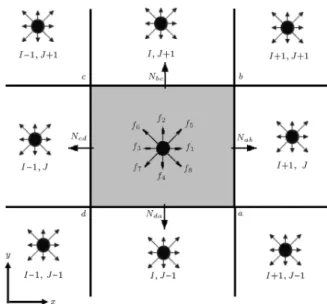
According to Figure 1, the integration of the rst term in Eq. (1), based on the cell-centred nite-volume scheme, is approximated as:
Z
abcd
@fi
@tdA
@fi
@t
I;J
AI;J; (3)
where AI;J is the area of abcd. In the above equation,
fi is assumed to be constant over the area abcd, thus
avoiding a set of equations to be solved. This is a common practice in the nite volume methods [26].
A standard integration of the second term of the left-hand side of Eq. (1) gives the ux associated with the streaming operator of the ith particle distribution
Figure 1. Schematic of the FV discretization with cell-centered lattice.
function through the four edges ab; bc; cd and da. As vix
and viyare constant, the following equation is obtained
after applying Green's theorem: Z
abcd
vi:rfidA =
Z
abcd
@(vix:fi)
@x +
@(fi:viy)
@y
dx dy
= I
around I;J
(vixfidy viyfidx)
[fi]I;J + [f2 i]I+1;Jvi:Nab
+[fi]I 1;J+ [fi]I;J 2 vi:Nbc
+[fi]I;J+ [f2 i]I;J+1vi:Ncd
+[fi]I;J 12+ [fi]I;Jvi:NdaA: (4)
In the above equation, Nk = (yi xj)k is the
outward unit vector normal to the edge, and k = ab; bc; cd; da. This formulation is named the ux averaging scheme, which would diverge if the ux term be weak [27]. This could be avoided by using the divergence theorem and applying an upwind scheme. In this case, the integration of the second term of the left-hand side of Eq. (1) results as follows [24]:
Z
abcd
vi:rfidA =
(
[fi]I;Jvi:Nab if vi:Nab 0
+ (
[fi]I;Jvi:Nbc if vi:Nbc 0
[fi]I;J+1vi:Nbcif vi:Nbc< 0
+ (
[fi]I;Jvi:Ncd if vi:Ncd 0
[fi]I 1;Jvi:Ncdif vi:Ncd< 0
+ (
[fi]I;Jvi:Nda if vi:Nda 0
[fi]I;J 1vi:Ndaif vi:Nda< 0
X
k
~vi:Nk(fi)k: (5)
Now, the following weighting factors are employed in the convective uxes of Eq. (1):
ab= Pppab
horizental; bc=
pbc
P
ptvertical;
cd=Pppcd
horizental; da=
pda
P
pvertical: (6)
where: X
phorizental=
X
(pI+1;J + 2pI;J+ pI 1;J) ;
X
pvertical=
X
(pI;J+1+ 2pI;J+ pI;J 1) ;
and:
pab= pI+1;J pI;J; pbc= pI;J+1 pI;J;
pcd= pI;J pI 1;J; pda= pI;J pI;J 1:
The idea of introducing these factors to improve nu-merical stability without adding articial viscosity is related to the fact that the macroscopic pressure, p, acts as a driving force for the ow between the two cells [28]. So, according to the above relations, the convective uxes may be written as follows:
Si=
Z
~vi:rfidA ~vi:Nab ab[fi]I;J
+ (1 ab)[fi]I+1;J
+ ~vi:Nbc bc[fi]I;J+ (1 bc)[fi]I;J+1
+ ~vi:Ncd cd[fi]I;J+ (1 cd)[fi]I 1;J
+ ~vi:Nda da[fi]I;J
+ (1 da[fi]I;J 1: (7)
The heuristic meaning of these coecients is to enhance transport downhill the pressure gradient and reduce it uphill [29]. Assuming a linear behavior of fi; fieq
within internal cells, the integration of the collision term (right-side term of Eq. (1)) is performed through the following formulation:
Qi= AI;J
1
4[fine]I;J+18
[fne
i ]I+1;J
+ [fne
i ]I;J+1+ [fine]I 1;J+ [fine]I;J 1
+161
[fne
i ]I+1;J 1+ [fine]I+1;J+1
+ [fne
i ]I 1;J+1+ [fine]I 1;J 1
; (8)
where fne
i = fi fieqis the non-equilibrium component
of the distribution function. Note that the integration of the collision terms in boundary cells reduces to the following form:
Qi= AI;J
h
(fi)I;J (fieq)I;J
i
: (9)
As we know truncation or round-o causes error in the numerical solution of partial dierential equations, the solution may go unstable in typical cases (such as ows with strong gradients) unless articial dissipation is explicitly added to the calculation. Note that articial dissipation is the direct result of even order derivatives in modied equation [30]. So, in ux modeling, especially at high Reynolds numbers or in the presence of strong gradients, the addition of articial dissipation is inevitable to perform a stable simulation. Therefore, in order to damp out spurious oscillations the fourth-order articial dissipation takes the following form:
h D(4)f
i
i
I;J =x (r) 2 x [fi]I;J
+ "y (r)2y [fi]I;J; (10)
where "x and "y are damping factors in x and y
directions, respectively, and the integration over each cell is the sum of ux the time updating. These damping factors were adjusted to achieve the desired numerical stability and convergence. In Eq. (10), the fourth-order gradient operator (Nabla-Delta) was discretized in x and y directions as follows:
(r)2x [fi]I;J = [fi]I+2;J 4 [fi]I+1;J + 6 [fi]I;J
4 [fi]I 1;J+ [fi]I 2;J;
(r)2y [fi]I;J = [fi]I;J+2 4 [fi]I;J+1+ 6 [fi]I;J
A modied fth order, Runge-Kutta time dierenc-ing scheme is used to advance the computations in time [28]. Therefore, the new-time particle distribution function is calculated as follows:
fin+1= fn
i + lAt I;J S
l 1 i + Ql 1i
; (12) where n denotes the time step, 1 = 0:0695; 2 =
0:1602; 3= 0:2898; 4= 0:5; 5= 1 and l = 1; :::; 5.
2.3. Boundary conditions
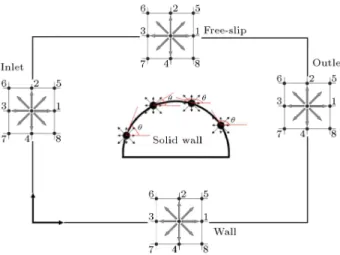
In order to transform hydrodynamic boundary con-ditions to the boundary concon-ditions for the distribu-tion funcdistribu-tions, addidistribu-tional lattices at the edge of each boundary cell are introduced. Then, boundary nodes are treated like internal nodes, except that the uxes over boundary edges also have to be evaluated. The inlet boundary conditions at I = 1 are given by (see Figure 2):
f1= f3+ 2uin=3;
f5= f7+ 0:5(f4 f2) + uin=6;
f8= f6+ 0:5(f2 f4) + uin=6: (13)
The above described scheme is also known as Zou and He boundary conditions, suggesting the name of the original authors proposing this idea. At the outlet boundary, i.e. I = Nx, the distribution functions are
extrapolated as follows:
fi(I =Nx; J) = 1:5fi(I = Nx 1; J)
0:5fi(I = Nx 2; J): (14)
For the free slip boundary condition (Figure 2), the unknown distribution functions are calculated as f8=
f5, f4= f2and f7= f6. This implies no tangential
mo-mentum transfer to the boundary, as required for a free
Figure 2. Physical boundaries of the solution domain and lattice model on typical boundaries.
slip uid motion [31]. Wall boundary conditions are in LB simulations usually implemented by applying the so-called bounce-back rule, which means that incoming particle portions are reected back towards the nodes they came from, and which gives second-order accuracy for straight walls [21]:
f6= f8; f2= f4; f5= f7: (15)
For the arbitrary shaped solid wall, suggests the selection of appropriate fis for extrapolation
pur-poses.
3. Simulation results
First, we applied the model to ow over a circular cylinder and then in the second part, the results for simulating a time-dependent mixing layer ow are presented. In all cases, the results were compared with available well-documented solutions in the liter-ature.
3.1. Flow over circular cylinder
One of the basic time-dependent problems in hydro-dynamics is the ow past a circular cylinder, which has been both numerically and experimentally studied extensively in the past, thus becoming a standard benchmark problem. The ow has been numerically simulated for Reynolds number up to 150. The Reynolds number is calculated as Re = UD=; U being the inlet uniform velocity and D the cylinder diameter.
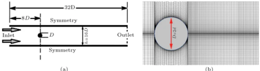
Figure 3(a) shows a schematic of the ow cong-uration and boundary conditions simulated here. The symmetry boundary conditions were used for top and bottom walls. All the simulations have been performed in a large 32D 16D domain so as to minimize the ef-fects of boundaries on the development of the wake. To investigate grid independency, the Wake length (L) was considered at three dierent non-uniform grid points, 150 80; 180 100, and 200 120, at Re=40. It was observed that the grid point of 200120 was suciently ne to ensure a grid-independent solution for laminar ow (see Figure 3(b)). The ow is impulsively started by forcing a uniform prole at the inlet. Then, after reaching the fully periodic solution, we measure and report the length of the wake behind the cylinder, the separation angle and the drag coecient.
The convergence criterion is applied to the veloc-ity eld to ensure that the convergence happens. If the velocity satises this criterion, the program code will go to the next step and the iterations will continue. Generally, the proper equation denes the investigation of the convergence situation for the numerical methods. In other words, the error functions are used for assur-ance that a parameter-like velocity converges. Here, a relative velocity error is applied as follows:
Figure 3. (a) Flow conguration for simulation of ow past a cylinder placed symmetrically in a planar channel. (b) Mesh grids around circular cylinder.
Table 1. Relative velocity error for dierent ux modeling schemes (nite volume formulation).
Flux modeling scheme Relative velocity error
Re = 20 Re = 40 Re = 80 Re = 100
Averaging scheme (Eq. (4)) 1.1E-04 4.5E-04 Diverged Diverged
Upwind scheme (Eq. (5)) 6.4E-04 3.3E-03 8.7E-03 Diverged
Pressured based scheme (Eq. (7)) 4.8E-05 4.6E-05 4.6E-05 4.5E-05 Averaging scheme with articial dissipation ("x= "y= 5) 5.9E-05 6.4E-05 7.3E-05 diverged Pressured based scheme with articial dissipation ("x= "y= 5) 1.4E-05 1.5E-05 1.7E-05 2.5E-05
En+1=
P
I;J
r u2
I;J+vI;J2
n+1 r u2
I;J+vI;J2
n P
I;J
r u2
I;J+ vI;J2
n+1
; (16)
where n and n+1 indicate the reference and under test condition, respectively. Also, u and v are stream-wise and span-wise components of the velocity, respectively. Table 1 compares the relative velocity error of the ow over a circular cylinder for dierent ux modeling schemes. In this table, results are presented in iteration equal to 20000. As seen, applying the pressure based factors enabled us to reach a more stable solution in the mentioned Reynolds numbers. Also, a better conver-gence was achieved by adding the articial dissipation term. This led to an improvement in the stability and accuracy of the numerical scheme and reduction in iteration steps.
Another parameter which has an inuence on the accuracy of the solution is compressibility error, which is related to the fact that the LBE recovers the Navier-Stokes for weakly-compressible ows (Ma<<1). In other words, The LB model is a quasi-compressible uid solver. This means that it enters a slightly compressible regime to solve the pressure equation of the uid. Compressibility eects do, however, impact numerical accuracy. As these eects scale like the square Mach-number, Ma2, they are kept under control
by keeping the Mach number low. The Mach number is nothing else than Uin=cs, which means that it is
proportional to the velocity in the lattice unit, Uin.
So, in all simulations, inlet velocity Uinwas set to 0.03
and, consequently, Mach number was obtained equal to Ma= 0:03 p3 = 0:05.
The results of Figure 4 show the time history of the relative velocity error by adding the arti-cial dissipation to ux averaging and pressure based
Figure 4. Eect of articial dissipation ("x= "y= 5) in numerical convergence of the ow over a circular cylinder: (a) Flux averaging scheme at Re = 80; and (b) pressure based scheme at Re = 100.
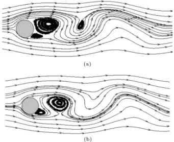
Figure 5. Streamline plot of ow past circular cylinder at Re = 40.
Table 2. Comparison of geometrical and dynamical parameters at Re = 40: L = length of wake, d = cylinder radius, s= separation angle.
Authors L=d s CD
Coutanceau and Bouard [32] 4.26 53.5 -Dennis and Chang [33] 4.69 53.8 1.552 Nieuwstadt and Keller [34] 4.357 53.34 1.550 He and Doolen [35] 4.49 52.84 1.499 Patil and Lakshmisha [36] 4.284 52.74 1.558
Fornberg [37] 4.48 - 1.5
Calhoun [38] 4.36 - 1.62
Ye et al. [39] 4.54 - 1.52
Ubertini et al. [40] - - 1.56
Present work 4.47 52.8 1.551
schemes. Hence, a better convergence was achieved. To conclude, applying the pressure-biasing factors and articial dissipation term enabled us to overcome some shortcomings, especially the numerical instability of nite volume formulations of the lattice Boltzmann method.
Details of the ow path behind the cylinder at the Re=40 are shown in Figure 5. We see that the two vortices in the streamline plot are perfectly aligned, indicating that the ow is stable. Table 2 compares the present numerical results with previous experimental and computational results [32-40]. In particular, the length of the wake behind the cylinder, the separation angle and the drag coecient computed with the present method are in good agreement with the corresponding values available in the literature.
It is generally accepted that the wake of a cylinder immersed in a free-stream rst becomes unstable to perturbations at a critical Reynolds number of about Re = 46 1[39]. Above this Reynolds number, a small asymmetric perturbation in the near wake will grow in time and lead to an unsteady wake and Von Karman vortex shedding. This is indeed what we nd for our simulation at Re = 62, which has been carried out on a 320 240 non-uniform mesh. Figure 6 shows the behavior of the relative velocity error at Re = 60, 62 and 100. For Reynolds higher than 62, we see that the
Figure 6. Behavior of velocities residuals at Re = 60, 62 and 100.
Figure 7. Streamline plot of ow past circular cylinder: (a) Re = 100; and (b) Re = 150.
behavior of relative velocity error is periodic. Figure 7 shows a plot of the streamline pattern for Re = 100 and 150. The vortices in the streamline plot have begun to slide past one another, indicating the onset of vortex shedding, and the zero-contour level has begun to warp. The characteristic vortex shedding is clearly visible in the plots.
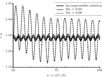
In order to investigate the eect of Mach number on the accuracy of simulation, the time-dependent behavior of drag coecient, CD, at dierent Mach
numbers and Re = 100, are plotted in Figure 8. Results are compared with the incompressible nite dierence solution of Calhoun [38]. From these simulations, it is obvious that the dierence between Ma = 0.03 and the incompressible solution is very low. In this work, values of drag coecient dier from the incompressible solution by a small discrepancy of about 0.86% in the whole periodic region. The dierence between the incompressible result and the case for Ma = 0.08 is equal to 8.8% for average values in the periodic
Figure 8. Time-dependent drag coecient at Re = 100 and dierent Mach numbers. Results compared with incompressible result of Calhoun [38].
Table 3. Comparison of drag coecient for unsteady ow at Re = 100.
Authors CD
Calhoun [38] 1.330 Ding et al. [41] 1.391 Liu et al. [42] 1.350 Braza et al. [43] 1.364 Present work 1.310
region. Therefore, it is shown that the results of the lattice Boltzmann simulation have signicant de-pendence on the chosen Mach number. Thus, the eect of Mach number on the accuracy of the solution should be considered in simulations using LB methods. Table 3 lists quantitative comparisons for the drag coecient.
To determine if we are getting the proper shedding frequency, we compute the non-dimensional shedding frequency, or Strouhal number, given by St = fsD=U,
where fs is the shedding frequency. To compute the
shedding frequency, the periodic evolution of the drag coecient was used. We estimate a non-dimensional Strouhal number of about 0.161 for Re = 100. By comparison, Ding et al. [41] reports a value of St = 0.166, and Liu [42] reports a value of St = 0.164.
Figure 9 represents the St-Re relation for dierent schemes available in the literature. One can clearly nd that, although the results from the dierent schemes deliver very dierent values for the Strouhal number, they all have something in common. The reason is that both Reynolds number and Strouhal number are functions of the inow uniform velocity, U. Generally, the quantitative agreement between our results and other numerical/experimental results is satisfactory, and we conclude that our scheme is correctly capturing the transition from steady to unsteady ow.
Figure 9. Graphical presentation (St-Re) of former studies compared [44-47] with the results from the present works.
Figure 10. Schematic of mixing layer ow. Fast side refers to lower stream and slow side refers to upper stream and refers to the thickness of the mixing layer.
3.2. Time-dependent mixing layer ow
The plane mixing layer is characterized by the merging of two initially unperturbed parallel ow streams with velocities U1 and U2 (see Figure 10). Downstream of
the conuence, the two streams exchange momentum as they come into intimate contact with each other. The mixing layer itself is dened by the region in which this merging process is occurring. In this study, the computational domain is Lx = Ly = 80, where
is the theoretical thickness of the layer in x = Lx
[48]. The theoretical thickness of the mixing layer ow is calculated according to analytical solution, whereas it is estimated based on the inlet velocity prole for mixing layer ows. The system size of the mesh grid is 261 521. In the y direction, an equally spaced grid is used in the mixing layer thickness i.e. for 35 < y < 45, and then the grid is stretched on both sides. Also, in the x direction, the grid is uniform between 0 < x < 5 and then stretched.
The ow is initially at rest (zero speed) and is impulsively started by forcing a hyperbolic prole, such as Uinlet(y) = 0:5 f(1=) + tanh (y)g at the inlet where
= [U2 U1] = [U1+ U2] represents a measure for the
intensity of the layer shearing. The ow has been numerically simulated for a Reynolds number equal to Re = U= = 300, where U = U2 U1.
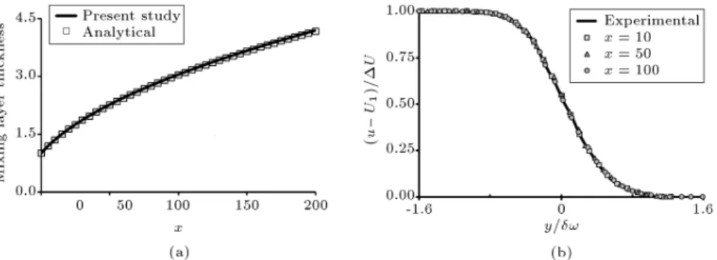
Figure 11. (a) Mixing layer thickness at Re = 300. Curve t using != 0:2875px + 12:371. (b) The variation of the normalized u-component velocity.
When the ow gets steady, the results of the simulation essentially display a laminar growth of the boundary layer. Figure 11(a) illustrates the stream-wise growth of the mixing layer thickness, ! =
1=(@ U=@y)max where the average layer speed, U =
0:5(U1+ U2), is set at 1.5. A square-root relationship
t to these computed results is shown in the graph reported in Figure 11(a). The layer is respondent with classical laminar, square-root growth character-istics [49].
A dimensionless variable that is written as a function of a dimensionless transverse coordinate is called self-similar if the function does not change with the downstream position. Results in self-similar coordinates for the mixing layer were also investigated. The principle of self-similarity as a representation of moving equilibrium was introduced by Townsend [50]. Free shear layers provide an excellent example of this equilibrium, and they form one class of canonical laminar and turbulent ow elds.
In order to verify our results, the present nu-merical results are compared to the experimental data of Oster and Wygnanski [51]. Non-dimensional time-averaged stream-wise velocities obtained by a statistical method at dierent stations are shown in Figure 11(b). This gure clearly shows that the self-similarity of the mixing layer is obtained using LBM, and indicates that the mixing layer is a ow with a self-preserving state.
Now, in order to investigate the unsteady mixing layer ow, the inlet velocity component is superim-posed by some time-dependent perturbations. The perturbations are introduced in the form of a traveling wave. The perturbation, which consists of a com-bination of linear Eigen-functions obtained from the linear stability calculations, is specied for the inow boundary condition. In other words:
v(x; y; t) = A Real[V (y)ei( !t)]; (17)
where V (y) is the velocity Eigen-function correspond-ing to the most amplied mode of the two-dimensional
Figure 12. Velocity time histories at centerline for the u component at stream-wise location, x = 100 and 200.
Orr-Sommerfeld equation, and A is the amplitude of the two-dimensional forcing which corresponds to the fundamental frequency [52]. Figure 12 illustrates the time traces of the stream-wise component of velocity at a selected location in the layer. The gures clearly indicate that the response of the layer is very periodic, which is due to the periodic forcing imposed at the inlet plane of the layer. The peak-to-peak time lapse in these curves provides evidence of the passage of a structure. This time lapse, t, together with an assumed advection speed for these structures of U, allows estimation of the scale of a structure.
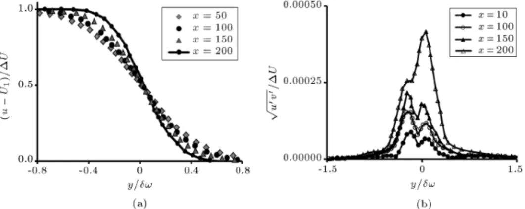
The mean eld statistics for the stream-wise ve-locity component is illustrated in Figure 13(a). Clearly, these results are not representative of a self-similar layer. The lack of self-similarity is apparently as a result of the forcing imposed at the inlet plane. As the ow goes downstream, the distributions become closer together. This is indicating that the ow enters the self-similar region. The Reynolds stress statistics, pu0v0=U, obtained from this simulation
are illustrated in Figure 13(b). Again, these proles do not exhibit self-similar behavior. The distributions are more likely to collapse on each other when far downstream of the ow.
Figure 13. (a) Mean eld statistics for u-component velocity. (b) Reynolds stress distribution.
Figure 14. Eect of articial dissipation term ("x= "y= 7) in numerical convergence of the time-dependent mixing layer ow at Re = 300 using pressure based scheme.
dissipation term in simulating a time-dependent mixing layer ow using a pressure based scheme. Figure 14 compares the convergence of the proposed scheme with and without using the articial dissipation term. Clearly, results highlight the positive eect of the articial dissipation term on the convergence of the solution.
4. Conclusion
A nite volume formulation of LBM is derived, based on a cell centered discretization scheme on structured tessellation. For this purpose, pressure based cor-rection factors, as well as the articial dissipation term, were used to improve stability. Also, consistent boundary conditions have been described. The method was validated by simulating the time-dependent ow over a circular cylinder and a forced mixing layer ow. Comparing the results to the well-documented numerical/experimental data in the literature, good agreement was observed. It was also shown that the scheme is robust and promising in simulating time-dependent ows.
References
1. McNamara, G.R. and Zanetti, G. \Use of the Boltz-mann equation to simulate lattice gas automata". J. Phys. Rev. Let., 61, pp. 2332-2335 (1988).
2. Succi, S. (2001) The Lattice Boltzmann Equation for Fluid Dynamics and Beyond, Oxford University Press, Oxford, UK.
3. Yu, D., Mei, R. and Luo, L.S. \Viscous ow computa-tions with the method of lattice Boltzmann equation", Prog. Aero. Sci., 39, pp. 329-367 (2003).
4. Qian, Y.H., D'Humieres, D. and Lallemand, P. \Lat-tice BGK models for navier-stokes equation", Euro-phys. Lett., 17(6), pp. 479-484 (1992).
5. Succi, S., Karlin, I.V. and Chen, H. \Role of the H-theorem in lattice Boltzmann hydrodynamic simula-tions", Rev. Mod. Phys., 74, pp. 1203-1220 (2002).
6. D'Humieres, D. \Generalized lattice Boltzmann equa-tions", Prog. Aeronaut. Astronaut., 159, pp. 450-458 (1992).
7. Lallemand, P. and Luo, L.S. \Theory of the lattice Boltzmann method: dispersion, dissipation, isotropy, galilean invariance and stability", Phys. Rev. E, 61, pp. 6546-6562 (2000).
8. D'Humieres, D. \Multiple-relaxation-time lattice Boltzmann models in three dimensions", Phil. Trans. R. Soc. Lond. A, 360, pp. 437-451 (2002).
9. Geier, M.C. \Ab initio drivation of the cascade lat-tice Boltzmann", PhD Thesis, University of Freiburg, Freiburg, Germany (2006).
10. Ricot, D., Marie, S., Sagaut, P and Bailly, C. \Lattice Boltzmann method with selective viscosity lter", J. Comput. Phys., 228, pp. 4478-4490 (2009).
11. Ansumali, S. and Karlin, I.V. \Stabilization of the lat-tice Boltzmann method by the Htheorem: A numerical test", Phys. Rev. E, 62(6), pp. 7999-8003 (2002).
12. Ansumali, S. and Karlin, I.V. \Single relaxation time model for entropic lattice Boltzmann methods", Phys. Rev. E, 65, 056312 (2002).
13. Ansumali, S., Karlin, I.V. and Ottinger, H.C. \Mini-mal entropic kinetic models for hydrodynamics", Eu-rophys. Lett., 63(6), pp. 798-804 (2003).
14. Chikatamarla, S., Ansumali, S. and Karlin, I.V. \En-tropic lattice Boltzmann models for hydrodynamics in three dimensions", Phys. Rev. Lett., 97(1), 010201 (2006).
15. Filippova, O. and Hanel, D. \Grid renement for lattice-BGK models", J. Comput. Phys., 147(1), pp. 219-228 (1998).
16. Tolke, J., Freudiger, S. and Krafczyk, M. \An adap-tive scheme using hierarchical grids for lattice Boltz-mann multi-phase ow simulations", Comput. Fluids, 35(8/9), pp. 820{830 (2006).
17. He, X., Luo, L.S. and Dembo, M. \Some progress in lattice Boltzmann method: Part I. Nonuniform mesh grids", J. Comput. Phys., 129, pp. 357-363 (1996).
18. He, X., Luo, L.S. and Dembo, M. \Some progress in lattice Boltzmann method: Enhancement of Reynolds number in simulations", Physica A, 239, pp. 276-285 (1997).
19. Rohde1, M., Kandhai, D., Derksen, J.J. and Van den Akker, H.E.A. \A generic, mass conservative local grid renement technique for lattice-Boltzmann schemes", Int. J. Numer. Meth. Fluids, 51, pp. 439-468 (2006).
20. Bouzidi, M., D'Humieres, D., Lallemand, P. and Luo, L.S. \Lattice Boltzmann equation on a two-dimensional rectangular grid", J. Comput. Phys., 172, pp. 704-717 (2001).
21. Shu, C., Niu, X.D. and Chew, Y.T. \Taylor-series expansion and least-squares-based lattice Boltzmann method: two-dimensional formulation and its applica-tions", Phys. Rev. E., 65, 036708 (2002).
22. Nannelli, F. and Succi, S. \The lattice Boltzmann equation on irregular lattices", J. Stat. Phys., 68, pp. 401-407 (1992).
23. Peng, G., Xi, H., Duncan, C. and Chou, S-H. \Finite volume scheme for the lattice Boltzmann method on unstructured meshes", Phys. Rev. E., 59, pp. 4675-4682 (1999).
24. Stiebler, M., Tolke, J. and Krafczyk, M. \An upwind discretization scheme for the nite volume lattice Boltzmann method", Comput. Fluids, 35, pp. 814-819 (2006).
25. Ubertini, S. and Succi, S. \Recent advances of lattice Boltzmann techniques on unstructured grids", Prog. Comput. Fluid Dyn., 5(1/2), pp. 85-96 (2005).
26. Zarghami, A., Ubertini, S. and Succi, S. \Finite vol-ume lattice Boltzmann modeling of thermal transport in nanouids", Comput. Fluids, 77, pp. 56-65 (2013).
27. Hirsch, C. \Numerical computation of internal and ex-ternal ows", Fundamentals of Numerical Discretiza-tion I, John Wiley, Chichester, UK (1988) .
28. Razavi, S.E., Ghasemi, J. and Farzadi, A. \Flux mod-eling in the nite volume lattice Boltzmann approach", Int. J. Comput. Fluid D., 23(1), pp. 69-77 (2009).
29. Zarghami, A., Maghrebi, M.J., Ubertini, S. and Succi, S. \Modeling of bifurcation phenomena in suddenly expanded ows with a new nite volume lattice Boltz-mann method", Int. J. Mod. Phys. C, 22(9), pp. 977-1003 (2011).
30. Tanehill, J.C., Anderson, D.A. and Pletcher, R.H. Computational Fluid Mechanics and Heat Transfer, pp. 101-126, Taylor & Francis, USA (1997).
31. Zarghami, A., Maghrebi, M.J., Ghasemi, J. and Uber-tini, S. \Lattice Boltzmann nite volume formulation with improved stability", Commun. Comput. Phys., 12(1), pp. 42-64 (2012).
32. Coutanceau, M. and Bouard, R. \Experimental deter-mination of the main features of the viscous ow in the wake of a circular cylinder in uniform translation. Part 1. Steady ow. Part 2. Unsteady ow", J. Fluid Mech, 79, pp. 231-256 (1977).
33. Dennis, S.C.R. and Chang, G.Z. \Numerical solutions for steady ow past a circular cylinder at Reynolds numbers up to 100", J. Fluid Mech., 42, pp. 471-489 (1970).
34. Nieuwstadt, F. and Keller, H.B. \Viscous ow past cir-cular cylinders", Comput. Fluids, 1, pp. 59-71 (1973).
35. He, X. and Doolen, G. \Lattice Boltzmann method on curvilinear coordinates system: Flow around a circular cylinder", J. Comput. Phys., 134, pp. 306-315 (1997).
36. Patil, D.V. and Lakshmisha, K.N. \Finite volume TVD formulation of lattice Boltzmann simulation on unstructured mesh", J. Comput. Phys., 228, pp. 5262-5279 (2009).
37. Fornberg, B. \A numerical study of steady viscous ow past a circular" J. Fluid Mech. 101, pp. 583-587 (1980).
38. Calhoun, D. \A Cartesian grid method for solving the two-dimensional streamfunction-vorticity equations in irregular regions", J. Comput. Phys., 176(2), pp. 231-275 (2002).
39. Ye, T., Mittal, R., Udaykumar, H. and Shyy, W. \An accurate cartesian grid method for viscous incom-pressible ow with complex immersed boundaries", J. Comput. Phys., 156, pp. 209-240 (1999).
40. Ubertini, S., Succi, S. and Bella, G. \Lattice Boltz-mann schemes without coordinates", Phil. Trans. R. Soc. Lond. A, 362, pp. 1763-1771 (2004).
41. Ding, H., Shu, M. and Ca, Q.D. \Application of stencil-adaptive nite dierence method to incompressible viscous ows with curved boundary", Comput. Fluids, 36, pp. 786-793 (2007).
42. Liu, C., Zheng, X. and Sung, S.H. \Preconditioned multi-grid methods for unsteady incompressible ows", J. Comput. Phys., 139, pp. 35-57 (1998).
43. Braza, M., Chassaing, P. and Ha Minh, H. \Numerical study and physical analysis of the pressure and velocity elds in the near wake of a circular cylinder", J. Fluid Mech., 165, pp. 79-130 (1998).
44. Persillon, H. and Braza, M. \Physical analysis of the transition to turbulence in the wake of a circular cylin-der by three-dimensional Navier-Stokes simulation", J. Fluid Mech., 365, pp. 23-88 (1998).
45. Karniadakis, G.M. and Triantafyllou G.S. \Three-dimensional dynamics and transition to turbulence in the wake of blu objects", J. Fluid Mech, 238, pp. 1-30 (1992).
46. Thompson, M., Hourigan, K. and Sheridan J. \Three-dimensional instabilities in the wake of a circular cylinder", Experimental Thermal and Fluid Science, 12, pp. 190-196 (1996).
47. Williamson, C.H.K. \Dening a universal and contin-uous Strouhal-Reynolds number relationship for the laminar vortex shedding of a circular cylinder", Phys. Fluids, 31(10), pp. 2742- 2744 (1998).
48. Schlichting, Boundary Layer Theory, Springer (2005).
49. Lowery, P.S. and Reynolds, W. \Numerical simulation of spatially developing forced plane mixing layer", NASA Technical Report NCC2-015, USA (1986).
50. Townsend, A.A.R. The Structure of Turbulent Shear Flow, Cambridge University Press, Cambridge, UK (1956).
51. Oster, D. and Wygnanski, I. \The forced mixing layer between parallel streams", J. Fluid. Mech., 123, pp. 91-99 (1982).
52. Maghrebi, M.J. and Zarghami, A. \DNS of forced mixing layer", Int. J. Numer. Anal. Mod., 7(1), pp. 173-193 (2010).
Biographies
Ahad Zarghami obtained a PhD degree in 2012 from Shahrood University of Technology, Shahrood, Iran, and is Assistant Professor in the Department of Engi-neering at the Fars Science and Research Branch of the Islamic Azad University. He is currently undertaking a post-doctoral fellowship in H2CU Honors Center of Italian Universities, La Sapienza University of Rome, Italy. His research interests include computational uid dynamics, lattice Boltzmann method, nanouids and heat transfer.
Pourya Omidvar obtained a PhD degree, in 2010, from the University of Manchester, UK, under the supervision of Prof. Peter K. Stansby and Dr. Benedict D. Rogers mostly focused on extreme waves loading on wave-energy devices and wave-body interactions. He has been one of the contributors for the open-source code SPHysics. The code SPHysics, which is a SPH (Smoothed Particle Hydrodynamics) code, has been developed jointly in Manchester in cooperation with reputed institutions in the world. He was also employed by EPFL, Switzerland in 2010 and 2011. and is currently Assistant Professor at the State University of Yasouj, Iran. His research interests include numerical modeling, meshless and particle methods, Smoothed-Particle Hydrodynamics (SPH), Lattice Boltzmann Method (LBM), free-surface ow and uid-structure interaction.