Methodology for bus layout for topological quantum error correcting codes

(1)

R E S E A R C H

Open Access

Methodology for bus layout for

topological quantum error correcting codes

Martin Wosnitzka, Fabio L Pedrocchi

*

_{and David P DiVincenzo}

*_{Correspondence:}

[email protected] JARA Institute for Quantum

Information, RWTH Aachen University, Aachen, 52056, Germany

Abstract

Most quantum computing architectures can be realized as two-dimensional lattices of qubits that interact with each other. We take transmon qubits and transmission line resonators as promising candidates for qubits and couplers; we use them as basic building elements of a quantum code. We then propose a simple framework to determine the optimal experimental layout to realize quantum codes. We show that this engineering optimization problem can be reduced to the solution of standard binary linear programs. While solving such programs is a NP-hard problem, we propose a way to ﬁnd scalable optimal architectures that require solving the linear program for a restricted number of qubits and couplers. We apply our methods to two celebrated quantum codes, namely the surface code and the Fibonacci code.

Keywords: topolocial quantum error correcting codes

1 Introduction

Since the theoretical demonstration of fault-tolerant quantum information processing, a holy grail of modern physics has been to realize fault-tolerant quantum computing archi-tectures in the lab. While this still remains a very challenging task, many experimental advances have been achieved. Arguably, one can hope to see the ﬁrst small-size imple-mentations in a near future.

Among the most promising quantum computing platforms, one ﬁnds so called topo-logical quantum codes []. The main idea is to encode quantum information (in the form of logical qubits) using a large number of physical qubits. The additional degrees of free-dom introduced in the Hilbert space then allow the extraction of some information about the errors induced by the environment (the error syndrome) and to correct them with-out collapsing the stored logical qubit. Furthermore, topological codes are, by deﬁnition, immune to local and static perturbations [].

Most of the topological quantum codes are realizable as a lattice of qubits (some of them might require qudits instead) that are coupled to each other. Depending on the speciﬁcs of the quantum code, one qubit might be coupled to several other qubits in its neighborood. In this work, we present a general framework to determine the optimal architecture to couple the qubits of a quantum code. Here we assume that couplers can be introduced be-tween qubits and we identify the coupling architecture that minimizes the total length of the couplers, rendering the physical implementation more practical. Our analysis is valid for any quantum code and we show that this set of optimization problems are identical to

(2)

well-known binary linear programs. We would like to point out that our choice of metric deﬁning what we call anoptimalscheme might turn out not to be the one that experimen-talists will eventually consider relevant. Experimental and theoretical works with several qubits per transmission lines have just started, [–] and the results obtained from experi-ments will be crucial to determine which optimality criteria should be satisﬁed in practice. In this context, our work builds a methodology where a huge number of layouts can be studied and from which an optimal layout can be determined; this methodolody applies to a variety of metrics and not only to the precise choice we have made here. We thus believe that it represents a useful tool.

We apply our formalism to two celebrated quantum codes, namely the surface code [, ] and the Fibonacci Levin-Wen code [, ]. The former one is a planar version of Kitaev’s toric code [] that is among the most promising quantum computing platforms because of its simplicity and its surprisingly high error threshold of about %. The latter code is more involved but supports Fibonacci anyons that are universal for topological quantum computation; in other terms every quantum gate can be approximated to any accuracy by braiding Fibonacci anyons. Since the Fibonacci model is universal, it can hardly be simu-lated on a classical computer. In order to determine the error threshold of the Fibonacci Levin-Wen model, one would probably need to perform a full quantum simulation and thus have a quantum computer at hand. However, what precise algorithm should be run on the hypothetical quantum computer is still open and is a very interesting problem. Re-cently, some speciﬁc limiting cases where the Fibonacci model can be simulated classically have been investigated where the error threshold is approximatively . % [].

We think that our work on the surface code is particularly timely since the ﬁrst set of experiments to build small fragments of surface code (with  data qubits) have now started []. It is thus interesting to understand what architecture is optimal and could be realized in the lab. Finally we compare our results for the surface code with previously suggested architectures [, ].

The paper is organized as follows. In Section . we present the physical model under consideration for a generic quantum code as well as the formalization of the optimization problem. In particular, we show that the optimal architecture is found by solving binary linear programs. In Section . we apply the formalism developed in Section . in order to find an optimal architecture for the Fibonacci code. In particular, we present a methodol-ogy to find scalable architectures by solving tractable binary linear programs. Section . finally contains our results for the surface code.

2 Connecting qubits optimally

In this work, we consider Transmon Qubits (TQs) and Transmission Line Resonators (TLRs) as the prototypical examples of physical qubits and moderate distance couplers [, ]. However, it is worth pointing out that our approach does not depend on the tech-nological details of the implementation but can be applied to any kinds of qubits and cou-plers [–].

2.1 Model

Consider a set of N TQs q, . . . ,qN that lie on a two-dimensional plane at positions

x, . . . , xN. Depending on the speciﬁc quantum codes that one wants to realize, see

(3)

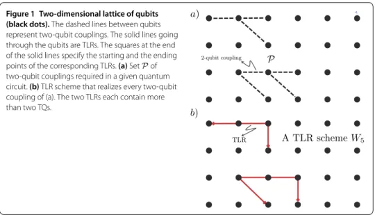
Figure 1 Two-dimensional lattice of qubits (black dots).The dashed lines between qubits represent two-qubit couplings. The solid lines going through the qubits are TLRs. The squares at the end of the solid lines specify the starting and the ending points of the corresponding TLRs.(a)SetPof two-qubit couplings required in a given quantum circuit.(b)TLR scheme that realizes every two-qubit coupling of (a). The two TLRs each contain more than two TQs.

through TLRs. As any quantum circuit can be reduced to a succession of single- and two-qubit operations [], the most straightforward approach is to introduce TLRs containing each exactly two TQs; in this way TLRs realize the setPof all two-qubit couplings neces-sary to implement a given quantum circuit, see Figure .

However, using a new TLR for each pair of qubits that should be coupled to participate in two-qubit gate operations might not be the most optimal approach to this engineering problem. In fact TLRs are able to couple to more than two TQs and we assume thatm individual TQs can reside inside the resonant cavity provided by the TLR. Each of the TQs can be controlled separately and coupled to any of the otherm–  TQs through the TLR. Following recent experimental progress [], we find thatm≤ is a realistic upper bound. Informative micrographs of TLRs hosting several TQs can be found in [] and on page  of [] or in Figure (a) of []. Also, it seems natural to restrict the number pof TLRs that are connected to a single TQ; here we choosep=  []. We would like to mention here thatX-mon qubits, a type of transmon qubit, are specifically designed so that they can couple to several TLRs, see Figure  in [] for example where each branch of theX-mon can be coupled to a different TLR.

We call an unordered sequence of sitesik∈ {, . . . ,N} a stringS={i,i, . . . ,im}. The

length|S|of a string is deﬁned by the number of sites it contains. To each stringS, we as-sociate a numberκ_S= , ; ifκ_S= , then a TLR is present and hosts themTQsqi, . . . ,qim, otherwise no single TLR hosts all those speciﬁcmqubits. We denote bySmthe set of all

stringsSwith|S| ≤m. We call the vector

Wm= (κ{,}, . . . ,κ{N–,N};κ{,,}, . . . ;κ{,,...,m}, . . .)T ()

a TLR scheme. We say that a TLR corresponding to a stringSisincludedin a TLR scheme WmifκSis one of the elements of the vectorWm. We say that a TLR schemeWmcontains

a TLR associated with stringSif it is included andκ_S= .

In order to formalize the concept ofoptimalTLR scheme, we introduce a costC_S ∈R associated with each stringS∈Sm. The cost vector of the schemeWmis then

(4)

Using this notation, the total cost of a given TLR schemeWmisC(Wm)T·Wm. The goal of

this work is to determine one TLR schemeWmthat minimizes the cost and realizes the set

P of two-qubit couplings. In Sections  we present concrete examples of cost functions for the surface code and for the Levin-Wen model.

The problem of ﬁnding the TLR schemeWm that has minimal cost is solved by using

standard binary linear optimization methods. The problem is formalized as follows:Given a set of two-qubit connectionsP, and given two integers m and p, ﬁnd the TLR scheme Wm

that minimizes the costC(Wm)T·Wmsuch that

. For allij∈ {, , . . . ,N},

S∈Sm|ij∈S

κ_S≤p. ()

. Wmrealizes every two-qubit coupling ofP.

It is worth pointing out again that the maximal numbermof qubits per TLR, as well as the maximal numberpof TLR per qubit, is ﬁxed.

It is now clear why we call this abinarylinear program; every component of the vector Wmis either  or . Solving such a binary linear program is generally very diﬃcult and is in

fact an NP-hard problem. However, speciﬁc instances of such problems can be tractable, and we give explicit examples below. As a side remark, note that when all the numbers in the program are allowed to be real, then the situation is dramatically simpliﬁed and the optimization problem can be solved in polynomial time.

In this work, we use the free software lpsolve, available at http://lpsolve.sourceforge.net/ ./, to find the optimal solution to the binary linear program defined above. In order to simplify the program, we leave out all thesuperfluousTLRs. We call a TLR superfluous if it can be replaced by two (or more) TLRs that host no common qubits such that the same set of required two-qubit couplings is realized; one can thus always replace a superfluous TLR by two TLRs that will have a lower overall cost.

As mentioned in the Introduction, we aim to ﬁnd the optimal architectures for two important quantum error correcting codes, namely the surface code and the Levin-Wen model. We ﬁnd interesting that such quantum technological problems can be turned into standard optimization problems.

3 Application to Quantum error correcting codes

3.1 Fibonacci Levin-Wen model

Levin-Wen models are a class of spin systems deﬁned on trivalent lattices whose excita-tions realize any consistent (Abelian or non-Abelian) anyonic theory []. Here we focus on a particular Levin-Wen model, namely the Fibonacci Levin-Wen model [, ]. Its name takes its origin in the nature of the excitations above the ground states; indeed they are Fibonacci anyons with topological chargeτ and fusion rules

τ×τ=  +τ. ()

(5)

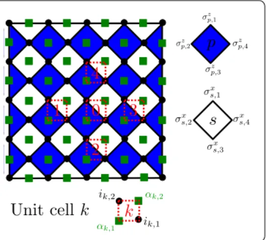
Figure 2 The Fibonacci Levin-Wen model is deﬁned on a trivalent lattice.Each edge hosts a spin-1/2 particle (a so-called data qubit) depicted here by a black dot.(a)Vertexvwhere three edges of the lattice meet. The state of the three qubits at the vertexvis|ijk.(b)Twelve data qubits (black dots) needed to deﬁne the plaquette operatorBp

on the trivalent lattice. In order to perform non-demolition measurements of vertex and plaquette operators, one introduces ancillary qubits (green squares). Hereα0is used to measureBp,

while the remaining ancillary qubitsα1–6are used to measure the six vertex operators. This number of additional qubits is appropriate for the plaquette reduction method of Ref. [9].

Considering a trivalent lattice with each edge carrying a spin-/ particle, we deﬁne the Fibonacci Levin-Wen Hamiltonian [, ],

H= –

v

Qv–

p

Bp, ()

whereQvandBpare operators that are respectively associated with vertexvand plaquette

pof the lattice, see Figure .

The vertex operatorQvacts on the three qubits residing on the edges that meet at

ver-texv. If the states of the three qubits on theses edges are|i,|j, and|k, then we have

Qv|ijk=δijk|ijk, ()

with

δijk=

⎧ ⎨ ⎩

 ifijk= , , , , ,

 otherwise. ()

The plaquette operators are more complicated and involve -qubit interactions. Consider the twelve qubitsa–andi–around a given plaquettep, see Figure (b). The plaquette operators are then deﬁned through

Bp=

  +φ

B_p+φBτ p

, ()

withφ=+ √



 the golden ratio and

Bs_p|a, . . . ,a,i, . . . ,i=

i_,...,i_

Bs,i

,...,i

p,i,...,i(a, . . . ,a)a, . . . ,a,i

, . . . ,i, ()

wheres= ,τand

Bs,i

,...,i

p,i,...,i(a, . . . ,a) =F aii sii F

aii sii · · ·F

aii si_i F

aii

(6)

For the Fibonacci theory we have []

Fττ τ τ=

φ– _φ–/

φ–/ –φ–

, ()

and all otherF’s are trivial. One can then show that the Levin-Wen plaquette and star operators satisfy [Bp,Qv] = [Bp,Bp] = [Qv,Qv] = , for allv,v,p,p[, ].

We deﬁne the Fibonacci code []F(an example of a stabilizer code) as the ground-state subspace of Hamiltonian (), namely

F=|ψ|Qv|ψ=Bp|ψ=|ψ,∀p,v. ()

On a surface with nontrivial topology this ground-state subspace of Hamiltonian () is degenerate and one uses this set of states to encode logical qubits. A nontrivial op-eration (a logical error) applied to the logical qubit is implemented by creating pairs of

τ-excitations, braiding them, and annihilating them. The logical operation does not de-pend on the details of the braiding process, but only on its topology; this is in fact the main idea of topological quantum computation []. Importantly, Fibonacci anyons are universal for quantum computation and any quantum gate can thus be performed in a topologically protected fashion.

Recently, Ref. [] has shown how to explicitly construct quantum circuits that measure plaquette and vertex operators of the Fibonacci Levin-Wen model; this is required to mea-sure the error syndrome ofFand to decide how to perform error correction. Here we go one step further and determine the optimal qubit-coupler architecture to realize those quantum circuits. It is not the goal of the present work to review in detail how vertex and plaquette quantum circuits are constructed. But these circuits indicate which qubits must be coupled and this indicates the binary linear program of Section  that is to be solved to obtain the optimal architecture. For the sake of completeness in Figure  we reproduce the circuit of Ref. [] for theplaquette reductionmethod.

We note here that ancillary qubits are needed to perform non-demolition measurements ofQvandBp. According to the plaquette reduction method of Ref. [], in Figure  the

ancillary qubitαis used to measureBp, while the ancillary qubitsα–are used to measure the six vertex operatorsQv.

Here we choose the cost functionC_S that measures the geometric length of the TLR corresponding toS={i,i, . . . ,im},

CS=min_σ

_m

k=

|xiσ(k)– xiσ(k–)|

, ()

whereσ is a permutation ofmelements.

Said diﬀerently,C_Sis the geometric length of the shortest path going through all the TQs speciﬁed in the stringS. In this work we thus look for the TLR scheme that minimizes the total length of the TLR wires.

(7)

Figure 3 Figure reproduced with permission from Ref. [9]: quantum circuit for the plaquette reduction method. (a)Full circuit for the plaquette reduction method to calculate the value of the plaquette operatorBp. The numbering of the qubits is that of Figure 2(b). The individual gates of the circuit are detailed

in (b).(b)Each element of the circuit in (a) is reduced toX-gates,S-gates, single qubit rotationsR(ρyˆ) by an angleρalong they-axis, controlled-Xgates, controlled-Sgates, and Toﬀoli gates.

Having in handPreduction, we can solve the binary linear program of Section  and de-termine the optimal TLR scheme. The result is summarized in Table  and a pictorial representation is given in Figure .

For completeness, we also investigate the plaquette swappingmethod of Ref. [] to measure plaquette operators. In this case, more ancillary qubits are required, see Figure . For the sake of completeness, in Figure  we reproduce the plaquette swapping circuit of Ref. []. The setPswapping of two-qubit couplings required by the plaquette swapping method is summarized in Table . Again, we solve the binary linear program and ﬁnd the optimal architecture of Table ; here we have again chosenm=p= . As the pictorial representation would be too crowded, we refrain from drawing the TLRs corresponding to Table .

.. Scaling

(8)

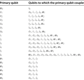
Table 1 We list the setPreductionof all the two-qubit couplings required to measure the plaquettepand the six vertex operators of Figure 2, following the plaquette reduction method of Ref. [9]

Primary qubit Qubits to which the primary qubit couples

α0 i6

a1 a6,i1,i2,i6,α1

a2 i1,i2,i3,i6,α2

a3 i2,i3,i4,i6,α3

a4 i3,i4,i5,i6,α4

a5 i4,i5,i6,α5

a6 a1,i1,i2,i6,α6

i1 a1,a2,a6,i2,i3,i6,α1,α6

i2 a1,a2,a6,i1,i3,i4,i6,α1,α2

i3 a2,a3,a4,i1,i2,i4,i5,i6,α2,α3

i4 a3,a4,a5,i2,i3,i5,i6,α3,α4

i5 a4,a5,i3,i4,i6,α4,α5

i6 α0,a1,a2,a3,a4,a5,a6,i1,i2,i3,i4,i5,α5,α6

α1 a1,i1,i2

α2 a2,i2,i3

α3 a3,i3,i4

α4 a4,i4,i5

α5 a5,i5,i6

α6 a6,i1,i6

The data and ancillary qubits are labeled according to the notation of Figure 2.

Table 2 Information about the optimal TLR scheme obtained by solving the binary linear program for the measurement of the plaquette operatorBpand the six vertex operatorsQvof Figure 2, following the plaquette reduction method of Ref. [9]

Length of the TLR wire Qubits contained inside the TLR wire

2.52 a.u. a6,α0,i6,α6,i1 4.73 i6,a6,a1,i2,a2 3.15 i1,i2,a2,α2,i3 4.73 i2,i3,α3,i4,a3 3.15 i3,a3,a4,i5,i6 3.15 i6,α5,a5,i5,i4

1.15 i1,α1,a1

1.15 i4,α4,a4

0.58 i2,α1

0.58 i5,α4

In particular, all the two-qubit couplings ofPreductionin Table 1 are realized: there are no more than ﬁve TQs in each TLR, and each TQ couples to maximally four TLRs. A pictorial representation of this TLR scheme and of the arbitrary unit (a.u.) is given in Figure 4.

the lattice. In such a scenario, it is possible to identify a small number of qubits that we couple optimally and that we translate to cover the whole lattice. The aim of this section is thus to introduce a simple method to optimally solve a given unit cell of the model that can be scaled up by simple translation to build a large two-dimensional lattice, see Figure . For the sake of simplicity, we just focus here on the plaquette swapping method of Ref. []. In Table  we present the setP

(9)

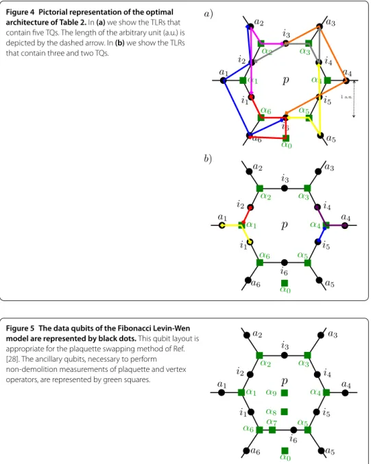
Figure 4 Pictorial representation of the optimal architecture of Table 2.In(a)we show the TLRs that contain ﬁve TQs. The length of the arbitrary unit (a.u.) is depicted by the dashed arrow. In(b)we show the TLRs that contain three and two TQs.

Figure 5 The data qubits of the Fibonacci Levin-Wen model are represented by black dots.This qubit layout is appropriate for the plaquette swapping method of Ref. [28]. The ancillary qubits, necessary to perform non-demolition measurements of plaquette and vertex operators, are represented by green squares.

qubitsi,andi,, see Figure . It is straightforward to see that after translating unit cell  onto unit cell , a TLR will be doubled. In order to avoid such doublings, one needs to slightly modify the algorithm as follows.

Consider a given unit cell  and two distinct stringsS andS that each containsat least onesite inside unit cell . We say thatS={i,i, . . . ,im}andS={j,j, . . . ,jm}are equivalent if∀k∈[,m]∃∈[,m] such that

(10)

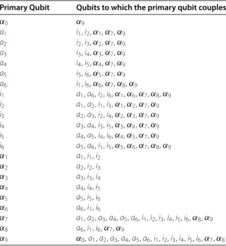
Table 3 The setPswappingof all the two-qubit couplings required to measure the plaquettep and the six vertex operators of Figure 5, following the plaquette swapping method of Ref. [28]

Primary Qubit Qubits to which the primary qubit couples

α0 α9

a1 i1,i2,α1,α7,α9

a2 i2,i3,α2,α7,α9

a3 i3,i4,α3,α7,α9

a4 i4,i5,α4,α7,α9

a5 i5,i6,α5,α7,α9

a6 i1,i6,α6,α7,α8,α9

i1 a1,a6,i2,i6,α1,α6,α7,α8,α9

i2 a1,a2,i1,i3,α1,α2,α7,α9

i3 a2,a3,i2,i4,α2,α3,α7,α9

i4 a3,a4,i3,i5,α3,α4,α7,α9

i5 a4,a5,i4,i6,α4,α5,α7,α9

i6 a5,a6,i1,i5,α5,α6,α7,α8,α9

α1 a1,i1,i2

α2 a2,i2,i3

α3 a3,i3,i4

α4 a4,i4,i5

α5 a5,i5,i6

α6 a6,i1,i6

α7 a1,a2,a3,a4,a5,a6,i1,i2,i3,i4,i5,i6,α8,α9

α8 a6,i1,i6,α7,α9

α9 α0,a1,a2,a3,a4,a5,a6,i1,i2,i3,i4,i5,i6,α7,α8

The data and ancillary qubits are labeled according to the notation of Figure 5.

Table 4 The optimal TLR scheme obtained by solving the binary linear program for the measurement of the plaquette operatorB_pand the six vertex operatorsQ_vof Figure 5, following the plaquette swapping method of Ref. [28]

Length of the TLR wire Qubits contained inside the TLR wire

2.52 a.u. α9,α8,i6,α0,a6

2.84 a1,i1,α7,α8,α9

4.04 α7,α9,i4,i3,a3

4.30 α9,α7,a5,i5,a4

2.44 i1,α7,α6,i6,a6

2.15 i2,α1,i1,a1

2.15 i3,α2,i2,a2

3.04 α7,α9,i2,a2

2.15 i5,α4,i4,a4

1.63 i5,α5,i6,a5

1.15 i4,α3,a3

0.58 i3,α3

In particular, all the two-qubit couplings ofPswappingin Table 3 are realized: there are no more than ﬁve TQs in each TLR, and each TQ couples to maximally four TLRs.

be doubled. Having set these deﬁnitions, we present the steps that we follow to ﬁnd the optimal scalable TLR without doubled TLRs.

• Consider the setP_swapping of two-qubit couplings that contains at least one qubit in the unit cell .

• DeﬁneWas the set of TLR schemes that include all TLRs that are not superﬂuous with respect toP_swapping and all their equivalent TLRs.

• Out of every set of equivalent TLRs, choose one unique representative TLR. For each TLR schemeWm∈W, deﬁne an associated TLR schemeBm. This schemeBmincludes

(11)

Figure 6 Figure reproduced with permission from Ref. [28].Quantum circuit for the plaquette swapping method of Ref. [28]. The qubits labeling is the one of Figure 5. The individual elements of the circuits can be found in Figure 3.

Figure 7 Trivalent lattice on which the Levin-Wen model is deﬁned.The lattice is obtained by translating the unit cell 0 by the unit vectorsv1andv2. For example, the unit cell 1 is obtained by translating unit cell 0 by –v2. For the sake of clarity, we do not represent all the qubits of the lattice. Instead, we draw and label the data (black dots) and ancillary (green squares) qubits of a given unit cellk. This qubit layout is appropriate for the plaquette swapping method [28].

equivalent TLR and are contained inWmas well as all representatives for whichWm

contains at least one equivalent TLR. We call this new set of TLR schemesB. • For each TLR schemeBm∈B, deﬁne a new TLR schemeVmthat includes the same

TLRs asBmand contains all the TLRs that are contained inBmas well as all

equivalent TLRs.

• Perform the linear optimization overBto ﬁnd a TLR schemeBmthat minimizes the

costC(Bm)t·Bmsuch that

. Vmrealizes every two-qubit coupling ofPswapping . . For allij∈ {, , . . . ,N},

S∈Sm|ij∈S

(12)

Table 5 The setP_swapping0 of two-qubit connections between qubits in unit cell 0 of Figure 7 and the remaining qubits of the lattice, following the plaquette swapping method of Ref. [28]

Qubitqin unit cell0 Qubits to whichqcouples

i0,1 α0,7,i0,6,α0,8,α0,9,i1,5,α1,4,i1,6,α1,9,α2,7,i2,5,α2,5,i2,6,α2,9,i6,6,α6,9

i0,5 α0,7,α0,5,α0,4,i0,6,α0,9,α4,7,i4,1,i4,6,α4,7,α4,9,i5,1,i5,6,α5,9,i6,6,α6,9

i0,6 α0,7,i0,1,i0,5,α0,8,α0,9,i1,5,α2,7,i2,5,α3,7,i3,1,i3,5,α4,7,i4,1,i5,1

α0,0 α0,9

α0,4 i0,5,α4,7,i4,1

α0,5 α0,7,i0,5,i5,1

α0,7 i0,1,i0,5,α0,5,i0,6,α0,8,α0,9,i1,5,α1,4,i1,6,α1,9,i5,1,i5,6,α5,9,i6,6,α6,9

α0,8 α0,7,i0,1,i0,6,α0,9,i1,5,

α0,9 α0,7,i0,1,i0,5,α0,0,i0,6,α0,8,i1,5,α2,7,i2,5,α3,7,i3,1,i3,5,α4,7,i4,1,i5,1 4 α0,7,i0,1,α0,8,α1,4

3 i0,5,α0,5,α0,4

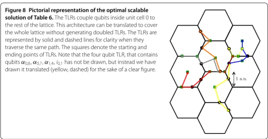
Table 6 Optimal TLR scheme for the set of couplingsP_swpapping0 , i.e., for couplings between qubits in the unit cell 0 and the rest of the lattice

Length of the TLR Qubits contained inside the TLR wire

3.57 a.u. i0,6,α0,9,i2,5,α3,7,i3,1 3.15 α1,9,α1,7,i1,6,i1,5,α0,7 3.48 α2,7,α2,5,i0,1,α0,9,i0,6 2.52 i0,5,α4,0,i4,6,α4,8,α4,9 3.80 i17,1,i6,6,α6,9,i5,1,i0,5 1.44 α0,8,α0,7,α1,4,i0,1

1.15 α0,4,i0,5,α0,5

By translating this TLR scheme to the remaining unit cells of the lattice, one obtains an optimal TLR scheme for the entire lattice that avoids doubled TLRs.

Figure 8 Pictorial representation of the optimal scalable solution of Table 6.The TLRs couple qubits inside unit cell 0 to the rest of the lattice. This architecture can be translated to cover the whole lattice without generating doubled TLRs. The TLRs are represented by solid and dashed lines for clarity when they traverse the same path. The squares denote the starting and ending points of TLRs. Note that the four qubit TLR, that contains qubitsα0,8,α0,7,α1,4,i0,1has not be drawn, but instead we have drawn it translated (yellow, dashed) for the sake of a clear ﬁgure.

Following the above algorithm, we ﬁnd the scalable optimal architectures presented in Table  and Figure .

3.2 Surface code

(13)

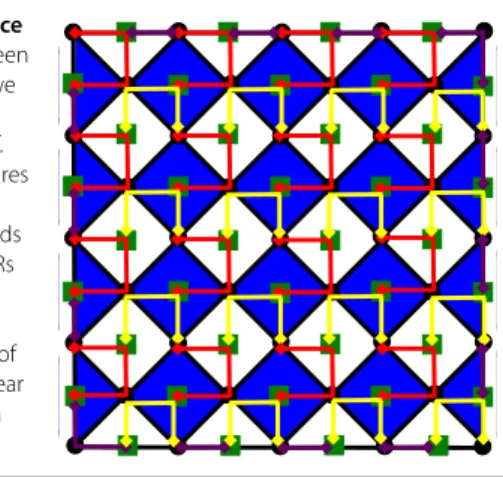
be-Figure 9 Pictorial representation of the surface code.Data qubits reside on the vertices of the lattice and are here depicted by black dots. Products of data qubits around dark (light) squares

correspond to plaquette (star) operators. The green squares are ancillary qubits necessary to measure plaquette and star operators in a non-demolition fashion. We choose the unit cell 0 (dashed square) to generate the whole lattice by translations. The two data qubits and the two ancillary qubits of a unit cell are labeled as shown in the ﬁgure. This choice of boundary conditions leads to a twofold degeneracy of the surface codeSin Eq. (18).

Table 7 The setP_surface0 of couplings between qubits of the unit cell 0 and the rest of the lattice to measure plaquette and star operators of the surface code, see Figure 9

Qubitqin unit cell0 Qubits to whichqcouples

i0,1 α0,1,α0,2,α3,1,α2,2

α0,1 i0,1,i0,2,i1,1,i2,2

i0,2 α0,1,α0,2,α1,2,α4,1

α0,2 i0,1,i0,2,i4,1,i3,2

cause experimental groups are nowadays starting to build small fragments of the surface code.

Consider a square lattice with a spin-/ particle on each vertex, see Figure . We deﬁne the star operatorsAsand plaquette operatorsBpof the surface code as

As=σsx,σsx,σsx,σsx,, ()

Bp=σpx,σpx,σpx,σpx,, ()

wheresandplabel respectively light and dark squares of the lattice, see Figure . Note that plaquette and star operators at the boundaries are products of three qubit operators and not four as is the case in the bulk. Similar to the Fibonacci code, we deﬁne the surface codeSas

S=|ψ|As|ψ=Bp|ψ=|ψ,∀p,s. ()

With the boundary conditions represented in Figure , the surface code is twofold degen-erate and can thus encode a logical qubit []. Similar to the Fibonacci code, the surface code is a topological code and it is thus protected against local (static) perturbations. Its most striking property is its surprisingly high error threshold of about %, see Ref. [] for a detailed review on this subject.

Here we do not review the construction of quantum circuits to measure star and pla-quette operators of the surface code, rather, using the notation of Figure , in Table  we show the setP

surfaceof two-qubit couplings required to measure the eigenvalues ofAsand Bpin a scalable manner []. As was the case for the Fibonacci code, we need to introduce

(14)

Figure 10 Optimal scalable TLR scheme for the surface code.The problem is ﬁrst solved for the couplings between qubits of unit cell 0 and the rest of the lattice, and then we have translated the result to cover the whole lattice. This results is equivalent to the one originally proposed in Ref. [13]. The TLRs are represented by solid lines and the squares denote the starting and ending points of TLRs. Note that rotating each individual four-qubit TLR by 90 degrees leads obviously to another optimal solution. The two-qubit TLRs on the edges and the three-qubit TLRs on the corners (purple) have been put by hand, since a full optimization solution of a smaller surface code lead to such a pattern of boundary two- and three-qubit TLRs. Indeed, it seems clear that this solution at the boundaries remains optimal for a larger surface code.

Solving the binary linear optimization problem withm= , we ﬁnd the scalable optimal TLR scheme reported in Figure . The result is that each bulk TLR hosts four TQs and each bulk TQ is hosted by two TLRs. Interestingly, this result is the one originally proposed in Ref. [], see also Ref. []. We point out that the optimal architecture of Figure  is clearly valid for the smallest possible surface code (consisting of  data qubits and  ancillary qubits) able to detect and correct a single physical qubit error. In fact, we have solved our optimization problem for this small surface code directly and obtained the solution of Figure  with two- and three-qubit TLRs at the boundaries.

.. Distancesurface code

As a ﬁnal relevant explicit example, we consider a surface code that can correct two physi-cal errors. While the surface code depicted in Figure  would contain  data qubits and  ancillary qubits in order to detect and cure two physical errors, there are simple methods to reduce the number of qubits while keeping the distance the same []. Such modiﬁ-cations are important for small-scale implementations of surface codes in a near future; indeed there is clearly an intention to realize a quantum code that requires the smallest possible amount of resource. Here we follow the approach of Ref. [] and consider the ro-tated surface code of Figure . The qubits that are part of the roro-tated code reside inside the black square and some of the boundary ancillary qubits are also incorporated to measure the boundary stabilizers. As was shown in Ref. [], such rotated surface code can correct two physical qubit errors although it possesses many fewer than  data qubits, in fact it consists only of  data qubits and  ancillary qubits. Furthermore, one can do slightly better by requiring not each stabilizer to have its individual ancillary qubit but instead by re-using an ancillary qubit to measure several stabilizer operators. We thus remove the  ancillary qubits with a (yellow) cross in Figure .

We can now solve the linear binary program and ﬁnd the optimal architecture given in Figure .

4 Conclusions

(15)

Figure 11 Pictorial representation of the rotated surface code.The black dots represent data qubits and the green squares ancillary qubits. The rotated surface code [30] contains all the qubits inside the solid square as well as the ancillary qubits surrounded by a black line. In this case, the rotated surface code contains 25 data qubits and 24 ancillary qubits; each ancillary qubit is used to measure exactly one stabilizer. However, one can slightly improve the resource needed by re-using ancillary qubits; we associate many of the ancillary qubits to more than one plaquette and star operator

measurements. We thus remove the ancillary qubits with a yellow cross. Here we list which qubits replace the crossed qubits in the syndrome-computation circuit: qubit 2 is replaced by qubit 3, qubit 5 is replaced by qubit 6, qubit 7 is replaced by qubit 8, qubit 10 is replaced by qubit 11, qubit 13 is replaced by qubit 14,

qubit 15 is replaced by qubit 16, qubit 17 is replaced by qubit 1, qubit 18 is replaced by qubit 3, qubit 19 is replaced by qubit 4, qubit 20 is replaced by qubit 12, qubit 21 is replaced by qubit 16, qubit 22 is replaced by qubit 14, qubit 23 is replaced by qubit 14, qubit 24 is replaced by qubit 6.

Figure 12 Optimal TLR scheme for the rotated surface code of Figure 11, able to detect and correct two physical qubit errors.The TLRs are represented by solid lines with starting and ending points depicted by squares.

We show that ﬁnding such optimal scheme reduces to solve standard binary programs. What optimal means here depends obviously on the choice of a cost function. While we decided to choose to optimize over the total length of transmission line resonators for the Fibonacci and surface codes, our formalism is general enough to be straightforwardly applicable to many other codes and cost functions. While further experimental and theo-retical studies will be necessary to determine which cost function will turn out to be most relevant in practice, we believe that our work represents a useful methodology to inves-tigate a large number of layouts and ﬁnd an optimal one according to some metric. In particular, we show how to apply our method to a restricted set of qubit and couplers that can be scaled up to a large two-dimensional structure.

Competing interests

The authors declare that they have no competing interests.

Authors’ contributions

(16)

Acknowledgements

We are happy to thank N Breuckmann and B Criger for useful discussions. We are grateful for support from the Alexander von Humboldt foundation, ScaleQIT, and QALGO.

Received: 2 November 2015 Accepted: 24 February 2016 References

1. Terhal BM. Quantum error correction for quantum memories. Rev Mod Phys. 2015;87:307.

2. Chow JM. Quantum information processing with superconducting qubits. PhD dissertation, Yale University. 2010. http://www.eng.yale.edu/rslab/papers/jmcthesis.pdf.

3. Ristè D, Poletto S, Huang M-Z, Bruno A, Vesterinen V, Saira O-P, DiCarlo L. Detecting bit-ﬂip errors in a logical qubit using stabilizer measurements. Nat Commun. 2015;6:6983.

4. Yang C-P, Su Q-P, Zheng S-B, Nori F. Entangling superconducting qubits in a multi-cavity system. New J Phys. 2016;18:013025.

5. Ristè D. Feedback control of superconducting quantum circuits. PhD dissertation, TU Delft University of Technology. 2014. http://repository.tudelft.nl/view/ir/uuid%3A787bc488-96b2-4e03-abbe-0a9fba2c4d75/.

6. Bravyi SB, Kitaev AY. Quantum codes on a lattice with boundary. arXiv:quant-ph/9811052 (1998).

7. Freedman MH, Meyer DA. Projective plane and planar quantum codes. Found Comput Math. 2001;1:325-32. 8. Koenig R, Kuperberg G, Reichardt BW. Quantum computation with Turaev-Viro codes. Ann Phys. 2010;325:2707-49. 9. Bonesteel NE, DiVincenzo DP. Quantum circuits for measuring Levin-Wen operators. Phys Rev B. 2012;86:165113. 10. Kitaev AY. Fault-tolerant quantum computation by anyons. Ann Phys. 2003;303:2-30.

11. Burton S, Brell CG, Flammia ST. Classical simulation of quantum error correction in a Fibonacci anyon code. arXiv:1506.03815 (2015).

12. Kelly J, et al.. State preservation by repetitive error detection in a superconducting quantum circuit. Nature. 2015;519:66-9.

13. DiVincenzo DP. Fault-tolerant architectures for superconducting qubits. Phys Scr T. 2009;137:014020.

14. Ghosh J, Fowler AG, Geller MR. Surface code with decoherence: an analysis of three superconducting architectures. Phys Rev A. 2012;86:062318.

15. Blais A, Gambetta J, Wallraﬀ A, Schuster DI, Girvin SM, Devoret MH, Schoelkopf RJ. Phys Rev A. 2007;75:032329. 16. DiCarlo L, Chow JM, Gambetta JM, Bishop LS, Johnson BR, Schuster DI, Majer J, Blais A, Frunzio L, Girvin SM,

Schoelkopf RJ. Demonstration of two-qubit algorithms with a superconducting quantum processor. Nature. 2009;460:240-4.

17. Childress L, Sørensen AS, Lukin MD. Mesoscopic cavity quantum electrodynamics with quantum dots. Phys Rev A. 2004;69:042302.

18. Burkard G, Imamoglu A. Ultra-long-distance interaction between spin qubits. Phys Rev B. 2006;74:041307(R). 19. Trif M, Golovach VN, Loss D. Spin dynamics in InAs nanowire quantum dots coupled to a transmission line. Phys Rev

B. 2008;77:045434.

20. Trifunovic L, Dial O, Trif M, Wootton JR, Abebe R, Yacoby A, Loss D. Long-distance spin-spin coupling via ﬂoating gates. Phys Rev X. 2012;2:011006.

21. Shulman MD, Dial OE, Harvey SP, Bluhm H, Umansky V, Yacoby A. Demonstration of entanglement of electrostatically coupled singlet-tripel qubits. Science. 2012;336:202-5.

22. Trifunovic L, Pedrocchi FL, Loss D. Long-distance entanglement of spin qubits via ferromagnet. Phys Rev X. 2013;3:042023.

23. Hassler F, Catelani G, Bluhm H. Exchange-interaction of two spin qubits mediated by a superconductor. arXiv:1509.0638 (2015).

24. Nielsen MA, Chuang IL. Quantum computation and quantum information. Cambridge: Cambridge University Press; 2000.

25. Levin MA, Wen X-G. String-net condensation: a physical mechanism for topological phase. Phys Rev B. 2005;71:045110.

26. Bonderson PH. Non-Abelian anyons and interferometry. PhD dissertation, California Institute of Technology. 2007. http://resolver.caltech.edu/CaltechETD:etd-06042007-101617.

27. Nayak C, Simon SH, Stern A, Freedman M, Das Sarma S. Non-Abelian anyons and topological quantum computation. Rev Mod Phys. 2008;80:1083-159.

28. Feng W, Bonesteel NE, DiVincenzo DP. Non-Abelian errors in the Fibonacci Levin-Wen model. In preparation. 29. Dennis E, Kitaev A, Landahl A, Preskill J. Topological quantum memory. J Math Phys. 2002;43:4452-505. 30. Horsman C, Fowler AG, Devitt S, Van Meter R. Surface code quantum computing by lattice surgery. New J Phys.