4741.pdf

(1)

Conditional Betas: Asymmetric Responses to Good and Bad

News

Fernando Daniel Chague

A dissertation submitted to the faculty of the University of North Carolina at Chapel Hill in partial fulfillment of the requirements for the degree of Doctor of Philosophy in the Department of Economics.

Chapel Hill 2012

Approved by:

Eric Ghysels

Eric Renault

Saraswata Chaudhuri

Jonathan Hill

(2)

Abstract

FERNANDO DANIEL CHAGUE: Conditional Betas: Asymmetric Responses to Good and Bad News.

(Under the direction of Eric Ghysels.)

In this dissertation we propose a theoretical model for conditional betas. Within a rational

expectation equilibrium model, we provide a precise characterization of the dynamics of betas

and the price of beta risk in terms of the model’s primitive parameters and state variables.

The expressions reveal that during periods of higher uncertainty, the investor requires a higher

market premium. Likewise, the conditional betas also respond to levels of uncertainty;

de-pending on the cash-ﬂow properties of the asset, the asset’s beta can increase or decrease on

higher uncertainty. Because of the connection with uncertainty, conditional betas derive the

stochastic properties from investor beliefs. One of such properties is the asymmetric response

to positive and negative news.

We also provide empirical evidence of the model’s predictions about the dynamics of betas.

For this empirical investigation, we propose an econometric speciﬁcation that provides

time-varying estimates of betas and relates them, non-linearly, to investor beliefs. As a by-product,

we suggest proxies for investor beliefs and uncertainty that can be extracted from stock returns.

The dynamics implied by the estimated parameters conﬁrms the model’s prediction that value

(3)

Acknowledgments

First and foremost, I thank my advisor Eric Ghysels for all the valuable guidance and help

during the development of this dissertation. It was a privilege and a great opportunity working

with him.

I also deeply thank Eric Renault, from whom I learned a lot on the many great courses

he taught us. I wish to express my sincere gratitude to Saraswata Chaudhuri for sharing

his experiences with me, helping me during the very busy times, and giving me very useful

feedbacks.

I thank Jonathan Hill, Michael Aguilar and Christian Lundblad, for contributing with

helpful comments and ideas concerning my work. I also would like to express my gratitude

to Helen Tauchen and all the faculty of the University of North Carolina at Chapel Hill for

allowing me to pursue my academic ambitions.

Special thanks to my colleagues, Racha Moussa, Guansong Wang, Kenneth Reddix and

Justin Contat for the academic and non-academic discussions, and particularly to David

Fragoso Gonzalez, who also helped me a lot in the important stages of this work.

Finally, I would like to express my heartfelt thanks to my beloved wife and family for the

(4)

List of Tables

2.1 NBER Business Cycles and Book-to-Market Portfolios Log-Dividend Growth . . . . 30

2.2 Calibration Parameters, Model and Sample Moments . . . 31

2.3 Time Series Simulations . . . 32

2.4 Asymmetric Volatility . . . 33

2.5 Asymmetric Covariance. . . 34

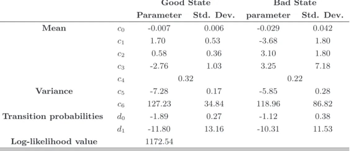
3.1 Markov-Switching Model . . . 60

3.2 Descriptive Statistics of Beliefs and Uncertainty Proxies . . . 61

3.3 5 Book-to-Market Portfolios Conditional Betas . . . 62

3.4 Book-to-Market, Size, Momentum and Industry Portfolios Betas (Beliefs) . . . 63

3.5 Book-to-Market, Size, Momentum and Industry Portfolios Betas (Uncertainty) . . . 64

3.6 Conditional Price of Risk – Beliefs . . . 65

3.7 Conditional Price of Risk – Uncertainty . . . 66

3.8 Asymmetric Betas –β₊+(c) andβ₋−(c) . . . 67

3.9 Asymmetric Betas –β+(c) and β−(c) . . . 68

3.10 Asymmetric Betas –β+₍_c₎ _and_β−₍_c₎ _{. . . 69}

4.1 Beta Decomposition – Descriptive Statistics . . . 89

4.2 Cross Section Sorting – NYSE, Amex and Nasdaq (1963-2009) . . . 90

4.3 Fama-Macbeth Regressions – NYSE (1963-2009) . . . 91

4.4 Determinants ofβ₊− – NYSE (1963-2009) . . . 92

(7)

List of Figures

2.1 Theoretical Expressions Conditional onπt . . . 35

2.2 Impulse Response Functions . . . 36

3.1 Markov-Switching Implied Beliefsπˆt . . . 70

3.2 Estimates of Model (M1) of Conditional Betas (1956-2010). . . 71

3.3 Estimates of Model (M1) of Conditional Betas (1956-2010 excl. years 1997-2001) . . 71

3.4 Joint Conﬁdence Region for Model (M2) withU Ct=V XIt . . . 72

3.5 Conditional Market Betas of Book-to-Market Sorted Portfolios . . . 73

3.6 Conditional Market Betas of Size Sorted Portfolios . . . 74

3.7 Conditional Market Betas of Momentum Sorted Portfolios . . . 75

3.8 Conditional Market Betas of Industry Portfolios . . . 76

3.9 Upside and Downside Betas of Size, Book-to-Market and Momentum Portfolios . . . 77

3.10 Upside and Downside Betas of Industry Portfolios. . . 78

4.1 Four-Fold decomposition – Equally-Weighted . . . 94

(8)

Chapter 1 Introduction

It has long been acknowledged that the systematic risk of stocks, as measured by the market

beta, is time-varying. In empirical applications as early as Fama and MacBeth (1973), betas

were already computed from rolling-sample moments. However, the conditional Capital Asset

Pricing Model (CAPM), that usually motivates time-varying betas, does not provide any hint

on how betas ought to be estimated. In fact, not much is known about what makes betas

vary over time and across assets. An evidence of this is that rolling betas are still used in

empirical applications. Indeed, based on such rolling betas, Lewellen and Nagel (2006) have

condemned the conditional CAPM, by claiming it cannot explain the returns on momentum

and book-to-market portfolios. In order to give the conditional CAPM a fair trial, and also to

improve the measurement of systematic risk, a better understanding of the dynamics of market

betas is urged. The goal of this dissertation is to provide a step in this direction.

In Chapter 2, we derive new theoretical expressions for market betas based on a rational

expectation equilibrium model. The central assumption of the model is the uncertainty faced

by the investor about the true proﬁtability of the assets, which can take on two forms,

depend-ing on the state of the economy. Usdepend-ing the available information, the investor learns about the

state of the economy, and optimally allocates wealth across the assets. In the rational

expecta-tion equilibrium that results, expected returns derive their stochastic properties from investor

beliefs, and can be decomposed into exposures to market risk and hedging risk. The market

risk of an asset is derived from its comovement with the market portfolio, and the hedging risk,

(9)

The two peculiarities of this factor decomposition are the following. First, it says what the

hedging risk is. The Intertemporal Capital Asset Pricing model (ICAPM) of Merton (1973)

does not specify it and, as a result, empirical applications of the ICAPM, and of multifactor

models in general, typically justify risk factors from empirical considerations1. Second, it

provides a functional form for conditional betas and prices of risk. Since the model solves asset

prices in closed-form formulas2, the covariance of returns and prices of risk are also obtainable

in closed-form formulas. As a result, conditional betas and prices of risk are linked to the

model’s primitive parameters and to the stochastic properties of investor beliefs. This, again,

contrasts with the lack of characterization of the dynamics of beta risk in the ICAPM and also

in the conditional CAPM.

In Chapter 2 we also verify the model’s pricing predictions by means of a simulation. We

calibrate an economy with ﬁve assets, each set to resemble one of the ﬁve book-to-market

sorted portfolios. For a reasonable choice of the primitive parameters, which include the

risk-aversion parameter, the assets cash-ﬂow parameters, and the probabilities driving the states

of the economy, the model can reproduce the unconditional excess returns and, to a certain

degree, the variance of excess returns of the actual data. Given the diﬃculties in reconciling,

within an equilibrium framework, the equity premium puzzle — that forces a large risk aversion

parameter — and the excess volatility puzzle — that results in incompatible volatility of returns

and dividends — the fact that the model matches the (unconditional) equity premia of a

cross-section of assets with reasonable parameters is remarkable.

The following empirical implications arise from this calibration. First, a conditional CAPM,

with the deﬁned beta dynamics, provides an appropriate representation of expected returns.

Some empirical studies on the conditional CAPM have assumed away the hedging factors, such

as Jagannathan and Wang (1996), but here this approximation is based within a formal model.

Second, conditional market betas are time-varying and non-linearly related to investor beliefs.

1_{For example, the variables from the predictability literature, such as the price-dividend ratio and the term}

spread, are usually taken as the proxies driving the investment opportunity set. Also, the cross-section anomalies summarized by Fama and French (1993) motivate the size- and value-related factors of risk that now constitute the Fama-French three factor model.

(10)

This non-linearity can be approximated by a monotonic relation of betas with uncertainty,

where by uncertainty we mean the distance of investor beliefs probabilities from the high

certainty cases. Third, the conditional betas of value and growth portfolios have opposing

dynamics; value betas arehigher during high uncertainty periods while growth betas arelower

during high uncertainty periods.

Our model also suggests a diﬀerent interpretation3 for the relevance of return asymmetries

to risk and to asset pricing. The particular sign of returns matters because it can signal a

potential change in the economic conditions. In particular, the average negative news, weighted

by a signal-to-noise ratio, increases uncertainty, whereas the average positive news decreases

uncertainty. Since betas and prices of risk depend on the level of uncertainty, asymmetries

also arise in expected returns. One of the extra features of this interpretation is that it also

identiﬁes which assets are more susceptible to pricing asymmetries — those with cash-ﬂows

that are very sensitive to shifts in the economic conditions.

The last two chapters of this dissertation are devoted to the investigation of the model’s

main empirical implications using data from U.S. stock markets.

In Chapter 3 we explore two aspects of the dynamics of betas: i) how betas relate to diﬀerent

levels of investor beliefs, and ii) how betas relate tochanges in investor beliefs, where changes in

beliefs are proxied by shocks in return. The results reveal diﬀerent asymmetric patterns across

portfolios, particularly across those associated with the pricing anomalies. For instance, among

book-to-market portfolios, value betas are higher during high uncertainty periods, while growth

betas are lower during high uncertainty periods. This empirical ﬁnding, albeit marginally

signiﬁcant, corroborates the calibration results in Chapter 2. Among momentum portfolios,

a clear pattern emerges that distinguishes the risk dynamics of past-winners and past-losers

portfolios. Past-winners betas tend to be lower during periods of high uncertainty, while

past-losers betas tend to be higher during periods of high uncertainty.

3_{The usual justification for the relevance of return asymmetries to asset pricing resides on investor asymmetric}

(11)

The asymmetric patterns with respect to changes in beliefs are also diﬀerent across

portfo-lios. Among size portfolios, small ﬁrms are particularly riskier during negative news markets

than during positive news markets. Among book-to-market portfolios, value ﬁrms also display

higher betas during negative news markets, and this asymmetry further increases with the

relevance of negative news. Interestingly, the asymmetric patterns on the industry portfolios

are less clear, which indicates that the size, book-to-market and momentum anomalies may be,

at least partially, related to misspeciﬁed beta asymmetries.

In Chapter 4 we dissect betas according to the signs of market and asset returns, and

further unveil the asymmetries in betas. The suggested decomposition of betas into signed

betas holds, as a special case, the upside and downside betas of Ang, Chen, and Xing (2006).

For this exploratory task, we consider all common stocks on the Center for Research in Security

Prices (CRSP) dataset, that were listed on the NYSE, Nasdaq and Amex markets. The results

point to a potential asymmetry related to the beta computed on positive market and negative

asset returns that cannot be explained by the measures of risk commonly considered by the

(12)

Chapter 2 Theoretical Model

2.1 Introduction

The conditional Capital Asset Pricing Model (CAPM) does not impose any structure on how

be-tas should vary. This has largely been tackled from an empirical perspective. Early parametrical

approaches include the multivariate GARCH framework (Bollerslev, Engle, and Wooldridge,

1988) and the instrumental variables betas (Harvey (1989), Harvey and Kirby (1996)). Recent

parametric models suggest treating conditional betas as latent variables: Adrian and Franzoni

(2009) suggest using the Kalman ﬁlter while Ang and Chen (2007) apply Markov-chain

Monte-Carlo and Gibbs sampling to obtain time varying betas. Non-parametric approaches have been

suggested by Andersen, Bollerslev, Diebold, and Wu (2006), who use high-frequency data to

estimate betas and Ang, Chen, and Xing (2006), who point out how asymmetries in betas may

be important.

As the econometric literature indicates, there is still an ongoing debate as to how conditional

betas should be estimated. Ghysels (1998) points out that misspeciﬁed conditional betas can

result in higher pricing errors than static betas. This is one of the reasons why many empirical

works still use the rolling betas of Fama and MacBeth (1973) to avoid taking a stand on an

econometric model (Lewellen and Nagel, 2006).

In this chapter we contribute to this debate from an economic theoretical perspective. We

investigate the dynamics of conditional betas implied by a rational expectations equilibrium.

(13)

model of Veronesi (1999) ﬁrst suggested by Ribeiro and Veronesi (2002). In this model, the

investor is uncertain about the true distribution of each asset’s cash-ﬂow stream. In particular,

the investor does not observe the drift of the continuous process that characterizes cash-ﬂows,

which can take on two values according to a Markov-chain process. As a result of this

uncer-tainty, investor decisions, and pricing formulas, are aﬀected by a learning process. Expected

returns are decomposed by the asset’s exposures to common sources of risk and a similar

expres-sion to Merton’s (1973) ICAPM is obtained. The extra structure imposed on asset’s cash-ﬂows,

however, allows for closed-form formulas of conditional market betas and prices of market risk

that are not possible with the standard assumptions in the ICAPM.

The main implications to the dynamics of conditional betas are the following. First, at

given levels of investor beliefs, conditional betas diﬀer across assets that have distinct

cash-ﬂows properties. Assets that are very sensitive to changes in the economic conditions have

higher betas during high uncertainty periods. As we show in a calibration exercise, an example

of such assets is the value portfolio. The empirical evidence in Petkova and Zhang (2005), who

show that value betas tend to be larger during recessions and growth betas tend to be smaller,

is supported by our model’s predictions.

Second, conditional betas respond asymmetrically changes in beliefs. This result is an

extension of the asymmetric response of volatility and covariance to news. These two

asym-metries are well known empirical properties of stocks returns, but the empirical evidence of

similar asymmetries to news in betas is not as clear (Braun, Nelson, and Sunier, 1995).

How-ever, recent empirical evidence by Ang, Chen, and Xing (2006), that points to the relevance of

downside betas1 for the risk premium, relates to our model’s predictions about the asymmetric

response of betas to news.

This chapter is related to Santos and Veronesi (2004), who derive implications to market

betas within a general equilibrium model. In their model, it is assumed that the investor has

habit-persistent preferences and that the dividends in the economy are random shares of the

(14)

total endowment process of the economy. They ﬁnd that betas can be decomposed into a

cash-ﬂow and a discount risk components and that the dynamics of conditional betas is determined

by the component that is relatively most important.

This chapter proceeds as follows: in Section 2.2 we solve the model and discuss the resulting

asset pricing formulas. Then, in Section 2.3 we simulate an economy and investigate the model’s

predictions. First, we calibrate the model with U.S. data and discuss the pricing implications

that arise. Then, we simulate time-series of returns and estimate univariate and multivariate

GARCH models to assess the dynamics of covariance and market betas. We conclude the

chapter in Section 2.4 with a summary of the results and some ﬁnal remarks.

2.2 The Model

The model is a multiple asset version of the rational expectations equilibrium model of Veronesi

(1999), and that was also derived by Ribeiro and Veronesi (2002). The authors show how

uncertainty about the state of the world economy can result in the observed excess covariation

in international stock markets during downturns. However, they do not address the factor

structure of expected returns that arises in that model. In contrast, here we investigate the

dynamics of the diﬀerent components of the risk premia and, in particular, how good and bad

news are incorporated into market betas.

The key assumption of the model is the uncertainty the investor faces about the true

distribution of the asset’s cash-ﬂows. More speciﬁcally, the drifts of the continuous stochastic

processes that describe cash-ﬂows can on take two values according to an unobserved two state

Markov-switching process. It is further assumed that the investor optimally infers the true

drifts from cash-ﬂows realizations. This generates a learning process that results in asset prices

that bear many of the empirical properties observed in real data.

Apart from the ability to replicate many of the stylized facts about stock returns, the model

is appealing for it provides a tractable framework to incorporate a learning dynamic into pricing

formulas. For instance, it allows us to assess how news about the economy can change the risk

of assets. As we will see below, diﬀerent cash-ﬂow structures can result in opposite responses

(15)

2.2.1 The Economy

The economy has one representative investor that maximizes expected utility subject to a

budget constraint. There aren+1ﬁnancial assets: a risk-free asset that is inelastically supplied

with a known rate of return rdt and n risky assets that pay continuous stream of cash-ﬂows

given by:

dDit =θitdt+σidξt i= 1, ..., n (2.1)

where dξt is a (n×1) vector of Brownian motions and σi a (1×n) vector of diﬀusion co-eﬃcients. The n expressions presented above can be written in matrix notation as dDt =

θtdt+ Φdξt, where θt is the (n×1)vector of drift terms θit, and Φis the (n×n)matrix that stacks the diffusion termsσi. Denote byΣ = ΦΦ′ the cash-flow covariance matrix. The market portfolio cash-flow is defined as the sum of all cash-flows times the available shares of each

asset,Dmt≡Pni=1ωiDit, whereω= [ω1, ..., ωn]′ are the available shares.

The investor does not observe the random vector _{θt} but knows it can take two values:

θG = [θ1G, ..., θnG]′ in the good state and θB = [θ1B, ..., θnB]′ in the bad state. This random vector switches between the two states with conditional probabilities that follow a two-state

Markov-chain process with parameters µ, the probability of going to a good state from a bad

state, and λ, the probability of shifting from the good state to the bad state. Note that

the same Markov-switching process governs the shifts of all drifts and thus can be naturally

associated with the business cycles shifts. We label asset icyclical if ∆θi ≡θG−θB >0 and countercyclical otherwise.

The investor optimally infers the true drifts of cash-ﬂows from past observations. That is,

he conditions his beliefs about the true drifts on the information set _Ft = σ(Dτ, τ < t). As was shown by Veronesi (1999), the optimal prediction is conveniently described by a stochastic

process. The following lemma is an extension of the univariate case for multiple assets.

Lemma 1. The investor’s belief that the economy is in the good state, πt≡P rob(θt=θG|Ft),

evolves according to the stochastic process:

(16)

where πs = _λ+µµ is the unconditional probability of πt, ∆θ′ = [θ1G−θ1B, ..., θnG−θnB], and

dvt≡Φ−1(dDt−E[dDt|Ft]) is a(n×1)vector of standard Brownian motions with respect to

the filtration _Ft, with E[dDit|Ft] =θiGπt+θiB(1−πt) for i= 1, ..., n.

Proof. It follows from theorem 9.3 in Lipster and Shiryaev (2001).

Note that πt mean reverts towards its unconditional mean, πs, at a rate ofλ+µ. Shocks to dvt are weighted by a signal to noise ratio, ∆θ′Φ′−1, and by the uncertainty level about the state of the economy, h(πt) ≡ πt(1−πt). The closer πt is to 0.50, the more uncertain the investor is about the true state, and the larger the revisions to the conditional probability are.

For ease of notation, let απ ≡(λ+µ) (πs−πt) and σπ2 ≡π2t(1−πt)2∆θ′Σ−1∆θ. We will also denote the(1_×n) vector byσπ ≡πt(1−πt) ∆θ′Φ′−1.

As we will see below, the second moments of asset returns will be non-linear functions of

uncertainty, h(πt). In order to study the dynamics of these moments, it will be instructive to assess how uncertainty evolves by diﬀerentiating h(πt). We deﬁne the market at timet as good if πt≥0.5 and as bad otherwise. The following corollary gives the conditional dynamics of uncertainty.

Corollary 2. Define uncertainty as h(πt)≡πt(1−πt). Then the following process describes

the evolution of conditional uncertainty over time

dht =

   

  

αh−(µ−λ)√hmax−htdt−σhdvt if the market is good, πt≥0.5

αh+ (µ−λ)√hmax−ht

dt+σhdvt if the market is bad, πt<0.5

(2.3)

where αh ≡ 2 (λ+µ) (hmax−ht)−h2t∆θ′Σ−1∆θ, σh ≡ 2ht√hmax−ht∆θ′Φ′−1 is a (1×n)

row vector and hmax = 1₄. dvt is the same (n×1) vector of standard Brownian motions with

respect to_Ft=σ(Dτ, τ < t) defined in proposition (1).

Proof. The result follows from the application of Ito’s lemma toh(πt).

Note that the sign on the term σh in equation (2.3) shows that positive news in a bad market and negative news in a good market increase uncertainty2.

2_{In what follows, we refer to news as shocks to}_dv

ttimes the signal to noise ratio∆θ′Φ′−1. This normalization

(17)

Whenever expansions last longer than recessions,λ < µ, the unconditional meanπswill be greater than0.50, that is, the market will be good more often than not3. As a result, it follows

from corollary (2) that increases in uncertainty are more likely to arise after bad news than

after good news. We will see below that this asymmetric response of uncertainty to news will

also induce asymmetries in sample moments of asset returns, volatility and covariances.

In this economy investor preferences are represented by a constant absolute risk aversion

utility function:

U(c, t) =₋exp[₋ρt₋γc]

whereγ is the coeﬃcient of absolute risk aversion and ρ the time preference parameter.

Under the incomplete information set,_Ft, cash-ﬂows can be written asdDt=αDtdt+Φdvt, where αDt = [α1D,t, ..., αnD,t]′ and αiD,t ≡ θiGπt+θiB(1−πt). The investor’s optimization problem is solved by expressing dDt in terms of the Brownian motiondvtand including πt as a state variable. Pricing formulas are obtained by imposing a market clearing condition on the

available shares of the risky assets.

2.2.2 Asset Prices and Returns

The following proposition shows that asset prices that solve the investor problem and clear the

market are non-linear functions of the investor beliefs and cash-ﬂows.

Proposition 3. [Ribeiro and Veronesi (2002)] The following asset prices solve the investor

problem and clear the market:

Pit = p0i+

Dit

r +pπiπt+p1i+Si(πt) (2.4)

stable cash-flows. Also, a positive shock to an countercyclical asset is actually bad news about the state of the economy. Thus, by considering news as ∆θ′_Φ′−1_dv

t, we do not need to be more specific about the cash-flow

structure of the assets.

(18)

where Si isthe solution to a differential equation given in the Appendix and

p0i = θiB

r2 +

(θiG−θiB)

r2₍_r₊_λ₊_µ₎µ

pπi =

(θiG−θiB)

r(r+λ+µ)

p1i = −

γσi,m

r2

for i= 1, ..., n. The market portfolio is the aggregate portfolio Pmt=Pni=1ωiPit.

Proof. See Appendix.

TheSifunction in equation (2.4) discounts cyclical assets and inﬂates countercyclical assets, generating a premium for holding risky assets. This discount (inﬂation) reaches a minimum

(maximum) in the interior of πt∈(0,1)if the asset is cyclical (countercyclical).

From asset prices, excess returns, variances and covariances can be obtained by direct

application of Ito’s lemma, as the following proposition shows.

Proposition 4. Define excess return asRe_it_≡ dPit

Pit +

Dit

Pitdt−rdt. Then the following continuous

process describes excess returns in terms of the model’s parameters:

Re_it = αiR,tdt+σiR,tdvt (2.5)

αiR =

1

Pit

γ re

′

iΣω−rSi(πt) +Si′(πt)απ+

1 2S

′′

i (πt)σπ2

σiR =

1

Pit

e′

iΦ

r +

S_i′(πt) +pπiπt(1−πt)∆θ′Φ′−1

fori= 1, ..., nassets, whereeiis a(n×1)vector of zeros and one at theithrow. For the market

portfolio, set i =m and em ≡ ω. Expected excess returns are then given by Et[Reit] = αiRdt

and covariance between assets iand j, where i, j= 1, ..., n, m, by:

σij,R =

1

PitPjt

h

(Aij +Mij(πt))πt2(1−πt)2+ (Bij+Nij(πt))πt(1−πt) +Cij

(19)

where

Aij = ∆θi∆θj

r2₍_r₊_λ₊_µ₎2∆θ

′_Σ−1_∆_θ

Bij = 2

∆θi∆θj

r2₍_r₊_λ₊_µ₎

Cij = 1

r2covt(dDit, dDjt)

Mij(πt) = ∆θ′Σ−1∆θ

S_i′(πt)Sj′(πt) +

S′

i(πt)∆θj+Sj′(πt)∆θi

r(λ+µ+r)

Nij(πt) =

h

S_i′(πt)∆θj+Sj′(πt)∆θj

i

r

The excess return variance of asset ifollows by setting both subscripts above to i.

Proof. It follows by applying Ito’s lemma to the deﬁnition of excess returns.

If the investor is risk-neutral, the discounting function S is zero and expected returns are

proportional to the cash-ﬂow covariance of the asset with the market portfolio, normalized by

prices. If we instead assume the investor is risk averse, expected returns will also depend on

the conditional probability πt through the S function. Increases in the discounting of prices,

−rSi(πt), and in their sensitivity toπt,Si′(πt)απ, imply higher expected returns. Also, higher uncertainty will command higher expected returns through the term 1₂S_i′′(πt)σπ2. In addition to time-varying expected returns, the model also implies that return covariance and volatility

are stochastic.

Expected returns can also be expressed in terms of the exposure of the asset to the common

sources of risk, or risk factors. In this representation, the risk premium of an asset should equal

its quantity of risk, the conditional beta, times the price of such risk. This decomposition

is convenient as it splits the diﬃcult task of estimating returns into two separate ones, the

estimation of conditional betas and the price of risk. The price of risk is the same for all assets;

conditional betas are functions of second moments, potentially easier to estimate (Merton,

1980).

Proposition 5. Expected returns have the following factor representation:

(20)

where the prices of risk are given by:

λmt = rγPmtσmR,t2

λπt = f′(πt)−rγSm′ (πt)

and conditional betas, defined as βim,t≡ σ_σim,R2

m,R and βiπ,t≡σiπ,R, are given by:

βim,t = Pmt

Pit ×

(Aim+Mim(πt))h(πt)2+ (Bim+Nim(πt))h(πt) +Cim

(Amm+Mmm(πt))h(πt)2+ (Bmm+Nmm(πt))h(πt) +Cmm

(2.7)

βiπ,t =

1

Pit

!

piπ+Si′(πt)

h(πt)2+

h(πt) ∆θi

r

(2.8)

where A, B, C, M and N are given in proposition (4). The functions f and S are solutions

to differential equations given in the Appendix.

Proof. The expression for expected returns (2.5) follows by rewriting the optimal demand for

shares, equation (5.3) in Appendix, in terms of expected returns and substituting for the market

clearing condition,X_t∗ =ω. After scaling by the market variance,σ_m,R2 , we obtain market betas and prices of market risk. The expressions of betas in terms of the primitive parameters of the

model follow after substituting for the covariances and variances given in (4).

The ﬁrst component of expression (2.6) is the usual conditional CAPM term, with variable

beta and price of risk. The conditional market beta is deﬁned as the ratio of the conditional

covariance of asset and market excess returns normalized by the conditional variance of the

market excess returns, βim,t =σim,R/σm,R2 . This measure of risk captures the responsiveness of asset returns to changes in market returns. An asset with a high market beta will be riskier

as it ampliﬁes the volatility, or risk, of the investor’s portfolio. Indeed, the price of market risk

is positive as all elements inλmt are greater than zero, and assets with high betas reward the investor with higher returns.

As expressions for returns are available (see proposition (4)), we substitute covariances

and variances of returns and link market betas to the parameters of the model and the state

(21)

investigate betas by solving the model for calibrated parameters and computing theS function

numerically. Before we proceed with the calibration, the case of a risk-neutral investor is

discussed as this obviates the numerical computation of the S function.

The second term of the expected returns expression (2.6) results from the time-varying

nature of the investment opportunity set (Merton, 1973). Note that the drift and diﬀusion

terms of stock returns in equation (2.5) are functions of the random variable πt and are thus stochastic. Assets that can help the investor hedge against future changes in proﬁtability should

be more expensive, i.e. have lower expected returns. The exposure of an asset to this source

of risk is measured by its factor loading, deﬁned asβiπ,t ≡σiπ,R, and is also equal to (2.8). We observe that assets that are very sensitive to changes in πt, and have a large state shift risk, i.e. a large∆θi, also have large betas.

The price of a unit of such risk is given by λπt and it can be positive or negative, depending on the function f and the market discount Sm function. For the parameters selected in the next section, the price of risk is negative at lower values of πt and positive for higher values. 2.2.3 The Risk-Neutral Case

The risk-neutral investor does not require a premium for uncertainty, the function S is zero

and the analytical expressions of returns are simpler to interpret. The risk-neutral expressions

still retain some interesting characteristics, e.g. time-variation and nonlinearity in πt, as the investor is still uncertain and has to predict cash-ﬂows.

Consider ﬁrst the dynamics of the risk-neutral return volatility. Setting S equal to zero in

(4), the risk-neutral variance of assetiis given by:

σ_iRN2 =

1

PRN it

2 h

Aiih(πt)2+Biih(πt) +Cii

i

where PRN

it = p0i+Dit/r+pπiπt denotes risk-neutral prices and the constants Aii, Bii and

Cii are the same ones deﬁned in proposition (4). Note that these constants are positive for both cyclical and countercyclical assets and so variance is increasing on uncertainty.

Further-more, return volatility of assets with a higher state shift risk is more responsive to changes on

(22)

From corollary (2) we argued that: i) good markets are more frequent than bad markets and

ii) in good markets, negative news is followed by an increase on uncertainty whereas positive

news implies a decrease on uncertainty. Both aspects of the learning process combined with the

monotonic relation of volatility and uncertainty results in an asymmetric response of volatility

to news. On average, bad news will be followed by a larger increase in volatility than good news.

This predicted volatility asymmetry has long been observed in stock returns and was originally

attributed to a leverage eﬀect (Black, 1976) – negative stock returns reduce the equity value of

the ﬁrm and increase the debt-to-equity ratio and the riskiness of the ﬁrm, which ultimately

increase variance. Here, the mechanism behind is closer to the volatility feedback hypothesis

of Campbell and Hentschel (1992) – negative shocks increase the required risk premium which

further depreciate price to compensate the increase in the expected return.

As above, risk-neutral covariance of an asset iwith the market simpliﬁes to:

σim,RN =

1

PRN it PmtRN

h

Aimh(πt)2+Bimh(πt) +Cim

i

If the asset is cyclical, ∆θi > 0, the constants Aim and Bim are positive, since ∆θm > 0 as the market is by deﬁnition cyclical. On the other hand, these constants are negative for

countercyclical assets. For simplicity, assume thatCim, the covariance of the asset and market cash-ﬂows, is positive. Then, the covariance of asset and market returns increase with

uncer-tainty if the asset is cyclical but decrease if the asset is countercyclical. Since the economy

is in the good state most of the time, covariances will also respond asymmetrically to shocks:

negative news has a stronger, upwards, eﬀect upon covariances of cyclical assets than positive

news. The opposite is true for countercyclical assets.

Finally, we consider how risk-neutral conditional betas respond to news. With S equal to

zero, the market betas from equation (2.7) are simpliﬁed to:

β_im,tRN = P

RN m,t

PRN it

× Aimh(πt)

2₊_B

imh(πt) +Cim

Ammh(πt)2+Bmmh(πt) +Cmm

(23)

As discussed above, for cyclical assets and assuming Cimpositive, both numerator and denom-inator are increasing functions of uncertainty. Depending upon which term responds more to

uncertainty, the asset’s beta will be either increasing or decreasing on uncertainty. An

inspec-tion of the constants Aim, Amm, Bim and Bmm indicates that assets with smaller ∆θi than that of the market’s,∆θm, have a decreasing beta on uncertainty and vice-versa. This pattern is maintained after scaling equation (2.9) by the ratio of prices. For the countercyclical asset,

the market covariance is declining in uncertainty and, as a result, conditional betas decline

as uncertainty increases. As with the other moments, conditional betas are also expected to

respond asymmetrically to news. For assets with large state shift risk,∆θi >∆θm, conditional betas, on average, increase more after negative news than after positive news. However, for

countercyclical assets,∆θi<0, or assets with low state shift risk,0<∆θi<∆θm, conditional betas increase, on average, more after positive news than after negative news.

We summarize the ﬁndings about risk-neutral moments as follows: ﬁrst, conditional

vari-ance increases on uncertainty, irrespective of the asset’s cash ﬂow structure. Second, the

conditional covariance of asset returns and market returns increases on uncertainty if the asset

is cyclical and decreases if it is countercyclical. Finally, conditional betas of assets with a

larger state shift risk than the market’s will increase on uncertainty and decrease otherwise.

Since these moments are monotonic functions of uncertainty and uncertainty responds

asym-metrically to news, risk-neutral variance, covariance and betas also respond asymasym-metrically to

news.

As we will see in the next section, similar patterns are observed when the investor is

risk averse. These expressions of returns are also monotonic functions of a “risk adjusted”

uncertainty, that attains a maximum point slightly to the right of πt= 0.5.

2.3 Simulated Economy

To further investigate the model’s predictions, we calibrate an economy with ﬁve assets, each

following one of the ﬁve book-to-market sorted portfolios, with parameters drawn from the

U.S. economy. The cash-ﬂow parameters implied by such portfolios varies substantially across

(24)

quintiles is in line with the perception that low book-to-market ﬁrms (growth ﬁrms) derive

most of their profitabiliy from future cash-flows as opposed to value firms, that derive most of

their proﬁtability from current cash-ﬂows and assets and that, as a result, are more susceptible

to the current economic conditions. Indeed, general equilibrium models that explain the value

premium anomaly4often explore the diﬀerences in the investment and cash-ﬂow characteristics

of those ﬁrms (Berk, Green, and Naik (1999), Gomes, Kogan, and Zhang (2003) and Zhang

(2005)).

In the Subsection 2.3.1, we perform the calibration and show that the model is able to

match reasonably well the unconditional mean and variance of excess returns of the ﬁve

book-to-market portfolios. Then, in Subsection 2.3.2, we investigate how conditional book-to-market betas varies

across portfolios with distinct risk characteristics and how news about economic conditions

relates to the dynamics of betas.

2.3.1 Calibration

For this calibration, we will set the risk aversion parameter equal to one,γ = 1, as in Veronesi

(2004). The other free parameters of the model will be calibrated from the U.S. economy. The

risk-free instantaneous rate is set at r= 0.045, a relatively high value but close to the average

one month treasury bill rate on the same period (4.9%).

The free parameters of the cash-ﬂow processes are: the drift vectorsθG= [θ1G, ..., θ5G]′ and

θB= [θ1B, ..., θ5B]′, the diﬀusion matrixΦ, and the scalars of the Markov-switching transition matrixµandλ, that characterize the random switches of the drifts. For the transition matrix,

we select the parameters implied by the NBER cycles data5 _{from 1956 to 2010. As shown in}

Panel A of Table 2.1, the NBER cycles data indicate 83.3% of the months are expansionary,

with an average duration of a recession of11months and of an expansion of 62months. These

numbers imply6 the following monthly transition matrix parameters: λ= 0.016, the probability

4_{The discrepancy of high and low book-to-market portfolios expected returns relative to the static CAPM}

predictions.

5_{http://www.nber.org/cycles.html}

6_{From the NBER average length of an expansion we obtain}_λ_≡_prob₍_S

(25)

of going from the good state to the bad state, and µ= 0.080, the probability of switching to

the good state from the bad state.

The drifts of the cash-ﬂows θG and θB are calibrated7 using the moments implied by the log-dividend growth of the ﬁve book-to-market portfolios data8, from 1956 to 2010. The

log-dividend growth series are constructed from the diﬀerence in the monthly returns with and

without dividend payouts as in Bansal, Dittmar, and Lundblad (2005). In order to avoid

seasonal variations typical to dividend payouts, monthly log-dividend growth are aggregated at

the annual frequency. Panel B of Table 2.1 shows the sample means and the standard deviations

of log-dividend growth for the ﬁve book-to-market portfolios on the full sample as well as the

means and standard deviations conditional on recessionary and expansionary years9_{. The}

log-dividend growth average of the value portfolio varies the most across the two sub-samples,

from ₋0.130during recessionary years to 0.109during expansionary years. The diﬀerence in

the conditional averages is 0.239. On the other hand, the log-dividend growth averages of the

growth portfolios change the least, 0.058and 0.046 in recessions and expansions respectively.

The diﬀerence in the conditional averages is₋0.011.

It should be noted the log-dividend series are very volatile and the distinctive pattern

between value and growth portfolios may not be supported on statistical grounds. However,

this pattern is roughly monotonic across quintiles, particularly the average log-dividend growth

during recessions, indicating this to be an economically meaningful pattern related to the

book-to-market ratio. Furthermore, it has been argued that value ﬁrms are particularly susceptible

to economic downturns, which is in line with our empirical ﬁndings. For instance, Fama and

French (1993) conjectured that value ﬁrms are riskier than growth ﬁrms because a higher

book-to-market ratio associates most often with distressed ﬁrms. Also, Zhang (2005) characterizes

value ﬁrms as those with costly-to-adjust investments (e.g. asset’s in place type of investment)

7_{Because of the assumption that cash-flows follow arithmetic Brownian motions and that the data actually}

show exponential growth of dividends, the parameters used for calibration, based on log-differences, are only valid as approximations, and particularly around cash-flow levels close to one.

8_{The data was obtained from the website of Kenneth French.}

9_{A year is considered a recessionary year if five or more months are recessionary months according to the}

(26)

and thus those with cash-ﬂow more susceptible to adverse shocks, i.e. recessions, whereas

growth ﬁrms as those with more ﬂexible investments scales (e.g. growth options type of

in-vestment) and thus those with cash-ﬂow less sensitive to ﬂuctuations in economic conditions.

The empirical ﬁndings above combined with the economic theory indicates that a reasonable

calibration for the changes in the cash-ﬂow drift, ∆θi = θiG−θiB, to be larger for the value portfolio and smaller for the growth portfolio.

The numbers chosen for the drifts θG and θB, and diﬀusion matrix Φ follow the patterns observed by the data but also are such that the model’s implied unconditional excess return are

similar to real data sample averages. Because the model cannot excludea priorinegative prices,

this calibration strategy ensures that prices, and therefore returns, are within a reasonable

range.

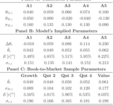
Table 2.2 shows the parameters chosen for assets 1 to 5, that respectively mimic the lowest

to highest book-to-market quintile portfolios. Asset 1 (A1), that resembles the growth portfolio,

has the lowest state-shift risk among the assets, ∆θ1 =−0.01, the lowest unconditional drift,

¯

θ1 = 0.04, and the largest volatility σ1 = 0.16. On the other side is asset 5 (A5), that resembles the value portfolio. It has the highest state-shift risk, ∆θ5 = 0.23, but also the highest unconditional drift θ¯5 = 0.062 and the lowest volatility, σ5 = 0.09. Note that this diﬀusion term is smaller than the one implied by the data. This was needed to match sample

and theoretical returns, a result of our calibration strategy discussed above10_{. The correlation}

parameters, ρij, were set equal to 0.25, 0.15, 0.10 and 0.05 for |i−j| equal to 1, 2, 3 and

4, respectively, and sets a higher correlation to portfolios with similar book-to-market values.

Table 2.2 also shows the expected excess returns and deviations at πt = πs implied by the model, i.e. the unconditional moments, as well as the sample counterparts of the ﬁve

book-to-market portfolios11. A comparison of the values on Panel B and Panel C shows that the model

reproduces the cross-section dispersion on expected returns of the book-to-market portfolios

10_{If we imposed a higher variance for A5 cash-flow and kept the state-risk spread, this would have resulted in}

a very risky asset with an incompatible high expected returns. We preferred to keep the state-risk spread but reduce the diffusion risk.

11_{Cash-flow levels are set at 1. At this point, the drift parameters better approximate the log-dividend changes}

(27)

for reasonable parameters.

2.3.2 Conditional Betas

Given the parameters that calibrated the model, functions f and S can be computed

numeri-cally and the pricing formulas in equation (4) follows. Next, we discuss the properties of these

formulas. First, we discuss how conditional betas diﬀer across asset for given levels of beliefs.

Then, we discuss how conditional betas diﬀer across assets given changes in investor beliefs,

that is, following the arrival of news.

2.3.2.1 Cross-Section Asymmetries

Figure 2.1 shows the model’s main expressions for all possible values ofπtand fixed cash-flows at Dt= 1. On the top-left plot, we see that A1 has the highest price on almost all the domain of πt. This asset is the least profitable, as it has the lowest unconditional drift among all cash-flows, but also the least susceptible to changes in the economic conditions and so less

risky. At the other extreme is asset A5, which is the most proﬁtable one, but also the most

risky and discounted one, with the lowest price on almost all the domain ofπt. In the top-right plot we see that expected returns for asset A5 is the most sensitive to πt, changing from 3%, whenπtis close to one, to almost15%, when uncertainty is higher. All the other cyclical assets also have increasing expected returns on uncertainty, but the change is less substantial. The

expected return on the countercyclical asset A1 slightly declines on uncertainty. The second

row in Figure 2.1 shows covariances of the assets with the market as well as the variances of

asset returns. The shapes are similar to the ones implied by the risk-neutral case, but peaking

slightly to the right of the maximum uncertainty point, aroundπt= 0.6.

The last four plots in Figure 2.1 show all the elements in the factor decomposition of excess

returns (5), the market betas, βim,t, hedging betas,βiπ,t, and their corresponding prices, λm,t and λπ,t, as functions of all possible values of πt and given cash-ﬂows. First, we observe that the premium for exposure to market risk is more important than the premium for exposure

to hedging risk. The most sensitive asset to the hedging factor, A5, has the highest absolute

(28)

that the market portfolio is likely the most important factor determining expected returns and

justiﬁes the assumption made by Jagannathan and Wang (1996) of hedging motives not being

suﬃciently important.

Second, as we previously noted analytically for the risk-neutral case, market beta of assets

with a high and positive ∆θi, such as A5, increases as uncertainty about the state of the economy increases. Since the investor is now risk-averse, the market beta of asset A5 peaks

slightly above12 the point of maximum uncertainty, taking its maximum value ofβ5m,t = 1.80 at around πt= 0.60. On the other hand, the beta of asset A1, declines as πt moves away from

0 and 1, reaching a minimum of β1m,t = 0.40 also aroundπt= 0.60. We note also that there is enough variation in betas to make A1 riskier than A5. In periods of low uncertainty, e.g.

whenπt>0.95, the beta of A1 is higher than that of A5.

Third, the price of market risk, or the market premium, is positive and also increasing

on uncertainty. It reaches a maximum of about λmt = 8% at πt = 0.60 and a minimum of

λmt= 3%atπt= 1. Atπs= 0.83, the unconditional or long run mean of the random variable

πt, the price of market risk is6.5% and close to its historical sample mean13.

Finally, time-variation of market betas is relevant to some assets but less important to

others. Figure 2.1 indicates that for A1 and A5, both the conditional market beta and price

of market risk are equally important for the asset’s risk premium. Consider a shift to investor

beliefs from π1 = 0.90 to π2 = 0.50. The price of market risk, λmt, increases from 4.93% to

7.81%, a change of 58%. Likewise, asset A5 beta also change signiﬁcantly, from 1.33 to 1.87,

an increase of 41%. The change in the asset A1 beta is also important but to the opposite

direction, from 0.72 to 0.42, a decrease of 42%. The variation in the betas is less important

than the variation in the price of market risk for the other assets, as we clearly observe from

the plots.

The above expressions are for all possible values of πt ∈ [0,1], but not all are equally likely. For the chosen parametrization, in particularly λandµthat matches the U.S. business

12_{This rightward shift resulting from increases in risk aversion was also observed, in the single asset case, by}

Veronesi (1999).

(29)

cycles, most of the mass of theπtdistribution is above0.50, since the economy is most often in expansionary periods. Thus, on average, negative news about the economic conditions increases

uncertainty while positive news decreases it. Consequently, the response of market betas14 to

news is asymmetric due its (approximately) monotonic relation to uncertainty.

Another aspect of the πt distribution under this parametrization is that periods of higher uncertainty most often occur during the bad state. The persistence of learning process coupled

with its shorter duration results in a higher proportion of uncertainty periods during the bad

state. Therefore, volatility of asset returns, the covariance of cyclical asset with the market

returns and the price of market risk, will tend to be higher during the bad state, as these

vari-ables typically increase on uncertainty. The model thus provides theoretical justiﬁcation to the

empirical ﬁndings that such variables tend to increase during recessions. Another implication

of the model is that the value premium should be higher during the bad state, as the diﬀerence

in market betas of value and growth portfolios is also higher during high-uncertainty periods.

This countercyclicality of the value premium predicted by the model has also been observed

empirically (Petkova and Zhang, 2005).

2.3.2.2 Time-Series Asymmetries

To assess the relevant portion of the pricing formulas, we generate time-series of the variables

in our model using the same parameters discussed in the calibration. Once cash-ﬂows are

gen-erated according to (2.1), beliefs are computed as indicated by the optimal ﬁltration equation

(1). These state variables,πtandDt, are then used to determine the model’s pricing formulas. The length of the generated series is equivalent to a sample of six years of daily data. We avoid

a sample larger than 6 years because of our assumption that cash-ﬂows follow an arithmetic

Brownian motion. As the cash-ﬂow level moves away from its starting value, D0 = 1, the drift of the stochastic process becomes a worse approximation of percentage changes, the scale

used for the calibration. On the other hand, we do not select a smaller sample because of the

duration of recessions and expansions implied by the transition matrix parameters. The six

year time frame allows an expansionary period lasting ﬁve years and a recession lasting one

(30)

year, which implies average durations and proportions of good and bad months that are similar

to the ones imposed by the calibration of λand µ.

In order to assess how the proportion of good and bad states can have an impact, we

consider three diﬀerent combinations of good and bad states. First, we consider the case of

no bad state and six years of good state. We will refer this case as the bull market case. In

the second scenario the economic conditions are average, with ﬁve years of the good state and

one year of the bad state. In the third scenario, two out of the six years the economy is in

the bad state. We refer this as the bear market case. For all three scenarios, the bull, bear

and regular markets, 500 histories are generated, each with 1584 observation (six years of daily

observations).

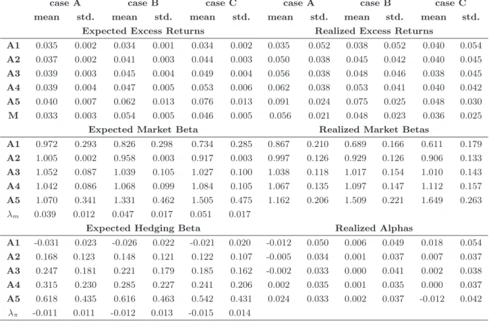
The top two panels in Table 2.3 show the averages and standard deviations across the 500

histories of the expected and realized excess returns. We observe that for the bull and bear

markets, expected excess returns do not coincide with realized excess returns. In the bull

market case, asset A5, that resembles the value portfolio, outperforms and has higher realized

returns than would be expected; the annual average realized return of asset A5 is around 9%

and the average annual expected returns is 4%. On the other hand, in the bear market, A5

underperforms, with an annual average realized return of 4.8% against an average expected

return of7.6%. The opposite holds for asset A1, the asset that resembles the growth portfolio.

It underperforms in the bull market but overperforms in bear market. When the economic

conditions are the ones implied by the calibration, the second scenario, expected returns are

similar to the realized ones. The values do not coincide because of sample variation and

of the approximation imposed by the assumption that cash-ﬂows follow arithmetic Brownian

motions15.

Since expected excess returns also have a factor characterization in our model, such

dis-crepancies or anomalies observed above for expected returns are also observed in the factor

regression. The pricing errors captured by the intercepts of static CAPM regressions, the

real-ized alphas in the lower-left panel of Table 2.3, indicates the existence of a value premium when

15_{Veronesi (2004), that investigates the properties of the univariate version of our model, also faces similar}

(31)

sample are generated by bull markets. The average intercept across all histories is negative for

asset A1 and positive for asset A5. The opposite is observed for bear markets, where a growth

premium arises. We have deliberately ignored the hedging factor in the regressions of the static

CAPM, as its contribution to risk premium is much smaller than the exposure to market risk.

As Table 2.3 shows, the average price of the hedging risk is aroundλπ =−1%and the average quantity of hedging risk is 0.6 for the asset A5, resulting in an average hedging premium of

about ₋0.6%, less than a tenth of the market risk premium,6.5%.

These results point to an interpretation of the forces behind the value premium related to

biased sampling. A similar argument has been employed by Veronesi (2004) to explain the

equity premium puzzle. The author, using the univariate version of our model, attributes the

apparent puzzle that market average returns are too high relatively to its observed (realized)

riskiness, to a rational premium required by the investor to account for a peso-problem type of

event – a very unfavorable event, which the investor is aware of, that has never happened, at

least in the particular sample considered.

The importance of the sample to the value premium was also observed by Ang and Chen

(2007). They argue that most studies that ﬁnd a value premium on the U.S. stock market

generally consider only the post-1963 period, mainly due to the ready availability of data, and

that the omission of previous years is key to ﬁnding a value premium. In fact, they show

that the alphas in the static CAPM regressions turn out to be insigniﬁcant when the sample

is extended to include the months from 1926 to 1962. Since our objective is to explore the

dynamics of market betas implied by our theory and not to propose a solution to the value

premium, we restrict our analysis to the unbiased histories generated under the second scenario.

For the task of unveiling the dynamics of market betas, we ﬁrst ﬁt an univariate asymmetric

GARCH(1,1) model to the simulated returns to discuss the dynamics of volatility. The

speciﬁ-cation of conditional volatility, also referred to as GJR-GARCH model (Glosten, Jagannathan,

and Runkle, 1993), is the following:

rit = αi+uit

(32)

where uit = σitǫit, ǫit iid∼ N(0,1), and 1[.] the indicator function. This speciﬁcation is ap-propriate here as it allows past shocks to inﬂuence future volatility, in line with the model

assumption that investor beliefs are based on past information, and also because the sign of

shocks, consistent with the learning feature of the model, can be informative about shifts in

the economic conditions.

We use mean-adjusted past excess returns as proxies for cash-ﬂows news, which is what

actually drives beliefs. This can be justiﬁed by the following. From equations (1) and (4) we

observe that both beliefs and excess returns are driven by same the standard Brownian motion,

dvt. Furthermore, both diﬀusion terms in those equation, σπ and σiR, indicate that shocks to returns will be positively related to shocks to beliefs when the term S_i′(πt) +pπi is positive, which is the case for all cyclical assets on most values of πt (the term Si′(πt) can be negative and oﬀset pπi for lower values ofπt, which only seldom occur).

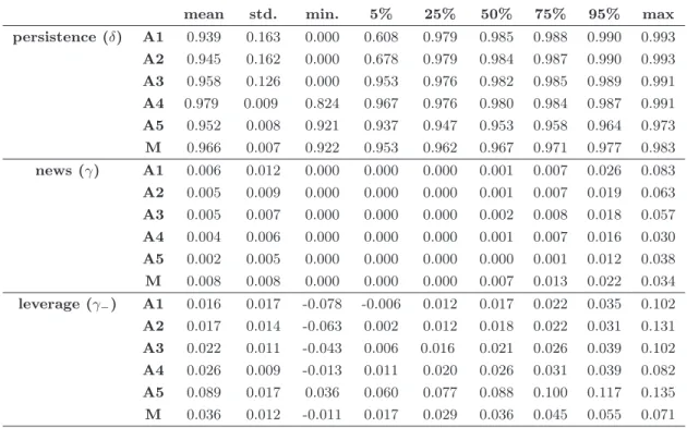
Table 2.4 shows the averages, standard deviations and quantiles of the estimated parameters

of (2.10) across the500histories for each asset. First, we observe that conditional volatilities are

very persistent, theδ’s are high and close to one, a well known stylized fact about stock returns.

Second, negative shocks to returns are more important to future volatility than positive shocks,

as for all assets the coeﬃcient γ− is positive. This asymmetric response of volatility to past

shocks has long been observed empirically and referred to as the leverage eﬀect (Black, 1976).

Finally, assets with cash-ﬂows that are more exposed to shifts have stronger asymmetries. The

average coeﬃcient γ− across the 500 histories for asset A5 is 0.089 while for asset A1 it is

only0.016. This was expected, as A5’s expected returns is the most responsive one to changes

in uncertainty. Furthermore, shocks to A5 are also the most informative ones, as it has the

highest signal to noise ratio among all cash-ﬂows.

We now turn to the question of how the covariances respond to past shocks. In order to do

so, we ﬁt an asymmetric multivariate GARCH model to the simulated data. More precisely,

we follow the BEKK speciﬁcation of Engle and Kroner (1995) but also introduce asymmetric

terms as in Hafner and Herwartz (1998). For computational convenience, we focus on bivariate

models of asset excess returns and market excess returns.

(33)

portfolio, the vector as ut = [uit, umt]′ and let Gt be the information set at time t. The conditional joint distribution is assumed to beut|Gt−1∼!0,Σt|t−1

with conditional covariance

given by

Σt|t−1 = C′C+A′Σt−1|t−2A+B′ut−1u′t−1B (2.11)

+1_[u_it₋₁_<0]D′₁ut−1u′t−1D1+ 1[umt−1<0]D

′

2ut−1u′t−1D2

whereA,B,D1 andD2 are 2×2matrices and C an upper triangular2×2 matrix. Matrices

D1andD2 are new to the original BEKK formulation and add the needed ﬂexibility to capture asymmetric responses of the covariance matrix to shocks. Assuming that the joint distribution

is normal, parameters are estimated by maximizing the log-likelihood function.

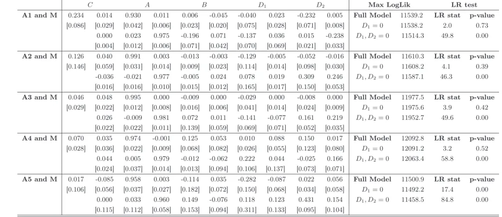
The estimated parameters16of equation (2.11) for a simulated17history are shown in Table

2.5. We also show the log-likelihood ratio (LR) statistics that compares the full model (2.11)

with an speciﬁcation with just one asymmetric matrix, D2, and another with no asymmetric matrices. The LR-test p-values indicates that the diﬀerence in the likelihoods of the symmetric

BEKK and the asymmetric BEKK, with matricesD1 andD2, are statistically signiﬁcant. The LR-test also shows that asymmetries at the asset level are not statistically relevant, except for

asset A5. This was expected, as A5 is the most informative asset about the state of the nature

and so its returns shocks relate more closely to changes in aggregate returns.

We can also see that asymmetries are relevant by noting that the parameters on matricesD1 andD2 are signiﬁcant and relatively large. However, in order to make sense of these numbers, we compute impulse response functions (IRFs). First, we need to rewrite the matrices of

parameters in vector form using the vec operator that stacks columns:

vec(Σt) = C+Avec(Σt−1) +Bvec

! utu′t

+D11[uit−1<0]vec !

utu′t

+D21[umt−1<0]vec

! utu′t

16_{The asymptotic distribution of the estimates is generally unknown and the results can only provide a}

description of the dataset (Herwartz and Lutkepohl, 2000).

17_{The precise results can vary, depending on the particular history chosen. We have selected the history}

(34)

whereC= (C_⊗C)′vec(I2),A= (A⊗A)′,B = (B⊗B)′,D1= (D1⊗D1)′,D2 = (D2⊗D2)′ andI2is a(2×2)identity matrix. Here,vec(Σt)will then be a(4×1)vector, with the ﬁrst ele-ment being the asset return conditional variance, the second and third eleele-ments the conditional

covariance of the asset return with the market return and the last term the market return

con-ditional variance. Hafner and Herwartz (1998) deﬁne the IRF as Vt(ξ0) =E[vec(Σt)|ξ0,Σ0], which can be computed by starting the above auto-regression at the long run value of the

covariance matrix,Σ, and perturbing it with standardized shocks,ξ0. Att= 1 we have

V1(ξ0) = C+

B+ 1_[ξ0_,i_<0]D1+ 1[ξ0,m<0]D2

vecΣ1/2ξ0ξ′0Σ1/2

+Avec(Σ)

and for t_≥2

Vt(ξ0) = C+

A+B+D1

2 +

D2

2

Vt−1(ξ0)

Impulse response functions for betas easily follow from the ratio of the covariance and

market variance IRFs:

βit(ξ0) =

Vim,t(ξ0)

Vm,t(ξ0)

whereVim,t(ξ0) and Vm,t(ξ0) are the second and fourth elements of the vectorVt(ξ0).

Figure 2.2 shows the IRFs of assets A1 and A5 22 days after the initial shock. The ﬁrst

column shows the variances IRFs. The upper plot shows the responses to shocks in the market

portfolio, leaving asset return unperturbed, and the lower plot responses to shocks in the assets,

leaving market return unperturbed. The asymmetric response to shocks is clear, particularly to

A5, as was noted in the univariate estimation above. We observe that negative shocks to both

market and the assets returns result in a larger change in the volatility than positive shocks.

The second column in Figure 2.2 shows the IRFs of the covariance of assets A1 and A5

with the market portfolio, where we have written the y-axis in terms of percentage changes

to the initial position. The upper plot shows how shocks to the market portfolio changes

(35)

the covariance of A5 with the market portfolio substantially. On the other hand, when the

shocks are positive, the covariance declines slightly. This shape is in line with our previous

discussion on the relation of covariances with uncertainty and how uncertainty changes with

news. The covariance of A1 with the market portfolio is relatively stable, and slightly increases

with negative shocks and slightly decreases after positive shocks in the market portfolio. The

lower plot on the second column, shows a similar response of the covariance of A5 to shocks on

its own returns, but with changes of smaller magnitude.

Finally, the last column in Figure 2.2 shows the betas IRF for both assets A1 and A5. In

the top plot we see how betas respond to shocks in the market. As discussed analytically, we

have that negative shocks to market returns result in an increase in the market beta of the

asset A5 but a decrease in the market betas of A1. A5 beta increases by about 30% on large

negative news, while A1 beta decreases by about 30% on large negative news. On the other

hand, positive news have a much smaller impact on betas.

2.4 Conclusion

The implications of the model for the variance, covariance and conditional market betas of

asset returns conﬁrm many empirical facts and also suggests new results. First, as pointed by

Veronesi (1999) for the market portfolio in the univariate model, excess returns display the

predicted volatility asymmetry so pervasive in real data. This has been originally attributed

by Black (1976) to a leverage eﬀect, but in our model the justiﬁcation is closer to the volatility

feedback hypothesis of Campbell and Hentschel (1992). A novel implication for the dynamics

of volatility is that assets that are very sensitive to the economic conditions should also display

stronger asymmetric responses to news.

Second, the covariance of asset returns with the market portfolio also responds

asymmet-rically to the arrival of news, a result also veriﬁed empiasymmet-rically, for instance, in the contagion

literature of international markets (Ribeiro and Veronesi, 2002). Our model shows that

neg-ative news increases the covariance of cyclical assets with the market portfolio by a larger

magnitude than positive news. Again, this asymmetry will be larger the more sensitive the

(36)

predicts an opposite asymmetric response of covariances to news.

Third, the conditional market betas respond asymmetrically to news. Market betas of assets

that are very sensitive to changes in the economic conditions increase during high uncertainty

cases as opposed to less sensitive assets. A concrete example of assets with such opposing risk

dynamics, as shown in the calibration exercise, are the value and growth portfolios.

The empirical evidence regarding the asymmetric response of market betas to news is

unclear (Braun, Nelson, and Sunier, 1995). Nonetheless, the diﬃculty of assessing the opposite

response of betas to news from realized returns in a multivariate GARCH framework was also

present in our investigation under the controlled environment of simulated returns. Despite the

analytical equations indicating that asymmetries are relevant, the parameters estimated from

an asymmetric GARCH model did show such asymmetries but for some histories only. Since

the forces behind the beta asymmetry are the same ones behind the asymmetry of variance and

covariances, which are two well known empirical facts about stock returns, the lack of empirical

evidence of beta asymmetry could be a result of econometric misspeciﬁcation as opposed to

4741.pdf

Conditional Betas: Asymmetric Responses to Good and Bad

News

Abstract

Acknowledgments

Contents

List of Tables

List of Figures

Chapter 1

Introduction

Chapter 2

Theoretical Model

2.1

Introduction

2.2

The Model

2.3

Simulated Economy

2.4

Conclusion