Abstract
Susan Michele Teefy. Performance and Analysis of Tracer Studies
to Determine Compliance with the Disinfection Requirements of the
Surface Water Treatment Rule, (under the direction of Philip C.
Singer)
The Surface Water Treatment Rule includes disinfection
requirement which will apply to all water systems using surface
water sources. One objective of this project was to conduct tracer studies at selected water treatment plants in order to determine the residence time distributions of various process
units. The plants were evaluated to determine whether they will
be able to comply with the disinfection requirements of the Surface Water Treatment Rule. CT's, the Concentration of
disinfectant multiplied by the Time it is in contact with the
water, were determined for each plant under different conditions.
These were compared to CT values supplied by the Environmental
Protection Agency for specific degrees of pathogen inactivation.
A second objective was to develop a more precise method for estimating the CT. This theoretical construct, the "effective CT", made use of the residence time distributions and the kinetics of chlorine decay to more accurately predict the degree ofpathogen inactivation as expressed by the chlorine concentration
multiplied by the contact time. All three of plants studied will
be able to meet the disinfection requirements of the Rule. As
demonstrated by comparing the "effective CT's" to the CT's allowed
by the Surface Water Treatment Rule, a substantial margin of
safety is implied in the degree of inactivation allowed by the
Rule. Problems were discovered with using fluoride as a tracer in
the presence of aluminum hydroxide; sodium was demonstrated to be
Performance and analysis of tracer Studies to determine Compliance with the
Disinfection Requirements of the Surface water treatment rule
TABi.F. OF Contents
Abstract... ii List of figures...iv List of tables...vi 1.0. Introduction... 1-1
2 . 0 Background and Theoretical Concepts... 2-1 2.1 Drinking water and health... 2-1
2 .2 Surface Water Treatment Rule... 2-6
2.3 The CT concept for inactivation... 2-8
2.4 Determination of "C" and "T"... 2-10
2.5 Chemical reactor theory and flow models...2-14 2.6 Kinetics of chlorine decay and pathogen
inactivation...2-19 3.0. Experimental Methods... 3-1 3 .1 Description of Plants... 3-1 3.1.1 WSSC Patuxent Filtration Plant...3-2 3.1.2 WSSC Potomac Filtration Plant...3-4 3.1.3 OWASA Filtration Plant...3-6 3.2 Experimental and Analytical Methods... 3-8 3.2.1 Step-input tests...3-9 3.2.2 Pulse-input tests...3-12 3.2.3 Fluoride analysis...3-15 3.2.4 Sodium analysis...3-16 3.2.5 Analysis of data...3-18 4 .0 Results and Discussion... 4-1 4 .1 Step-Input Tests... 4-1 4.1.1 Potomac filtration plant results...4-1 4.1.2 Patuxent filtration plant results...4-7 4 .2 Pulse-Input Tests... 4-12 4.2.1 Patuxent filtration plant results...4-13 4.2.2 OWASA filtration plant results...4-20 5 .0 Summary and Recommendations... 5-1
References
Appendix I: CT Tables from Guidance Manual for Compliance with the
Filtration and Disinfection Requirements for Public Water Systems
Using Surface Water Sources, March 31, 1989Appendix II: Protocol for Conducting Tracer Tests at the Patuxent
Filtration Plant
T.TST OF FTCURKS
Figure Page Number
2-1 Effect of water treatment on waterborne disease
death rates... 2-la
2-2 Schematic of ideal reactors... 2-14a
2-3 Pulse and step input response, PFR, CSTR...2-15a 2-4 Residence Time Distribution Curve (E curve)... 2-16a 2-5 F curve... 2-16b
2-6 Tanks-in-series model response to tracer test...2-17a 2-7 Plug flow with dispersion model ... 2-19a 3-1 Flow diagram of the Patuxent filtration plant...3-2a 3-2 Schematic plan view of the Patuxent filtration plant. 3-3a 3-3 Flow diagram of the Potomac filtration plant...3-5a 3-4 Schematic plan view of the Potomac filtration plant.. 3-5b 3-5 Flow diagram of the OWASA Filtration Plant...3-7a 3-6 Schematic plan view of the OWASA filtration plant.... 3-7b 3-7 Diagram of influent and effluent structures at
Potomac plant... 3-lla 3-8 Typical Fluoride standard curve... 3-16a 3-9 Typical Sodium standard curve... 3-18a
3-10 F curve from a step-input test with Tio
determination... 3-19a
3-11 F curve and corresponding E curve... 3-19b 3-12 Pulse-input test and corresponding F curve...3-20a 3-13 Pulse-input test and corresponding E curve...3-21a
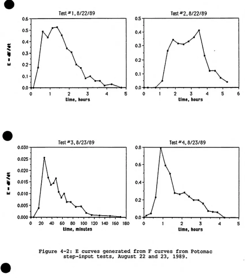
4-1 Step-input tests, Potomac filtration plant,
8/22-23/89... 4-2a 4-2 E curves from F curves, Potomac filtration plant...4-4a
4-3 Tanks-in-series model fitted to Potomac data...4-5b
4-4 Flow chart from Patuxent plant, 5/18/89... 4-7a 4-5 Step-input tests, Patuxent filtration plant,
5/15-18/89... 4-8a 4-6 E curves from F curves, Patuxent filtration plant....4-lOa 4-7 Ideal CSTR model fitted to Patuxent data... 4-llb 4-8 Pulse-input tests, Patuxent plant, 5/19/89...4-13a 4-9 Pulse-input test #2, Patuxent plant, 8/24/89... 4-15a 4-10 Pulse-input test #3 (using Sodium) at Patuxent,
10/12/89... 4-16a 4-11 Comparison of E curves for Na and fluoride tests,
Patuxent... 4-17a 4-12 Tanks-in-series model fitted to Patuxent
sodium test data... 4-20a 4-13 Pulse-input test with F curve, OWASA clearwell,
9/24/89... 4-21a 4-14 Tanks-in-series model fitted to OWASA clearwell
test, 9/24/89... 4-22a 4-15 Pulse-input test through OWASA filter, entire
plant, 8/15/89... 4-24a
#
Figure P&qe Nunfeec
4-17 Pulse-input through OWASA filters using NaF,
9/21/89... 4-25a
4-18 Comparison of Na and F pulse input, OWASA filter,
9/15/89... 4-25b
4-19 E curves for Na and F pulse input, OWASA filter,
9/15/89... 4-25C
4-20 F Curve for OWASA filter from Na pulse input,
9/21/89... 4-26a
4-21 Tanks-in-series model fitted to F curve for OWASAT.TST OF TABLES
Table Page Number 2-1 Waterborne disease occurrence in the United States,
1971 to 1981... 2-2a 2-2 Expected fiiardi a and virus removal rates for
different filtration technologies... 2-7a 2-3 Example CT values from Guidance Manual... 2-9a
4-1 Sample calculations for step-input test,
Potomac Test #1... 4-2b 4-2 Tio and T50 values for step-input tests,
Potomac plant... 4-3a 4-3 Mean residence times for Potomac step-input tests..., 4-4b 4-4 CT values for step-input tests, Potomac plant... 4-5a
4-5 Tio and T50 values for step-input tests,
Patuxent plant...ͣ. 4-8b
4-6 Mean residence times for Patuxent step-input tests.. 4-lOb 4-7 CT values for step-input tests, Patuxent plant... 4-lla
4-8 Sample calculations for pulse-input tests,
Patuxent test... 4-16b
4-9 Summary of pulse-input test results, Patuxent... 4-18a 4-10 Summary of pulse-input test results, OWASA
l.Q INTRODUCTION
The primary purpose of drinking water treatment is to render the water safe to drink. Diseases such as typhoid and cholera can spread quickly through a population which is exposed to a
contaminated water supply. Indeed, such waterborne disease
outbreaks were common around the turn of the century before water treatment was universally practiced. Treatment for the prevention of waterborne disease initially consisted of disinfection; later, filtration was added as another barrier to pathogenic
contamination. Because of the widespread use.of chlorine as a disinfectant, waterborne disease outbreaks in the United States dropped dramatically, and today such outbreaks are rare.
Recently, a protozoan cyst, Giardia lambXig/ has become a concern to the water supply industry because this microorganism is more resistant to chlorination than most waterborne bacteria. It has been detected in water supplies and has been implicated in outbreaks of giardiasis, a type of gastroenteritis. Although it is not easily inactivated with chlorine, Giardia can be removed
with proper filtration.
Over the last fifteen years, chlorine has been shown to combine with naturally occurring organic matter in water to produce by-products which are thought to be carcinogenic. This
information has caused the water industry to reconsider current methods of disinfection given competing objectives: disinfect the
•
water to such a degree that pathogens are inactivated, but do not add so much disinfectant that harmful by-products are formed.
In order to ensure that all water supplied to the public in the United States meets certain standards for quality. Congress
passed the Safe Drinking Water Act in 1974. This Act includes a
list of standards which all drinking water supplied to the public
must meet. The SDWA was amended in 1986, and the number of
standards which water suppliers must meet increased almost four¬ fold. The 1986 amendments also stipulated that all surface water
supplied to the public must be filtered and disinfected. This was
done mainly because of concern over the occurrence of GiardiaIambila cysts. In response to the SDWA amendments, the Environmental Protection Agency developed the Surface Water
Treatment Rule. This is a set of specific criteria which apply to
all surface water systems.
According to the Surface Water Treatment Rule, water systems
must demonstrate that they can achieve a 99.9% (3-log) reductionin the number of viable Giardia cysts and a 99.99% (4-log)
reduction in the number of viable enteric viruses in the finished
water. Rather than monitoring the raw and treated water for these
microorganisms, the SWTR contains a series of filtration andWater systems can meet the required degrees of
removal/inactivation by filtration and disinfection, or in some cases, by disinfection alone. Depending on the type of filtration used and the way in which the filters are operated, the regulatory agency will give a certain removal "credit" to each surface water system, usually between 2-log and 3-log (99% and 99.9%) removal credit for Giardia cysts. The remainder of the
removal/inactivation (1-log to 2-log, 90% to 99%) must be achieved through disinfection.
In order to demonstrate that a particular disinfection scheme achieves the required degree of inactivation, CT products are
used. CT is the product of the Concentration of the disinfectant, in mg/1, and the Time, in minutes, that the disinfectant is in
contact with the water. The SWTR contains tables of CT values
that have been demonstrated to achieve specific degrees of inactivation for various water quality conditions. If the CT product for a water treatment plant meets or exceeds those
published in the SWTR tables, then it is assumed that the degree of inactivation has been achieved. Each plant's compliance status depends on this demonstration. Therefore, the methods by which the values for "C" and "T" are calculated are very important.
The value used in the SWTR for C is the residual disinfectant concentration at the effluent of the process unit in question. In the case of chlorine, this approach does not take into account the fact that chlorine is relatively reactive, and dissipates
continuously throughout the reactor as it is consumed by
contaminants in the water. If the oxidant demand of the water is
high, a much higher dose of chlorine may have been added at the
influent to the reactor than was detected at the effluent. This
means that some elements of the fluid were exposed to a higher concentration of chlorine than others, although for a shorter time, while other elements of the fluid were exposed to the effluent concentration. These variations in chlorine
concentration and exposure are not accounted for in the SWTR
calculations.
For pipelines, the value used for T in the SWTR is the theoretical detention time, which is the volume of the pipe
divided by the flow rate. For mixing basins, storage reservoirs, and other units, tracer tests must be conducted. In this case, the value used for T in the calculation of the CT product is Tio, the time it takes 10% of the mass of the tracer to pass through the vessel. This is a somewhat arbitrary definition of T. Other, better defined, methods are available for characterizing the flow through process units. The unit can be assumed to behave as an
ideal reactor, or one of several non-ideal flow models can be
used. Residence Time Distributions, or E curves, can be developed
to more precisely define and characterize the behavior of the
Tio-The objectives of this project were as follows: first,
conduct tracer studies at several selected full-scale water
treatment plants and determine Tjq values for the various process units exposed to the disinfectants. Second, calculate the CT
allowed by the SWTR for each water system, and compare these to the required CT values to determine if the plants are in
compliance with the SWTR disinfection requirements. Third, develop Residence Time Distributions (RTDs) for the various
process units at each plant and calculate the effective or actual CT, based on the RTD and the kinetics of chlorine decay, and
compare these to the CT allowed by the SWTR.
Three full-scale water treatment plants using surface water
sources were evaluated. These were the Potomac Filtration Plant
and the Patuxent Filtration Plant of the Washington Suburban Sanitary Commission, located in Laurel and Potomac Maryland; and the Orange Water and Sewer Authority Filtration Plant in Carrboro, North Carolina. Tracer tests were conducted using both the step-input method and the pulse-step-input method. Fluoride was the primary
tracer chemical.
2.0 BACKGROUND AND THEORETICAL CONCEPTS
2.1 Drinking Water and Health
The connection between treatment of drinking water and
public health is well established in the United States. Prior to
the introduction of chlorine as a water disinfectant in 1908 and its subsequent widespread use throughout the country, waterborne diseases (caused by consumption of water containing pathogenic microorganisms) such as cholera and typhoid fever were prevalent. At the turn of the present century, the death rate from typhoid
fever averaged 30 per 100,000 in U. S. communities (1). After the introduction of chlorine compounds as water disinfectants, the incidence of typhoid was substantially decreased, eventually to less than 0.1 per 100,000 (1). Other diseases, such as
gastroenteritis, dysentery, and hepatitis, can also be waterborne. While these are not as likely to be fatal as typhoid or cholera, they can cause prolonged illness and severe discomfort (2).
Figure 2-1 is an example of the dramatic decline in waterborne disease fatalities in two typical cities: Pittsburgh, Pennsylvania and Detroit, Michigan, since their water supplies have been
treated (1).
Treatment of drinking water from about 1910 until about 1970 focused on removing or killing pathogens in order to prevent
waterborne diseases. The most common form of treatment was the
addition of chlorine to such a level that bacteriological tests
indicated that the water was "safe". The indicator that has been350
8 o g
Annual values
Diarrhea and
enteritis Typhoid
Untreated Filtered Filtered and chlorinated
Annual
values
^wm-m.
Untreated Chlorinated Filtered and chlorinated
Figure 2-1: Effect of drinking water treatment on waterborne disease fatalities in the cities of Pittsburgh, Pennsylvania
(top) and Detroit Michigan (bottom) (1)
bacteria. Coliform bacteria are present in large numbers in human and animal wastes. Coliforms themselves are not disease-causing, but their presence is a sign that the water may contain fecal matter and, therefore, pathogenic microorganisms. If the water was free of coliforms, then it was assumed to be free of human
pathogens. Mainly through the use of chlorination, the number of
waterborne disease outbreaks in the U.S. has been greatly reduced.Even though the incidence of waterborne disease outbreaks has been greatly reduced since the turn of the century, such outbreaks
still occur. Table 2-1 summarizes the Environmental Protection
Agency's estimates of the numbers and types of waterborne disease outbreaks in the U.S. between 1971 and 1981 (3). The reported disease incidents probably substantially underestimates the actual occurrence of waterborne disease. Many outbreaks, perhaps the great majority, are not reported (4).
Most recent waterborne disease outbreaks have been attributed
to deficiencies in treatment in water systems using surface water
sources. From 1971 to 1985, the Centers for Disease Control
reported 106 outbreaks of waterborne diseases, involving over
34,000 individuals, attributed directly to public water systems
using surface water supplies (4). All surface water supplies are
at risk from pathogenic contamination, while most groundwater
supplies are not. Most microorganisms are removed fromTable 2-1: Waterborne Disease Outbreaks
in the United States, 1971-1981 (3)
Disease
Gastroenteritis Giardiasis
Shigellosis
Salmonellosis
Hepatitis A
Campylobacter diarrhea Viral gasteroenteritis
vibrio cholerae
Rotavirus
TOTALS: 307 75,596
Outbceaks. Individuals.
192 39,845
50 19,863
25 5,448
8 1,150
16 463
4 3,902
10 3,147
1 17
1 1,761
#
waterborne disease outbreaks, surface water must be treated to a
higher degree than groundwater. In general, surface water systems
using multiple barriers of treatment (i.e., at least filtration
and disinfection) are significantly more effective in preventing
waterborne disease outbreaks (4).
Recently, a particular protozoan microorganism has been
implicated as a major cause of waterborne disease outbreaks.
giardla lamblia has been detected in both raw and treated water
supplies throughout the U. S., particularly in cooler, mountain
regions. This intestinal parasite can cause giardiasis, a type of
gastroenteritis. From 1951 to 1970, only 12 cases of giardiasis
were reported in the U. S. From 1971 to 1981, 50 outbreaks
involving over 20,000 individuals were reported. While some of
this increase can be attributed to improved reporting and
awareness, the disease is in fact more common because of increased human presence in watershed areas (5).
Giardia lamblia can be introduced into water supplies by
mammals other than humans. An outbreak of giardiasis in Camas,
Washington that infected some 600 people, or 10-15 percent of the
population, was believed to be introduced by beavers (6). Giardia
cysts appear to be continuously present, though at low
concentrations, even in relatively pristine rivers (7).
Giardia cysts are known to be more resistant to disinfection
in cold water (6). It is entirely possible for a water system that is contaminated by Giardia cysts to have no detectable coliform bacteria and still have viable Giardia cysts present. The same is true for enteric viruses, since their presence or absence is not necessarily reflected by coliform tests. Indeed,
documented outbreaks of giardiasis have occurred in water systems which employed chlorination and detected no coliform bacteria in the system (4). Treatment in addition to disinfection, such as
filtration, can be used to combat Giardia. Since the cysts are relatively large (between 7 and 12 micrometers), they can be
removed by filtration (6). Filtration is not effective unless the raw water has been properly conditioned via coagulation and
flocculation to such an extent that small particles can be
removed. In the Rocky Mountain region of the country, it has been common practice to eliminate the addition of coagulating chemicals to low-turbidity surface waters in the winter. This is done
because the raw water turbidity levels already meet drinking water standards, and effective coagulation and flocculation can be
difficult under these conditions. In such areas, giardiasis is
endemic (6).
In order to ensure that water supplied to the public is safe. Congress passed the Safe Drinking Water Act (SDWA) in 1974. The
Act stipulates that all water supplied to the public must meet
certain standards for quality. The SDWA directed the
Environmental Protection Agency (EPA) to develop a list of
contaminants that might be found in water systems and set maximum
#
allowable levels for these contaminants. EPA sets the Maximum Contaminant Levels (MCLs) based on the health effects of each contaminant, as well as on the technology available to detect andremove the contaminant.
In most of the United States, each state enforces the
provisions of the SDWA for the water systems within that state. Each water supplier is responsible for taking samples of the water at regular intervals, seeing that these are properly analyzed, and getting the results to the appropriate regulatory agency. The suppliers of water are subject to enforcement action if they
supply water which does not meet the standards. In this way, the public can be assured that the water they are drinking is safe.
In addition to contaminants which have acute or short-term health effects such as the pathogenic microorganisms discussed above, the SDWA addresses chemicals which have chronic or long-term effects. Compounds which have been found to have chronic effects such as cancer have shifted the emphasis of the water supply industry from prevention of waterborne diseases to removal of these carcinogenic compounds. The technology for detecting these compounds and understanding their health effects has
that it does not cause waterborne diseases, but do not add so much
disinfectant that harmful disinfection by-products are formed.
In 1986, Congress amended the Safe Drinking Water Act. The
amendments directed the EPA to develop additional MCLs, expanding the number of contaminants regulated from 23 to 83. The
Amendments also directed EPA to establish criteria whereby surface
water systems would be required to filter their water, and all
water systems would be required to disinfect their water (8).
These last two requirements may prove to be the most far-reaching
to date, affecting every water system in the country and costing
billions of dollars.
2,2 The Surface Water Treatment Rule
In response to the SWDA Amendments, EPA developed the Surface Water Treatment Rule (SWTR) in June 1989. This rule applies to all public water systems which use surface water as a source of supply. The goal of the SWTR is to control five contaminants: Glardia lamblia. enteric viruses, Legionella, turbidity, and heterotrophic bacteria. Rather than setting an MCL for each of these contaminants, EPA developed treatment requirements to
minimize and control their entry into water distribution systems
(9).
According to the SWTR, each water system that uses surface water must demonstrate that it achieves at least 99.9% (3-log) removal and/or inactivation of Giardia cysts and at least 99.99%
(4-log) removal and/or inactivation of viruses. These levels of
treatment can be achieved by a combination of filtration and disinfection, or by disinfection alone. Water systems usinggroundwater are exempt from the SWTR unless they are shown to be
under the direct influence of surface water (9).
The SWTR specifies filtration technologies which, when
properly operated, will achieve the given removal rates. For
example, conventional treatment, which includes coagulation, flocculation, sedimentation, and filtration, can be expected to achieve between 99% (2-log) and 99.9% (3-log) removal of Giardiacysts. Other filtration technologies include direct filtration
(this is the same as conventional filtration excluding
sedimentation), slow sand filtration, and diatomaceous earth filtration. Table 2-2 shows the range of Giardia and virus
removals that can be expected from each type of filtration (10). Surface water systems can use any of the approved filtration technologies so long as the total removal/inactivation by
filtration and disinfection of Giardia cysts and viruses for the
entire system is 99.9% and 99.99%, respectively. Water systems
with very clean, protected sources of supply may only be required
to disinfect to meet the criteria if they meet other prescribed
requirements such as watershed protection and additionalmonitoring.
Table 2-2: Expected Removal Rates for Different Filtration Technologies
(without disinfection) (10)
log removals
Typp of Filtration
Giardia Removal
virus
Removal
CONVENTIONAL
(coagulation, flocculation,
sedimentation, and filtration)
2-3 1-3
DIRECT
(coagulation, flocculation, and filtration, excluding
sedimentation)
2-3
SLOW SAND 2-3*
(low velocity, usually less than
0.4 m/h, biological process)
DIATOMACEOUS EARTH 2-3*
(precoat cake deposited on septum, continuous body feed)
1-3
1-2
*These technologies generally achieve greater than 3-log
removal.
removal/inactivation. EPA recommends that states give systems
"credit" for 2.5-log removal of Giardia and 2-log removal of
viruses for conventional treatment plants that are optimized for
turbidity removal. The remainder of the treatment requirement is
to be accomplished through disinfection (e.g. the systems would
have to disinfect sufficiently to achieve 68% (0.5-log)
inactivation of Giardia and 2-log inactivation of viruses) (10).
2.3 The CT Concept for Inactivation
In order to demonstrate that a particular disinfection scheme
is achieving the required inactivation rate, it is not necessary
to monitor the raw and treated water for the microorganisms. The
Surface Water Treatment Rule makes use of CT products, which are
the product of the disinfectant Concentration (C) and the Time it
is in contact with the water (T). The SWTR and the accompanying
Guidance Manual contain CT tables for various disinfectants atdifferent pH levels and temperatures. The values in the tables
were generated from a statistical analysis of data for Giardia
cyst inactivation kinetics which used both animal infectivity
studies and excystation studies for Giardia cyst viability (10).
Each water system must demonstrate that the product of its "C" and
"T" is equal to or greater than the level shown in the tables.
Appendix I includes the CT tables published in the Guidance
Manual.
destruction of microorganisms as a first-order reaction with respect to the population of bacteria, as follows:
In -^ = -kt (2-1)
Nowhere N = number of organisms present at time t No = number of organisms present at time zero k = rate constant, time"'^
t = time
Watson (12) later produced an equation from Chick's data which included the concentration of the disinfectant used. This equation is referred to as the Chick^Watson Law:
In -^ = -LC"t (2-2)
Nowhere C = concentration of disinfectant
L = coefficient of specific lethality
n = coefficient of dilution
Usually, n is assumed to be 1.0. Both k and L depend on the disinfectant used, the microorganism of concern, and the pH and temperature of the water. Therefore, for a given set of water quality conditions, the product of C and T determines the degree of inactivation (In N/No) for a specific microorganism and a
specific disinfectant. Table 2-3 lists CT values for inactivation of Giardia using free chlorine for two pH values and two
temperatures. According to this table, for a 0.5-log inactivation
Table 2-3: Selected CT values for Giarriia Inactivation (10)
Disinfectant: Free Chlorine
Temperature: 0.5°C
pH: 6.0
Disinfectant: Free Chlorine
Temperature: 25°C
pH: 6.0
Chlorine Chlorine
Cone. log inactivation Cone. log inactivation
(mo/l)_ 0.5 1.0 _1.5 _ 2.0 _ 2.5 _ 2.Q. (mo/lL 0.5_ 1.0 _ 1.5 _ 2.0 _2.5 _ 3.a
<0.4 23 46 69 91 114 137 <0.4 4 8 12 16 20 24
0.6 24 47 71 94 118 141 0.6 4 8 13 17 21 25
0.8 24 48 73 97 121 145 0.8 4 9 13 17 22 26
1.0 25 49 74 99 123 148 1.0 4 9 13 17 22 26
1.2 25 51 76 101 127 152 1.2 5 9 14 18 23 27
1.4 26 52 78 103 129 155 1.4 5 9 14 18 23 27
1.6 26 52 79 105 131 157 1.6 5 9 14 19 23 28
1.8 27 54 81 108 135 162 1.8 5 10 15 19 24 29
2.0 28 55 83 110 138 165 2.0 5 10 15 19 24 29
2.2 28 56 85 113 141 169 2,2 5 10 15 20 25 30
2.4 29 57 86 115 143 172 2.4 5 10 15 20 25 30
2.6 29 58 88 117 146 175 2.6 5 10 16 21 26 31
2.8 30 59 89 119 148 178 2.8 5 10 16 21 26 31
3.0 30 60 91 121 151 181 3,0 5 11 16 21 27 32
Disinfectant: Free Chlorine
Temperature: 0.5''C
pH: 8.0
Disinfectant: Free Chlorine
Teit^jerature: 25°C
pH: 8.0
Chlorine Chlorine
Cone. log inactivation Cone. log inactivation
(mg/1). 0.5. 1.0 1.5 _ 2.0 _ 2.5 _ 3.0 fin<7/n 0.5 1.0 1.5 _ 2.0 2.5 3.0
<0.4 46 92 139 185 231 227 <0.4 8 17 25 33 42 50
0.6 48 95 143 191 238 286 0.6 9 17 26 34 43 51
0.8 49 98 148 197 246 295 0.8 9 18 27 35 44 53
1.0 51 101 152 203 253 304 1.0 9 18 27 36 45 54
1.2 52 104 157 209 261 313 1.2 9 18 28 37 46 55
1.4 54 107 161 214 268 321 1.4 10 19 29 38 48 57
1.6 55 110 165 219 274 329 1.6 10 19 29 39 48 58
1.8 56 113 169 225 282 338 1.8 10 20 30 40 50 60
2.0 58 115 173 231 288 346 2.0 10 20 31 41 51 61
2.2 59 118 177 235 294 353 2.2 10 21 31 41 52 62
2.4 60 120 181 241 301 361 2.4 11 21 32 42 53 63
2.6 61 123 184 245 307 368 2.6 11 22 33 43 54 65
2.8 63 125 188 250 313 375 2.8 11 22 33 44 55 66
of Glardia by free chlorine at pH = 6.0, a temperature of 0.5°C, and a chlorine concentration of 2.0 mg/1, a CT value of 28 mg/l-min (and thus a contact time of 28/2 or 14 mg/l-minutes) would be
required. If the pH stays at 6.0 but the temperature is raised to 25°C, a CT value of only 5 mg/l-min (and thus a contact time of 5/2 or 2.5 minutes) would be required. CT tables are provided for various pH values, temperatures, disinfectants, disinfectant
concentrations, and microorganisms. Illustrative examples of the tables included in the Guidance Manual are included in Appendix I.
When chlorine is used as the disinfectant in a water system, the CT required to achieve a 3-log inactivation of Giardia cysts is always greater than that required to achieve a 4-log
inactivation of viruses. Thus a water system using chlorine need only be concerned with meeting the Giardia inactivation
requirement since at this level, the virus inactivation requirement will also be met. This is not the case for all
disinfectants, most notably chloramines. However, this report
focuses mainly on the use of chlorine as a disinfectant, so
emphasis will be placed on Giardia inactivation instead of virus
inactivation.
2.4 Determination of C and T
The Surface Water Treatment Rule specifies the way in which the values of C and T are to be determined for each water
treatment system. C is the residual concentration, in mg/1, of the disinfectant at the effluent of the process unit or reaction
chamber in question. For example, it might be the free chlorine residual at the effluent of a clearwell. Any point prior to the first customer can be used for analysis of the disinfectant
residual. When ozone is used as the disinfectant, different
procedures are suggested for determination of C due to its
extremely reactive properties and its mode of application. This
report focuses primarily on the use of chlorine for disinfection.
T is the amount of time, in minutes, that the disinfectant is in contact with the water. This is the time it takes the water,
during peak hourly flow, to move between the point of disinfectant
application to a point where the disinfectant residualconcentration is measured prior to the first customer. For pipelines, T is assumed to be the theoretical detention time,
i.e., the volume of the pipe divided by the flow rate. However, in mixing basins, storage reservoirs, and other treatment plant process units and reaction chambers, T must be determined by
tracer tests or other methods approved by each state. When tracer tests are used, the value chosen for T, referred to as T^o, must be
the time it takes 10% of the tracer to pass through the tank (10).
Ninety percent of the water spends at least this amount of time in
the tank. The value of Tio will always be less than thetheoretical time, and if there is a large amount of short
circuiting through the unit, it may be significantly less.
the Guidance Manual (10) suggests regulatory agencies use standard fractions representing the ratio of Tio to T (T being the
theoretical detention time) for the determination. Tracer studies
conducted by Marske and Boyle (13) and Hudson (14) on chlorine
contact chambers and flocculation-sedimentation basins, respectively, were used as a basis in determining these
representative fractions for various basin configurations. The ratio Tio/T was calculated from the data presented in the studies and compared to the associated hydraulic flow characteristics. Values of Tio/T ranged from 0.3 to 0.7. The results indicated a
correlation between Tio/T and the contact basin baffling
conditions, particularly at the inlet and outlet to the basin. The values of Tiq/T were defined for three levels of baffling conditions rather than for particular types of contact basins. General guidelines were developed relating T^q/T values to the
corresponding baffling conditions.
Three general classifications of baffling conditions — poor, average, and superior — were developed in the Guidance Manual to categorize the results of the tracer studies. The values
associated with each degree of baffling are as follows:
poor: 0.1 - 0.3 unbaffled inlet and outlet, no intra-basin baffling
average: 0.4 - 0.6 intra-basin baffling and either a
baffled inlet or outlet
superior: 0.7 - 0.9 at least baffled inlet and outlet and possibly some intra-basin baffling
The Guidance Manual includes examples of basins which fit into each of these categories. From these examples, an estimate of the
ratio Tio/T can be made.
The relative CT contributions to the overall inactivation in each portion of a system are additive. Disinfectant residuals and contact times can be measured in more than one location, and the sum of the degrees of inactivation is the overall degree of
inactivation for the entire system. For example, consider a system which is required to achieve a 99.9% (3-log) inactivation of Giardia cysts. The total inactivation achieved would be
calculated by ,
1. measuring the disinfectant residual, C, at any number of
locations in the treatment train;
2. determining the travel time, Tio* between the points of disinfectant application and each disinfectant measurement; 3. calculating the CT for each point of residual
measurement, CTcaicr and determining CTgg.g required from
published tables in the Guidance Manual;
4. determining the inactivation ratio, CTcaic/CTgg.g for each
segment; and
5. summing the inactivation ratios for each segment, i.e. CiTi/CTgg.g + C2T2/CT99.9 + ... + CnTn/CTgg.g to determine the
overall inactivation ratio.
2.5. Chemical Reactor Theory and Flow Models
Several different theoretical models can be used to describe
the flow of fluid through a vessel. In many cases, the flow can
be idealized, and simple flow model assumptions can be used. Two
of the simplest and most commonly used are the Continuously
Stirred Tank Reactor (CSTR) and the Plug Flow Reactor (PFR).
The CSTR model assumes that the flow in the vessel is
completely mixed and uniform, and that the concentration of a
particular chemical at the effluent of the vessel is the same as
that throughout the entire vessel. The PFR model assumes that the
flow through the vessel is unidirectional, with no element of
fluid mixing in the axial direction, but complete mixing in the
transverse direction. In the PFR, there can be a concentration
gradient from one end of the vessel to the other. These two
models are often represented as shown in Figure 2-2.
In order to determine whether a particular model is a good
approximation of the fluid flow in an actual vessel, tracer tests
are often used. A conservative, non-reactive chemical is
introduced into the vessel at the influent, and its effluent
concentration is monitored over time. The resulting graph of
concentration vs. time may indicate which type of model is most
appropriate. Real reactor vessels are often somewhere in between
an ideal CSTR and PFR.
•
I
Continuously Stirred Tank Reactor (CSTR)
Plug Flov Reactor (PFR)
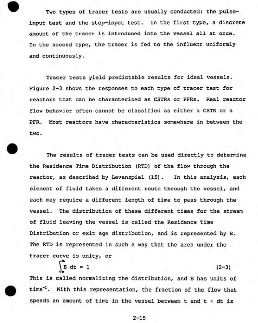
Two types of tracer tests are usually conducted: the
pulse-input test and the step-pulse-input test. In the first type, a discrete
amount of the tracer is introduced into the vessel all at once.
In the second type, the tracer is fed to the influent uniformly and continuously.
Tracer tests yield predictable results for ideal vessels. Figure 2-3 shows the responses to each type of tracer test for
reactors that can be characterized as CSTRs or PFRs. Real reactor
flow behavior often cannot be classified as either a CSTR or a PFR. Most reactors have characteristics somewhere in between the
two.
The results of tracer tests can be used directly to determine the Residence Time Distribution (RTD) of the flow through the
reactor, as described by Levenspiel (15). In this analysis, each
element of fluid takes a different route through the vessel, and each may require a different length of time to pass through thevessel. The distribution of these different times for the stream
of fluid leaving the vessel is called the Residence Time
Distribution or exit age distribution, and is represented by E.
The RTD is represented in such a way that the area under thetracer curve is unity, or
\ E dt = 1 (2-3)
This is called normalizing the distribution, and E has units of
time"^. With this representation, the fraction of the flow that
spends an amount of time in the vessel between t and t + dt is
PFR
response
CSTR response
Step Input Test Area = t
-^t
Area = i
1 - e-'/'
-*~t
Pulse Input Test
Area = 1-^ Width = 0~
E dt. (2-4) The fraction "younger" than ti is
E dt (2-5)
^}
ͣ'0while the fraction "older" than ti is
(e dt = 1 - [e dt (2-6)
These principles are shown in Figure 2-4.
The E curve is the distribution which describes nonideal flow
in vessels. It can be developed from a pulse-input tracer test by
dividing each measured effluent concentration, C^, by the total
area under the concentration-time curve, or
ICiAti
Ei = vvrt- (2-7)
For a step-input test, another type of curve, called an F
curve, can be developed. This is done by normalizing the
concentration vs. time graph for a step-input test by dividing
each measured effluent concentration, Ci, by Co, the tracer feed
concentration. In this way, the F values always range from 0 to
1. Figure 2-5 is an example of an F curve (15).
The E curve and F curve are related according to the
following equation:
dF
E = ^ (2-8)
HTD, or E curve
Fraction of exit stream
older than (i
Figure 2-4: Normalized Residence Time Distribution (RTD)
step input signal
Tracer output signal
or F curve
Figure 2-5: F curve from step-input tracer test. (15
(15)Hence, the slope of each segment of the F curve is a point on the
E curve. In this way, an E curve can be developed from a step-input test, and an F curve can be developed from a pulse-step-input
test.
Once the flow through a reactor vessel has been characterized by an E curve, predictions can be made about its behavior. Two
important parameters which can be used to characterize the RTD are the mean residence time, t, and the spread of the curve, which is
characterized by the variance, o" ^. For normalized distributions with discrete measurements, these parameters can be calculated
from the E curve as follows (15): •
t = ItiEiAt (2-9) cr^ = Iti^ EiAt - t} (2-10)
Several flow models have been developed to characterize
non-ideal flow behavior. These models describe the flow in terms of a
single parameter which would yield the same tracer response as for
the real reactor under consideration. Two such models that are
commonly used are the "tanks-in-series" model and the "plug flow reactor model with dispersion" (15). In the "tanks-in-series"
model, the reactor is assumed to behave as a series of CSTRs of
equal volume. Figure 2-6 is an example of the response to a
step-input tracer test (an F curve) for various numbers of tanks in
series, assuming the tracer is introduced into the first tank. As
ͣ
10
-0-9 0-8 L-07
-0-6
-/a
u- 0-5
-//f\
•0-4 0-3 0-2
"/
mi
sCI
-L
97 J
c10 20 30
t,f
Figure 2-6: Tracer response for tanks-in-series model, N is the number of equally-sized CSTR's in model. (16)
approaches that of a plug flow reactor (16). The number of CSTRs in series which would most closely approximate the behavior of the reactor can be determined from the mean and variance as follows
(15):
N = —S- (2-11)
c
where N is the number of equally-sized tanks.
For the tanks-in-series model, the F curve which would result
from a tracer test can be calculated as follows (16):
^ , --Nt. ,, Nt ,Nt,2 1 ,Nt,N_i 1 _ ,-,
F = l-exp(^^).{l+-^f (^1-)^ T^ . . . + {-:r) ,y,_.. , } (2-12)
t t t ^- t ^w i; .
where t is the mean residence time for the real reactor.
Similarly, the E curve which would results from the
tanks-in-series model is as follows (15):
E = -^ . (r)"'^ • t^\ . , exp(-t/t) (2-13)
Nt t (^ ^) •
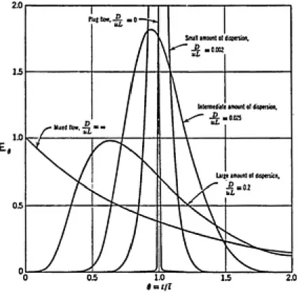
The "plug flow with dispersion" model assumes that the reactor acts like a PFR but has some mixing in the direction of flow. The parameter which measures the extent of axial dispersion is D/uL, the dispersion number. In this model, D is the parameter which characterizes the degree of backmixing during flow, L is
approximates a CSTR. Figure 2-7 shows the normalized tracer
response to a range of dispersion numbers (15). This plot has
been normalized such that
e = ^ and Ee = Et (2-14)
t
where t is the mean residence time.
Once the mean and variance are known, the dispersion number,
D/uL can be calculated using the following relationship (15):
^ = 2^ - 2(~)2(1 - e-""^-^) (2-15)
The Ee curve which would result from the plug flow with dispersion
model is as follows (15):
Ee = —r===^ exp(-.j^"^\. ) (2-16)
2Vjie(D/uL) 4e(D/uL)'
2.i Kinetics of Chlorine Decay and Pathogen Inactivation
Chlorine is a strong oxidant as well as a powerful
disinfectant. Natural waters usually have an oxidant demand due to inorganic and organic contaminants present. Chlorine added to drinking water will be consumed over time. It has been suggested
(17) in some cases that the dissipation of chlorine in natural waters can be approximated as a first order chemical reaction,
i.e.
C = Coe"'''' (2-17)
where C = chlorine concentration at time t
DISPERSION MODEL (DISPERSED PLUG FLOW)
2.0
Plug How, -^ = 0
Small amount of dispersion
\
uL§ =0.002Intermediate amount of dispersron
D = 0 025
Mixec How.
^
Liree amount of dispersicn
Figure 2-7: Plug flow with dispersion model, normalized
Co = chlorine concentration at time zero k = rate constant, time"'^
t = time
Each water supply is unique, containing different contaminants at different concentrations, and thus exhibits a different chlorine
demand. It is likely that the kinetics of chlorine dissipation can
not be simplified so easily, and that k varies over a wide range. However, a first-order assumption is a typical starting point in
attempting to characterize such kinetics.
The value used for C in the SWTR is the residual
concentration leaving the process unit in question. In the case of chlorine, this approach does not take into account the fact that chlorine is continuously dissipating throughout the vessel and that the concentration within the vessel is higher than in the effluent. If the oxidant demand of the water is high, a higher
dose of chlorine would have been added at the influent than was
detected leaving the vessel. The measured concentration in the effluent is an integrated measure of the residual chlorine for various elements of fluid spending different amounts of time in
the reactor. This means that some elements of the fluid were
exposed to a higher concentration of chlorine than others,
although perhaps for a shorter time, while other elements of fluid
were exposed to the effluent concentration. These variations in
chlorine concentration are not accounted for in the SWTR method
for calculating CT as a measure of disinfection effectiveness.
If the kinetics of chlorine dissipation are known and the RTD of the vessel can be characterized, this information can be used
to give a clearer picture of the actual extent of chlorine contact
and its corresponding degree of pathogen inactivation on the basis of exposure to the disinfectant. Using the E curve, each element of fluid can be assumed to be exposed to a different concentrationof chlorine for a different amount of time. The concentration to
which it is exposed depends on the residence time of that element of fluid. These incremental elements then can be summed up to give an "effective CT" which more accurately reflects the exposure conditions in the vessel. Mathematically, this can be expressed
as
effective CT = LEi • Ati • Coe""^^^ • ti (2-18)
In the preamble to the Surface Water Treatment Rule, EPA acknowledged that the method for computing the CT product is
conservative: "the product of C and T will reflect a substantially lower CT value than would actually be in effect and thus result in the determination of a substantially conservative estimate of
percent inactivation from the CT tables in the Rule." Applying Equation 2-18 for data generated from tracer studies at full-scale water treatment plants will lead to a more precise estimate of
pathogen inactivation and an indication of the degree to which the
Surface Water Treatment Rule over-estimates the degree ofͣ
•^.n EXPERIMENTAL METHODS
3.1 Description of Plants
Tracer tests were conducted at three water treatment plants:
the Patuxent Filtration Plant of the Washington Suburban Sanitary Commission (WSSC) in Laurel, Maryland; the Potomac Filtration Plant of the WSSC in Potomac, Maryland; and the Orange Water and
Sewer Authority (OWASA) Filtration Plant in Carrboro, North
Carolina. The WSSC system serves approximately 1.1 million people
in the area of Maryland immediately north of Washington, D.C. The
OWASA system serves approximately 60,000 people in the towns of Chapel Hill and Carrboro, North Carolina.
The Patuxent plant was studied because WSSC is considering adding ammonia at some location in the treatment train (after
chlorination) in order to reduce trihalomethane (THM) levels in
the finished water. Once ammonia is added, further formation of
THMs is halted. The Commission needs to make sure that enough
contact time with free chlorine is achieved to meet the CT
requirements of the Surface Water Treatment Rule before ammonia is
added. The addition of ammonia to chlorinated water creates combined chlorine or chloramines. Chloramines are much less
powerful disinfectants than free chlorine, and thus require much higher CT values.
The Potomac plant was studied to determine the contact time for free chlorine through the finished water reservoirs. Unlike
the Patuxent plant, WSSC has no immediate plans to explore the use
of ammonia for Potomac. However, there is some concern about the chlorine contact time available at the plant in its current
configuration. A relatively large amount of water passes through a relatively small set of finished water reservoirs, and WSSC is concerned that they might not be able to meet the CT requirement
of the Surface Water Treatment Rule at the Potomac plant.
Because of its proximity to the University of North Carolina at Chapel Hill, the OWASA plant was chosen for an additional set
of tracer tests for purposes of comparison with the WSSC plants.
Each of the three plants is described below.
3.1.1 WSSC Patuxent Filtration Plant
The Patuxent plant is part of the Washington Suburban
Sanitary Commission system, supplying about one quarter of the
water needed for the service area in east-central Maryland. The
source of supply is the Patuxent Reservoir, fed by the Patuxent
River. Average flow for the plant is 55 million gallons per day (MGD) and peak flow is 72 MGD. Water quality in the Patuxent Reservoir is good; the concentration of natural organic matter is fairly low (18) . The quality is relatively consistent, since the reservoir is able to absorb the shocks of higher contaminant
loadings that might wash down the river during the rainy season.
The Patuxent plant is a conventional treatment plant, according to the definition in the SWTR. Figure 3-1 is a
v&ter
polymer
cotgul&tion flocculttion fedlmentttlon
cblorine
illtrttion
ilwride
liiM (CtO)
to
distribtttion
fizdshed
Mter
storage
Figure 3-1; Flov Dlagrau, Patuxent Filtration Plant
the treatment train is conventional, the plant layout is not. Many of the process units are round and much of the flow is
radial, rather than linear. Figure 3-2 is a plan view of the
plant.
Raw water enters the rapid mix chambers in the main chemical
building where alum and polymer are added for coagulation. Raw water pH varies from 6.8 to 7.2, and is typically depressed to
between 6.2 to 6.5 by the addition of alum. Water temperature
varies from about 3°C in the winter to about 22°C in the summer.
The flow is then split into four different pipes, each of which
supplies one filter unit. Each filter unit has its own
flocculation and sedimentation areas. The sedimentation areas are
doughnut-shaped, surrounding the filters in each unit. Each unit
has six separate filters, arranged like pieces of a pie inside each sedimentation basin. These six filters are operated
independently, i.e., they are backwashed at different times and
have different run lengths. Each of the four filter units has two
chlorine injection points. Chlorine is injected into the pipes
through which the settled water travels on its way to the filters.
Chlorine doses average between 3.75 mg/1 and 4.25 mg/1, and residuals of about 2.0 mg/1 and 1.5 mg/1 are detected at the
effluents of the filters and clearwells, respectively.
Effluent from the six filters in each unit is collected into
rtv vtter
1 cbeiikical
building
filter 3
inter
exxluent blenders
to P&i
Figure 3-2: Scheiatic of Patuxent Filtration Plant
which are in-line mixers in the discharge pipes. Fluoride is
injected into these blenders, and the pH is raised to between 8
and 8.5 with lime (Ca(0H)2)- Finished water flows from the
effluent blenders to the seven reservoirs or clearwells. These
clearwells are operated in parallel, i.e., water can flow to any
or all of the reservoirs from the effluent blenders, depending on
the elevation of the water in each. The seven Patuxent tanks have
a combined storage capacity of 18.36 million gallons. Under
average flow conditions (55 MGD), the theoretical detention time
in the clearwells is 8 hours. On the opposite sides of the
clearwells, finished water is collected into the main distribution
lines. There are three lines leaving the plant for the
distribution system: Prince Georges 1 (PGl), Prince Georges 2
(PG2), and the pumping station. The PGl and PG2 lines are gravity
flow, and they are used for most of the year. The pumping station
is only used under very low flow conditions.
3.1.2 WSSC Potomac Filtration Plant
The Potomac plant is also part of the Washington Suburban
Sanitary Commission system. It supplies approximately three
fourths of the water used by the system. Average flow through the plant is 135 MGD, and peak capacity is 300 MGD. The source is the
Potomac River at the community of Potomac, Maryland. Water
quality is quite variable; raw water turbidities can range from
O.S^C in the winter to over 30°C in the summer. The Potomac plant is a conventional treatment plant according to the definition in the Surface Water Treatment Rule. Figure 3-3 is a schematic of the treatment operation, and Figure 3-4 is a plan view of the
plant.
The Potomac plant operates as two plants in parallel and, with a few minor exceptions, one side is the mirror image of the other. Raw water is pumped from the river to both of the two flocculation-sedimentation basins. Raw water pH varies between 7.0 and 8.8, averaging about 8.0. This pH is adjusted to between 8.2 and 8.6 with lime in the rapid mix chambers, which is the same point where ferric chloride and polymer are added for coagulation. Powdered activated carbon is added seasonally at this point to control tastes and odors. The water flows through the basins from south to north. The basins and finished water reservoirs on the east side are referred to as #2 and #4, while those on the west side are called #1 and #3, From the sedimentation basins, water flows directly into the banks of filters. There are 32 individual
filters; numbers 1 through 16 are on the west side and 17 through
32 are on the east side. Filtered water flows back south from the filters to the finished water reservoirs, located at the southernend of the plant.
After filtration, the water is fluoridated and chlorinated.
Both the fluoride and chlorine injection points are in the same
lines leaving the filters and flowing to the reservoirs. The
Mter
ivrric oblorid*
F^ (SMSontlly) lin« (CtO)
cotgulation ilocctCLttion s^diM&tttion Xiltrttion
chlorin* fluoride
to
diftribvtion
iiitisbed
wtter storage
filters 1 tbrough 16
fl00C\U4ti0R
sedimenbation basins #3 and #1
filters 17 through 32
flooov: ttion sedimexi bttiozi
bksias tZ Ukd *4
ty
pwps
to r%v distribution vater
Figure 3-4: Scheaatic of Potomac Filtration Plant
fluoride is added first, then the chlorine is applied at a point
480 feet downstream in the same pipe. During peak flow in the
east side, for example, these two injections are about 23 seconds
apart. The addition of chlorine and fluoride depresses the pH to
about 7.6. The average chlorine dose is 4.1 mg/1. Chlorinated
water then flows through the finished water reservoirs. These
tanks are rectangular, and they have a series of baffle walls that
were installed after the plant was completed. The finished water
reservoirs have a total capacity of 22 million gallons, so under
average flow conditions the theoretical detention time through
these tanks is 3.9 hours. When the plant is operating at peak
flow, this theoretical time decreases to 1.8 hours. An averagechlorine residual of 2.6 mg/1 is detected at the effluent of the
clearwells, and this residual varies between 1.6 mg/1 in the
winter and 3.3 mg/1 in the summer.
Water from both the east and west finished water reservoirs
flows to the finished water pumping station, located between the
two sets of tanks. From the station, water is pumped to the
distribution system.
3.1.3 OWASA Filtration Plant
The Orange Water and Sewer Authority plant serves the towns
of Chapel Hill and Carrboro, North Carolina. There are two
sources of supply for the OWASA plant: University Lake, which is
fed by Morgan Creek, and the Cane Creek reservoir. At the time
^^^
University Lake, mixing with the lake water, and being pumped to
the plant. (A new transmission line was under construction which would carry water directly from the Cane Creek reservoir to the plant, bypassing the lake.) Plant capacity is 8 MGD, and it is usually operated at or near this flow rate. The demand varies greatly with the seasons, primarily because of the presence of the
University of North Carolina in Chapel Hill. During the school
year, the plant experiences a much greater demand than in the
summer due to the transient student population. A schematic of
the OWASA plant is shown in Figure 3-5, and Figure 3-6 is a plan
view of the facility.
Raw water is pumped to the plant from University Lake.
Temperatures in the plant vary from 5°C in the winter to over 40°C in the summer. The pH of the raw water varies between 6.9 and
7.1. In the rapid mix area, alum and polymer are added as
coagulants. Powdered activated carbon and potassium permanganate
are sometimes added at this point to control tastes and odors, and
iron and manganese, respectively. Addition of alum depresses the
pH to between 6.2 and 6.5. From the rapid mix basins, water flows through the flocculation chambers, then into a header which feeds
all five of the sedimentation basins. Each sedimentation basin
normally supplies one filter, although flow can be diverted to any of the five filters from any of the sedimentation basins.
Chlorine is added at five locations, the five influents to the filters. The chlorine dose varies between 4 mg/1 and 7 mg/1, with an average of about 5 mg/1. Chlorine residuals of approximately
polpwr
P&C (sMSOMlly)
Bfn04 if^MomHj)
coftgnlation sediaenUtion
olilorint floorid* ItOH corrosion iBtdUtor
liltrttion
to
distribution
vkttr
r«pid nix
b&sins
iloc
bftsins Md b4sizi i
s*d
bftsin 2
Md b*fin 3
Md
buin 4
s«d b4sin 5
to
diftribution
filter 1 iilt«r 2 filter 3 filter 4 iilUr 5
Qr
-:?
clearvell
Figure 3-6: Schematic of 0¥ASA Filtration Plant
2.5 mg/1 and 1.9 mg/1 are typically detected at the effluent of
the filters and clearwell, respectively. The chlorine demand of
the water is appreciably higher that that of the WSSC systems.
After filtration, water from all five filters is collected in
a common pipe, and flows into the clearwell. Fluoride is added in
this line, upstream of the clearwell, and the pH is adjusted to
about 7.3 with caustic soda (NaOH). The clearwell is rectangular
and is not baffled. It has a capacity of 1.5 million gallons, and
the theoretical detention time under average flow is 4.5 hours.
The inlet and outlet structures are located on the same side ofthe tank. Finished water is pumped from the clearwell to the
distribution system.
3.2 Experimental and Analytical Methods
Two types of tracer tests were conducted at the three water
treatment plants: step-inputs and pulse-inputs. Fluoride was used
as the tracer in most of the tests because it is non-reactive and
non-toxic, and it is already used at the three plants, making it
readily available and convenient. Sodium was used for two pulse
input tests in order to verify the fluoride results. Generally,
step-inputs were done to analyze the residence time distributions
(RTDs) of finished water reservoirs and pulse-inputs were done to
determine the RTDs of filters. This is because all three plants
add fluoride after filtration and before finished water storage,
and the equipment for the step-input tests was already in place.
3.2.1 Step-Input Tests (Finished Water Reservoirs)
In a step-input test, the tracer is fed to the reactor vessel
continuously, and its concentration in the effluent is monitored
over time. (See Section 2.5 for theory.) Under normal operating
conditions at all three plants, fluoride is fed continuously into
the water upstream of the clearwells.
For the step-input tracer tests, the fluoride feed to the
clearwells was turned off initially. This was considered the
start of the test, "time zero." The fluoride concentration in the
effluent of the tanks was monitored over time until the
concentration of fluoride leaving the tanks decreased to the same
concentration as the raw water. If another test was to be run atthis point, the fluoride feed to the clearwells was turned back
on, and the concentration in the effluent was monitored. Thistime, monitoring continued until the fluoride concentration in the
effluent increased to the level of the feed concentration. In
this way, the second test could be used to verify the results of
the first.
As a rule of thumb, the duration of the step-input test was
at least three times the theoretical detention time (volumedivided by flow rate) through the basins (19). The time between
sample collection usually was some fraction of the theoretical
time, ranging from 1/4 to 1/8. After about two theoretical
detention times, the sampling frequency was decreased. The flow
rate through the clearwells and the volume of water in the clearwells was kept constant throughout each test.
Step-input tests were done for the finished water reservoirs at both the Patuxent and Potomac filtration plants. At Patuxent, fluoride normally is added at the effluent blenders. All of the filtered water treated at the plant passes through these blenders before reaching the clearwells. Step-input tests were done over a two-day period. May 17 and 18, 1989. Under normal operating
conditions, the theoretical detention time through the reservoirs is 8 hours (18.36 million gallons of storage divided by 55 million gallons per day), so it was determined that only one step-input test per day could be conducted.
On the first day, May 17, the fluoride feed to the clearwells was turned off, and on the second day, May 18, it was turned back on. The typical fluoride feed concentration is 1.0 mg/1. Because there are two lines leaving the plant for the distribution system, two tracer curves were developed each day. Both of the lines, PGl and PG2, can carry water from any or all of the seven reservoirs. Samples were collected directly from the lines, not from the sampling taps in the laboratory.
The Guidance Manual (10) recommends that tracer tests be
that could be sustained for the duration of the test. The maximum
flow yields the critical, or shortest, contact time. If the plant
can meet the CT requirement at this flow, then it can meet it at
all other flows. A detailed protocol was developed as a part of
this project so that plant personnel could repeat the tracer test
at other flow rates. Appendix II contains this protocol.
The other critical condition for meeting the contact time
requirement is the volume of water in the clearwells. The lowest
level of water in the reservoirs yields the shortest contact time.
Therefore, the clearwells at Patuxent were drawn down to half of
their maximum capacity for the tracer tests. This is as low as
they are ever operated. Samples were collected at intervalsranging from a half hour to four hours, and the sampling duration was 24 hours.
At the Potomac plant, fluoride is injected into the main
lines leaving the filters and flowing to the clearwells. Since
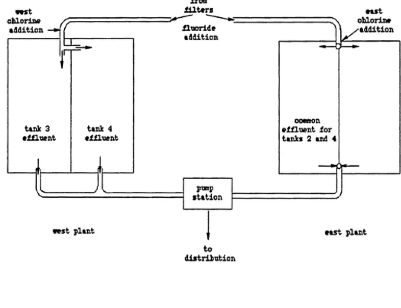
the plant operates as two plants in parallel, the tracer testswere conducted through only one half of the plant. The east side
of the plant was isolated from the west side for the duration of the tests. The east side was chosen because the influent and
effluent structures are common to both tanks, unlike the west side
which has two separate influent and effluent lines (see Figure
3-7).
oblorine addition
t&xtk 3
•filnent
tank 4 tfiluent
iroffi lilt«rs Hooride
Addition
MkSt
oblorin* addition
COMMOn
effluent for tanks 2 and 4
pwip station
vest plant
t
to distribution
east plant
Figure 3-7: Diagram of Influent and Effluent Structures,
Four tracer tests were conducted over a two-day period,
August 22 and 23, 1989. Two flow conditions and two reservoir
levels were studied: 150 MGD and 75 MGD, and full and half-full reservoirs. These cover the range of conditions normally
encountered at the plant. The first day's tests used 150 MGD and
75 MGD, both with the reservoirs full. On the second day, the reservoirs were lowered to half-full, and the same flow rates, 150 MGD and 75 MGD, were used. Theoretical detention times for theseconditions varied from less than one hour to three and one half
hours. Lengths of the tests ranged from three hours to ten hours, and sampling frequency was as short as five minutes in one test and as long as one hour in another. Samples were collected with a
dipper on a string which was lowered into the effluent mixing
chamber for tanks 2 and 4.
3.2.2 Pulse-Input Tests (Filters)
In a pulse-input test, a discrete amount of concentrated tracer is added all at once to the reactor influent, and its
concentration in the effluent is monitored over time. (See
Section 2.5 for theory.) For most of this project, the tracer
used was concentrated hydrofluosilicic acid, H2SiF6. This compound
is a byproduct of the fertilizer industry, and is commonly used by
water treatment plants as a source of fluoride because it is