degree. April, 2000, 61 pages. Advisor: Robert M. Losee.
The effects of dimensionality reduction on information retrieval system performance are studied using Latent Semantic Indexing (LSI) on simulated data. The authors hypothesize that LSI improves retrieval by improving the fit between a linear language model and non-linear data such as natural language text. The study analyzes how the values of three variables bear on optimizing k, the system’s representational dimensionality. The variables studied are: the correlation between terms, the dimensionality of the untransformed termspace, and the number of documents in the collection. Using multinormally-distributed, stochastic matrices as input, precision/recall and average search length (ASL) are computed for differently modeled retrieval situations. Results indicate that optimizing k relates to the type and degree of correlation found in the original termspace. Findings also suggest that a more nuanced simulation model will permit more robust analysis.
Headings:
Information Retrieval
Information Retrieval—algorithms—Latent Semantic Indexing Natural Language Processing
THE DYNAMICS OF DIMENSIONALITY REDUCTION FOR INFORMATION RETRIEVAL:
A STUDY OF LATENT SEMANTIC INDEXING USING SIMULATED DATA
by Miles J. Efron
A Master’s paper submitted to the faculty of the School of Information and Library Science of the University of North Carolina at Chapel Hill
in partial fulfillment of the requirements for the degree of Master of Science in
Information Science
Chapel Hill, North Carolina April, 2000
Approved by:
___________________________
1. Introduction
Latent Semantic Analysis (LSA) provides a robust method for automated discovery and representation of high-level semantic features of natural language text (Landauer, Foltz, and Laham, 1998; Landauer and Dumais, 1997). In its application to Information Retrieval, LSA is employed during indexing to improve the mapping between queries and documents. By using the singular value decomposition (SVD) (Forsythe, Malcolm, and Moler, 1977), a linear algebraic dimensionality reduction method, Latent Semantic Indexing (LSI) represents terms and documents in a high-dimensional vector space whose axes derive from patterns of term/document co-occurrence in the original data (Deerwester et al., 1990). LSI's proponents argue that this compressed representation of the original data brings the collection's “latent semantic structure” to the fore, thus improving both recall and precision.
clear that a range of dimensions somewhere between 50 and 300 will optimize
performance; other applications may require more dimensions1. However, why this is so remains open to question.
Experimental studies have attacked the question pragmatically: “In our tests, we have been guided by the operational criterion of 'what works best'” (Deerwester et al., 1990, p. 402). This approach yields clear results. However, experimental studies have lacked a developed effort to explain the effect of dimensionality reduction. On the other hand, more analytical approaches (Ding, 1999; Story, 1997) offer powerful models of LSI. This work lends LSI a much-needed theoretical basis, but fails to situate
dimensionality reduction in the larger context of an IR system. What is missing from both approaches is an understanding of the relationship between the SVD and the language model assumed by actual IR systems.
The current study speaks to these omissions. Empirical factors such as the correlational characteristics of the original termspace, the number of documents in the collection, and the number of terms used to construct document vectors bear on an LSI system's optimal dimensionality. This study analyzes these factors, with an eye towards explaining the dynamics of LSI dimensionality reduction. Besides asking which
and average search length (ASL), all of which are described below. For the purposes of this study, we define optimal dimensionality (kopt) to be the range of values that will generate the best ranking of documents when used to truncate the LSI space.
By tracking retrieval performance across diversely modeled LSI implementations, we analyze the interaction between system variables and LSI dimensionality reduction. We model LSI retrieval by using stochastic, multinormally-distributed binary matrices as input to the system. In favor of actual term-document matrices, we test retrieval using probabilistically simulated data. This method allows us to accentuate the relationship between optimal dimensionality and "empirical" data characteristics. Put differently, it allows us to analyze dimensionality reduction while controlling the fit between our language model and the data themselves. By simulating LSI with an explicitly articulated language model we gain control over the variables that influence the value of
dimensionality reduction.
Section 2 provides an overview of LSI and the SVD. Section 3 describes previous efforts to optimize dimensionality reduction for IR. In section 4 we outline the simulations, describing the variables that they allowed us to control. The 5th section considers the problem of LSI dimensionality optimization as it emerged in the
2. Latent Semantic Indexing and the Singular Value Decomposition
Overview of LSI
Information retrieval systems attempt to present users with documents that are relevant to a stated information need (Salton, 1989; van Rijsbergen, 1979). Although the details of this process vary widely across systems, traditional IR implementations judge the similarity between queries and documents by comparing the terms that appear in each. After years of refinement and tuning, the term-matching approach to IR yields solid, well-understood performance. However, the question remains: how well does the term-matching approach capture actual features of meaning in text? Has the user chosen to express his query in the best possible terms? Do the system's indexing terms capture the “aboutness” of the relevant documents in the collection? Furnas et al. (1987) suggest that systems based on term matching suffer from their overtly literal representation of
intellectual content.
Latent semantic indexing attempts to overcome this literalness. Deerwester et al. (1990) argue that LSI improves upon traditional retrieval by obviating two major
limitations of term-matching: synonymy and polysemy. Synonymy hurts an IR system's recall. If a user requests information about cars, a strict term-matching system will fail to identify documents about automobiles as relevant. On the other hand, polysemy causes precision to suffer. In a term-matching system a query on the West Bank may return documents about The Bank of the West, a match in the term-space, but not in most users' semantic space. In these cases the terms used to represent abstractions such as the users' information need and the aboutness of each document fail to operate as useful
LSI addresses the shortcomings of term matching by viewing the gap between a document's (or a query's) articulation and its meaning as a noisy data problem.
Deerwester et al. (1990) describe LSI in terms of statistical noise reduction:
The proposed approach tries to overcome the deficiencies of term-matching retrieval by treating the unreliability of observed term-document association data as a statistical problem. We assume there is some underlying latent semantic structure in the data that is partially obscured by the randomness of word choice with respect to retrieval. We use statistical techniques to estimate this latent structure, and get rid of the obscuring “noise.” (Deerwester et al., 1990, p. 391)
The goal of LSI is to find a representation of a document collection that manifests its “latent semantic structure.” Polysemy and synonymy obscure this structure much as observational error or rounding errors obscure the relationships between variables in standard data analysis. Assuming that the collection possesses a useful semantic structure, LSI attempts to remove the noise introduced by these errors, resulting in an improved representation.
To improve the representation of a collection LSI employs a linear algebraic dimensionality reduction method called the singular value decomposition. Explaining LSI procedurally, Christopher Manning and Hinrich Scheutze write:
in the process of [LSI] dimensionality reduction, co-occurring terms are mapped onto the same dimensions of the reduced space, thus increasing similarity in the representation of semantically similar documents. (Manning and Scheutze, 1999, p. 559)
approximates the dataset. By analyzing a corpus LSI might learn, for instance, that car and automobile tend to appear in similar contexts. In light of this pattern of
co-occurrence, the final LSI representation may conflate car and truck into a single factor that maps roughly to road-vehicles (in a real LSI system, the high number of derived factors prohibits this sort of reification). In this way, information that warranted two dimensions in the original space is now projected onto one, more expressive dimension. Dimensionality reduction improves IR data representation because lexical terms are rarely orthogonal. The distance between terms is rarely sufficient to permit them to act as ideal markers of a high-level concept. This problem is especially acute given an IR language model that assumes term independence. The vector space IR model (VSM), upon which LSI is based, assumes that the distribution of each term across documents is statistically independent of the distribution of all other terms. For a linearly based language model such as the VSM’s, the presence of a term t in a document d has no bearing on the likelihood of term w’s presence in document d. In the case of natural language terms, the assumption of independence is patently wrong. It is our contention that LSI improves the linear similarity model by assuaging the impact of this error. That is, given a non-orthogonal termspace and a system with no ability to model the
relationship between terms, LSI improves the fit between the language model and the data by recasting the data into an orthogonal semantic space whose axes are informed by term-document patterns of correlation.
By analyzing the columns of Table 1 it is clear that some documents are about cars while others are about marathons. One document (d4) seems to be about both. By analyzing the rows it becomes tempting to generalize and say that documents in this corpus are about two topics, driving and running; the terms cars and marathons approximate these higher-level concepts. However, the behavior of d4 makes this generalization difficult.
d1 d2 d3 d4 cars
marathons
1 1 0 1 0 0 1 1 Table 1. A tiny corpus of documents.
d1 d2 d3 d4 driving
running
1 1 0 0 0 0 1 1 Table 2. A tiny corpus of documents.
How discrete are the categories, driving and running, as evidenced by our corpus? In the ideal case, term vectors are orthogonal to each other. Mathematically this means that their dot product equals zero. Semantically it implies that they mark discrete patterns of usage. In other words, the closer two term vectors are to orthogonality, the more information they contain, and therefore, the more help they will be in classifying the documents that form them.
In our example the presence of d4 frustrates our hope for orthogonal terms. The terms in the tiny database are not orthogonal (their dot product equals 1, not 0). As a counter example, consider the database in Table 2. Here we have replaced cars and marathons with different terms to represent our documents, driving and running. This
example the representational axes driving and running are orthogonal. They permit an unambiguous classification of the documents.
In practice lexical terms are rarely orthogonal. Synonymy, polysemy, and simple lexical imprecision argue against maximally expressive natural language terms. LSI operates by creating artificial representational factors which are orthogonal. Because these artificial factors are more expressive than the original term vectors (insofar as they capture the greatest variance while avoiding covariance), an LSI retrieval system can model the original covariance among data in a space of reduced dimensionality. In other words, LSI works on the assumption that the original n-dimensional representation (for example by terms) is noisy; we assume that many of the n dimensions are redundant, or non-orthogonal. Thus LSI creates artificial, orthogonal dimensions with which to replace the original axes. Of these, system designers choose to represent their data with the k† n strongest of these factors. By choosing an appropriate k value, we manage to represent the original covariance among documents while omitting the noise that resides in the n-dimensional space.
axes, the LSI system capitalizes on the strongest patterns of association in the database while dropping the redundant, weak patterns from its representation.
Singular Value Decomposition: The Implementation of LSI Dimensionality Reduction
To make these artificial, orthogonal factors, LSI employs a linear algebraic process called the singular value decomposition (SVD). While a complete description of the SVD is beyond the scope of this paper, we offer a working overview of the process. Forsythe, Malcolm, and Moler (1977) and Strang (1993) give thorough treatments of the
mathematics of SVD. Berry and Dumais (1995), and Deerwester et al. (1990) offer good discussions of the suitability of SVD for LSA. Manning and Scheutze (1999) describe the SVD in the larger context of natural language processing. Our discussion is drawn from all of these treatments.
The singular value decomposition is a factor analytic approach to dimensionality reduction. It is similar to principal components analysis (Oakes, 1998) and
multidimensional scaling (Bartell, Cottrell, and Belew, 1992) insofar as it involves the creation of orthogonal factors based on observations of putatively non-orthogonal variables. Unlike other factor analytic dimensionality reduction techniques, SVD offers three important qualities:
1. ability to operate on non-square matrices
2. ability to represent both rows and columns (i.e. terms and documents) of a matrix in terms of derived factors
These qualities allow the SVD to operate on the term-document matrices common to vector-based IR models. Moreover, the explicit representation of terms allows an LSI system to represent queries in the reduced semantic space without re-computing the SVD. Finally, and most crucial intellectually, the selection of the k largest factors will result in the best rank-k approximation of the original data, in the least-squares sense.
To compute the singular value decomposition, we begin with a matrix A. In the case of LSI, this matrix will usually be composed of term vectors on the rows and
document vectors on the columns. A cell aij shows the number of times term i appears in document j. In actual practice, these cells would undergo local and global
transformations to create the final matrix. For the sake of simplicity, however, we model the simplest case: a binary representation of term-document associations. Thus each cell aij shows a 1 if term i appears in document j or a 0 otherwise.
In the singular value decomposition, the m‰n rectangular matrix A with rank=r is factored into the product of three special matrices:
A = TΣΣD' (1)
Matrix T represents the rows of the original matrix A. D' represents the columns. In the case of information retrieval, T shows each term as a column, with the artificially derived factors as rows. D' shows documents on the columns, represented by vectors of factors. The important point is that both terms and documents are now represented in the same space, along the orthogonal axes derived by SVD.
Like principal components analysis and other factor analytic techniques, SVD derives its representational factors by observing patterns of co-occurrence between rows and columns in the original matrix. Each factor derived by SVD describes as much covariance among the data as possible while accumulating the least possible covariance with other factors (i.e. remaining orthogonal). Thus the first factors derived by the decomposition reflect the strongest variations in the original matrix. Because SVD by definition will find r factors for a matrix A where rank(A)=r, as we approach the rth factor, the amount of variance described by each axis will be very small. The strength of a factor i is represented by the ith singular value (óii). By convention, the singular values appear in the diagonal matrix Ó in decreasing order or magnitude.
The dimensionality reduction in LSI comes about by truncating the matrix Ó and then recombining it with the matrices T and D'. By choosing a dimensionality k and setting all singular values i for i>k equal to 0, by matrix multiplication, we reduce T and D' to k dimensions. This amounts to having projected our original matrix A onto the best k-dimensional space, in the least-squares sense. The benefits of LSI arise in the
the truncation phase of LSI allows us to represent our data along maximally expressive axes (axes 1-k), while rejecting the ostensibly noisy axes k-r from our representation.
3. Optimizing the Representational Dimensionality
Much of the putative advantage of LSI over the standard vector space model lie in the truncation of the system's representational space. Given a t‰d input matrix the traditional vector space model represents documents in Ât space. LSI, on the other hand, represents
the same documents in Âk space, where k† t. Because a matrix's last singular values
tend to be very small (and consequently low in significance), we assume that omitting the factors associated with those values removes random, redundant variance from our representation. Deerwester et al. (1990) liken the dimensionality truncation to noise reduction:
Ideally we want enough dimensions to capture all the real structure in the term-document matrix, but not too many, or we may start modeling noise or irrelevant detail in the data. (Deerwester et al., 1990)
Other research suggests that by finding an optimal k, we may learn useful characteristics of our dataset. For instance Yang (1995) argues that weak singular values may be used to find and remove unimportant words from the term-document matrix. Jiang and Littman (forthcoming) propose a method for cross language retrieval (Approximate Dimension Equalization) that optimizes the matrix A as A' by representing documents along the first k SVD-derived dimensions. ADE then normalizes all dimensions above k by ók.
be tossed away,” writes Roger Story, “is something of an art” (Story, 1996, p. 332). Ideally we would choose a dimensionality k where the associated LSI factors cease to express useful variance across terms and documents and start to model random and redundant variation. Such a k-dimensional space would collocate like documents and separate dissimilar ones, assuming a Euclidean similarity model such as the cosine or dot product.
Approaches to determining optimal k have fallen chiefly into two camps: experimental and analytical approaches. Most experimental treatments of LSI at least mention the issue of dimensionality selection. Analytical studies, on the other hand, tend to treat the problem of dimensionality reduction in the larger context of supplying a theoretical foundation for LSI. In the remainder of this section we outline the findings of several studies with an eye towards what has been solved and what remains unknown regarding optimal k.
The classic study of LSI, Deerwester et al. (1990), confronts optimal dimensionality from an engineering perspective:
We believe that the representation of a conceptual space for any large document collection will require more than a handful of underlying independent "concepts," and thus that the number of orthogonal factors that will be needed is likely to be fairly large....Thus we have reason to avoid both very low and extremely high numbers of dimensions. In between we are guided only by what appears to work best. (Deerwester et al. 1990, p. 396)
For tests run on the MED dataset, Deerwester et al. find that mean precision doubles by moving from a 10-dimensional representation to a 100-dimensional space (p. 402). Beyond 100 dimensions, they find little performance gain.
context of language acquisition), their method and findings are analogous to Deerwester's et al. Arguing that “the correct choice of dimensionality is important to success,”
Landauer and Dumais test their system's ability to answer vocabulary questions after projecting a training corpus onto spaces of differing dimensionality. They find that optimal performance occurs for k > 300:
choosing the optimal dimensionality of the reconstructed representation approximately tripled the number of words the model learned as compared to using the dimensionality of the raw data....[It] is clear that there is a strong nonmonotonic relation between number of LSA dimensions and accuracy of simulation, with several hundred dimensions needed for maximum performance, but still a small fraction of the dimensionality of the raw data. (Landauer and Dumais, 1997, p. 220).
Landauer and Dumais argue that the reduction of a t-dimensional problem to a k† t-dimensional problem improves similarity judgments by representing data along axes that capture the original data's meaningful variations.
Experimental approaches such as these are useful insofar as they offer results that are easy to interpret: a suggestion that kopt will probably lie somewhere between 100 and 300. However a spread of 200 dimensions leaves a lot of room for system tuning. More problematic is the difficulty of understanding why one system should be optimized at 100 dimensions while another performs best at 300. Landauer and Dumais write:
How much improvement results from optimal dimensionality choice depends on empirical issues, the distribution of interword distances, the frequency and composition of their contexts in natural discourse, the detailed structure of distances among words. (Landauer and Dumais, 1997, p. 215)
Roger E. Story (1996) addresses the suitability of LSI from a strictly analytical perspective:
We specifically do not look at the empirical evidence for the effectiveness of LSI--this already has been done by others--but limit ourselves to expanding the set of theoretical models from which the LSI algorithm can be derived. (Story, 1996, p. 329)
Likening LSI to a Bayesian regression model, Story argues that the practice of truncating Ó is suitable in two regards. First it permits us to remove “apparently erroneous”
information from our data. In the context of Story's regression analogy, the information contained in small singular values contradicts our Bayesian prior knowledge about the data (p. 339). Secondly, Story rephrases the common assertion that small singular values express statistically insignificant variance. Using the vocabulary of orthogonality, Story reasons that if the input matrix A were orthogonal, the matrix Ó would show some constant c on the main diagonal with 0 elsewhere. In this case the ratio of ó1 to ór would be 1 for c ¹ 0. By truncating Ó we bring the ratio of the largest to smallest singular values closer to 1. Thus if we were to reconstruct the original matrix as A'=Tk ÓkDk, that
reconstruction would be closer to orthogonality than the original matrix A: increasing the number of nonzero singular values kept in LSI eventually leads to diminishing returns even when there is no error or noise in the data (X): at some point the errors...due to increasing nonorthogonality become greater than the value of the additional information retained.... (Story, 1996, p. 339)
According to Story, the smallest singular values are not useful because they make the axes of our data representation less informative.
such a process is the first left singular vector. Likewise, the best two-dimensional parameterization of the distribution uses the first two left singular vectors. By adding more dimensions to the probability function, Ding proves that the likelihood of the function grows. Why doesn't a representation at full rank provide the best results, then? Ding argues:
the statistical significance of each LSI vector is proportional to the square of its singular values [sic] (ói2 in the likelihood).
Therefore, contributions of LSI vectors with small singular values is much smaller than ói itself as it appear [sic] in the SVD....
We further conjecture that the latent index vectors with small eigenvalues contain statistically insignificant information, and their inclusion in the probability density will not increase the likelihood. In LSI, they
represent redundant and noisy semantic information. (Ding, 1999 p. 62). By adding dimensions to a representation, one eventually reaches a point where adding another singular vector will not improve the likelihood estimate for the parameters of the underlying process. Like the experimentalists, Ding argues that each matrix will possess “an optimal semantic subspace with much smaller dimensions [than the original
dimensionality] that effectively capture the essential semantic relationship between terms and documents...” (Ding, 1999 p. 64).
to be addressed in the literature is the dynamics of discovering optimal k. According to Ding, the relationship between optimizing k and the original data matrix requires “further clarification” (Ding, 1999 p. 64). The remainder of this paper describes our attempt to offer such clarification.
4. Simulating LSI
Despite important research the problem of optimizing LSI dimensionality remains an open issue. Experimental studies such as Landauer and Dumais (1997) and Deerwester et al. (1990) have yielded concrete heuristics: for a realistic dataset optimal k will probably
lie in the range of 50-300. Analytic studies, on the other hand, have justified the practice of singular value truncation mathematically. The work of Story (1996), Ding (1999), and Hoffmann (1999) situates LSI in the well-theorized context of Bayesian regression, MLE analysis, and probability theory, respectively. Bartell et al. (1992) show that LSI
constitutes a special case of multidimensional scaling. Analytical work such as this proves that LSI works. It may even describe why LSI works.
What remains open to investigation, though, is how LSI works. That is, given a particular dataset in a particular retrieval environment, what makes one dimensionality better than another? What happens to the arrangement of documents in a system's semantic space as we change its dimensionality? What are the empirical characteristics of data that bear on optimizing k? These questions are difficult to answer using
traditional research methods. Experimental studies fail to address them primarily because they lack control over independent variables against which to test the effects of
However, the price of this fine perspective is the concomitant difficulty in accounting for complex multivariate interactions.
We approach the problem of LSI dimensionality reduction by simulating a retrieval task with stochastically generated data. Using Mathematica, a mathematical computing environment (Wolfram, 1999), we create random term-document matrices that conform to certain criteria (discussed below). We then perform standard LSI retrieval on the artificial dataset, tracking the success of the system as k varies. Using artificial data permits explicit control over the system. Moreover, results from the simulations are easy to interpret. This is for two reasons. First, the data are generated using a
well-understood, highly simplified stochastic model. By omitting much of the complexity of real linguistic data, the relationships between independent and dependent variables come to the fore. Second, simulating retrieval allows us to express system performance in terms of familiar IR performance metrics.
The Task
subjected to local and global weighting. However, for the sake of clarity we omit this step.
Having created a term-document matrix A, the query is represented as a pseudo-document: an n-dimensional vector with 1 on each dimension that corresponds to a user-specified term, and 0 elsewhere.
The task of the system is to rank all documents in order of their similarity to the query. Similarity between a query q and a document d is thus calculated by taking the inner product of the two vectors:
Sim[d, q] = d . qT . (2)
Retrieval involves comparing the query to each document in the database, ranking documents in order of their similarity to the query (Formula 2).
In the case of LSI, however, the m‰ n-dimensional term-document matrix A is subjected to the singular value decomposition before retrieval. Using Formula 1, we obtain three matrices T, Ó, and D'. T represents terms in the semantic space of A. D' represents documents in the same space. Matrix Ó contains the singular values for A. We represent the query and the and documents using the k strongest LSI-derived factors. This involves projecting both terms and documents onto k space. For this procedure we follow Manning and Scheutze (1999). We restrict our representation to k dimensions by taking only the first k rows from T, Ó, and D' to create: Tt‰k, Ók‰k, and Dd‰kT. Documents are represented by the matrix B = Ók‰k . Dd‰kT. Following Berry and Dumais (1994) the query vector q is represented by formula 3,
These transformations produce the best k-dimensional representations of documents and the query, in the least-squares sense. Using Formula 4, we calculate the similarity between a query and document in k space as:
Sim[q', d'] = q' . d' (4)
For each dimensionality k, we rank all documents against q in k-space, calculating the following performance measures at k: precision at 100% recall, precision at 75% recall, precision at 50% recall, precision at 25% recall, and the average search length (ASL)2.
The Data Model: The Multivariate Normal Distribution
To afford maximal control over the experiments, we perform LSI on artificial,
probabilistically modeled term-document matrices. Constructing an artificial m‰n term-document matrix proceeds by making m n-dimensional term-document vectors. To do this we assume that document vectors do not occur randomly. Instead we assume that they are generated by some underlying stochastic process. For these experiments we model this process using the multivariate normal (also called the multinormal) distribution function, whose probability density function is given in Formula 53.
( ) ( )/2
2 / 1 1 ) 2 ( 1 )
( µ µ
π − Σ − − − Σ
= x x
p e
f x (5)
where ì is the distribution's mean vector, and Ó is its covariance matrix. Informally, this implies that individual terms are normally distributed across documents, and that
combinations of term occurrence in documents are also normally distributed. While assuming normal distribution of terms across documents is dubious, it is useful for
designed to work on normally distributed data. This is the case because the normal distribution assigns the highest probability to events closest to the mean. “So the least-squares solution is the maximum likelihood solution” if the data are normally distributed (Manning and Scheutze, 1999, p. 565). By modeling data with the multinormal
distribution, then, we optimize the fit between the data and LSI. How this impacts the relation of our artificial matrices to real data remains to be studied.
Multinormal Parameters
The multivariate normal distribution takes two parameters, the mean vector, ì, and a covariance matrix, Ó. In the context of IR, ì is an m-dimensional document vector, where m is the number of terms in the collection. ìi specifies the mean frequency of
termi in a document. Ó is an m‰m ij is the
covariance between terms i and j. Thus Ó is symmetrical, with the variance for each term on the main diagonal.
For our simulations we assume that two stochastic processes are at work: one that creates relevant documents and one that creates non-relevant documents. Thus we create a separate distribution for each set of documents. Because each distribution creates documents in the same term-space, each distribution uses the same covariance matrix Ó. However, we assume that relevant and non-relevant documents will have different mean vectors. That is, relevant documents are more likely to score high on terms that are specified in the query than are non-relevant documents. Table 3 gives a simplified example in a 2-dimensional term-space:
Vector Values query: {1, 0} ìrel: {1, 0} ìnon-rel: {0, 0}
Table 3. Simple relationship between a query and mean vectors for relevant and non-relevant documents.
We assume that the query offers the best prediction of a relevant document. Thus in the simplest case we use the query itself for ìrel. Because the term-document matrix will generally be sparse, in the simplest case we set ìnon-rel equal to an m-dimensional vector of zeroes.
In actual practice, the simplified mean vector representation shown in Table 3 yields unrealistically high discrimination between relevant and non-relevant documents. Figure 1 illustrates this problem.
Figure 1. Probability functions for relevant and non-relevant documents modeled by parameters shown in Table 34
To mitigate this problem we choose non-binary values with which to populate mean vectors: a mean for query terms in relevant documents, and a mean for all other terms. For our simulations, we chose .25 and .025 for these values, respectively. The vectors shown in Table 3 thus become the values shown in Table 4:
Vector Values query: {1, 0} ìrel: {.25, .025}
ìnon-rel: {.025, .025}
Table 4. The relationship between a query and mean vectors for relevant and non-relevant documents as implemented in the simulations.
Figures 2a and 2b show the populations modeled by these parameters.
Figure 2a. Relevant documents
Figure 2b. Non-relevant documents
After modifying the term frequencies in our mean vectors, the patterns of term
Concomitantly, retrieval of relevant documents becomes more challenging, allowing changes in system parameters to affect observable results.
The covariance matrix Ó describes how widely each term's frequency varies from the mean and how each term covaries with each other term. A simple covariance matrix for a 2-term dataset is illustrated in Table 5.
Term1 Term2
Term1 .5 0
Term2 0 .5
Table 5. A simple covariance matrix
Here both terms exhibit the same dispersal from the mean: .5. Likewise, they do not covary at all. The simplest covariance matrix is thus a diagonal matrix with of some constant variance score. By increasing the covariance between terms, stronger inter-term relationships may be modeled. We predict that higher covariance between terms moves the distribution away from orthogonality.
Our simulations model 3 types of term variance. In the simplest case (term independence), we use a covariance matrix of the type shown in Table 4: a matrix of zeros with a constant on the main diagonal. To complicate the model a bit, our baseline settings add a representation of pairwise covariance to Ó. This configuration appears in Table 6:
Term1 Term2 Term3
Term1 .5 .05 0
Term2 .05 .5 .05
Term3 0 .05 .5
The third type of covariance (distant covariance) adds to the baseline variety. Here we distribute all variance for termi not accounted for by termi-1 and term I+1 across all other terms. If variance for termi =.05 and pairwise covariance=.05, this model sets the covariance between termi and all other terms =.5 ‰ 2(.05) / number-of-terms - 3.
Simulation Procedure
Having declared our multinormal parameters, we create a set of relevant documents and a set of non-relevant documents by using Mathematica's random number function. Each document in the imaginary collection is created by constructing a random vector that conforms to the parameters of the appropriate distribution (either relevant or
non-relevant). One difficulty with the multinormal distribution, however, is that it may return negative values. Thus the term-document matrix may contain negative-valued cells, an obvious problem if we assume that we are modeling term frequencies. To overcome this, after creating the matrix, we force all cells to binary values: any cell whose value is equal to the mean term frequency for query terms in relevant documents becomes 1; all others round to 0. After this step, the binary term-document matrix A, and the query vector q are submitted to the LSI system.
The entire data generation stage proceeds as follows. Values shown are our selected baselines5:
1. Choose system parameters:
n: number of terms in the collection: 300 rel: number of relevant documents: 150
nonrel: number of non-relevant documents: 150 d: number of terms specified in the query: 6 vari: variance for each term: .75
ravg: mean frequency of query terms in relevant documents: .25 navg: mean frequency of all other terms in all documents: .025
2. Create a query vector q: an n-dimensional vector with 1 for the first d terms, and all other dimensions=0.
3. Create µrelvant: an n-dimensional vector with ravg in the first d dimensions and navg elsewhere.
4. Create µnon-relvant: an n-dimensional vector with navg in each dimension. 5. Create Ó: an n‰n positive definite matrix with term variance on the main diagonal, and appropriate covariance measures elsewhere.
6. Create two mulinormal distributions: distrelevent and distnon-relevent, parameterizing with Ó and ìrel or ìnon-rel, respectively.
7. Create a matrix term-document matrix A by creating a random vector for each relevant and non-relevant document, using the appropriate distribution to inform random number generation.
8. Force all values in A to binary: if aij >= ravg, set aij=1, else set aij =0. 9. Send matrix A and query vector to LSI system.
The default values shown in the above list allowed us to calculate a baseline performance measure against which to compare performance variations for given parametric changes. Baseline parameters were chosen because they yielded performance that was not too high or too low. It is important to note, however, that by changing discrimination levels in the model, one can achieve retrieval performance at any level. Thus performance
improvements reported below are only useful insofar as they offer comparative
improvements over other simulated runs. That is, we make no claim that our system can achieve particular performance outside of the simulated setting.
5. Why is Optimal k Optimal?
To help understand the dynamics of dimensionality reduction we conducted a series of simulated LSI retrieval runs. This section reports how changing k, the dimensionality of the retrieval space, affected system performance during these experiments. For each run our procedure followed these steps:
2. Set all other system parameters to the baseline values
3. Run a series of LSI simulations at baseline, incrementing the value of the independent variable each time
4. For each run at a given independent variable value, test performance for each possible value of k, from 1-r, incrementing by 5.
To test performance, we charted precision at 90%, 75%, 50%, and %25 recall levels, as well as the average search length (ASL) of each document ranking. Because the
experiments yielded so much data, we have conflated the precision measures into a single, mean precision score. Occasionally we will also discuss other indicators of performance below.
To reduce the impact of anomalous characteristics of any given dataset, we tested each LSI iteration for a given set of parameters at each k-level 5 times and aggregated the results. Thus all scores reported here are the averaged scores of 5 identically modeled runs.
Baseline: How Optimal is Optimal k?
Figure 3. Performance (ASL) in terms of shifting k for baseline parameters
Figure 4. Performance (mean precision) in terms of shifting k for baseline parameters
Figures 3 and 4 show similar trends. According to both measures, for extremely low dimensionalities (k in the range of approximately 1-50), performance is poor. Worst case retrieval for both measures is near random. However, as the dimensionality of the space increases, retrieval improves dramatically, finally plateauing somewhere between k=100 and k=200. At the highest dimensionalities, a small decline in performance is evident.
Changing the dimensionality of the retrieval space does appear to impact system performance, using our simulated data. Table 7 summarizes the relationship between k and performance. Optimal dimensionality reduction offers slightly better than 10% improved ASL over retrieval at the worst dimensionality. Optimal dimensionality improves mean precision 19% over worst dimensionality precision.
ASL
best 131.09
worst 146.43
best possible 1
random 150
correlation between k and ASL -.76
Mean Precision
best .64
worst .53
best possible 1
random .5
correlation between k and mean precision
.68
Table 7. Summary of baseline results
correlation between ASL and mean precision (r=-.97) suggests that both measures are valid indicators of the abstraction”'performance.”
For our baseline simulation, optimal k appears to exist as a range between 100-200. The first 50-100 dimensions appear to be particularly important. Using a
dimensionality lower than this results in a dramatic decrease in performance. Once the representational space levels out into the region of optimal k, however, adding more dimensions only affects small changes in performance. From k=100-200, retrieval
improves only a few percent, while using a k much above 200 incurs a small performance decrease. These findings are consistent with previous studies. The experimental research described in section 3 points to the existence of an optimal dimensionality somewhere in the vicinity of k=50-300. Likewise, Ding (1997) predicts “the existence of an optimal semantic subspace with much smaller dimensions that effectively capture the essential associative semantic relationship between terms and documents...” (Ding, 1999, p. 64).
Does the size of the original termspace bear on optimal k?
would not be linear. That is, adding 100 terms would necessitate adding some
dimensions to k to maintain optimal performance, but it would not merit inflating k by 100. A non-linear relationship between optimal k and the termspace dimensionality is intuitive because of the term dependence that we built into the multinormal distribution. Because terms are non-independently distributed, we assume that adding n terms will add y<n identifiable patterns of term-document co-occurrence.
Figures 5 and 6 show the optimal dimensionality of the retrieval space (expressed as a percent reduction from full rank) for datasets with numbers of terms varying from 100-600. In the mid range of these graphs (n=200-400), adding terms to the space does seem to demand increases in k to maintain optimal retrieval.
Figure 6. Optimal dimensionality (measured as best mean precision) in terms of the dimensionality of the untransformed termspace.
However, instead of finding a non-monotonic relationship, Figures 5 and 6 suggest that adding terms to the termspace affects an increase in optimal k that is roughly linear. Our baseline space (rank=300) is optimized at approximately k=200, a 33% reduction. A 200-dimensional termspace, on the other hand, is optimized at approximately 120
dimensions, a 40% reduction. A 400-dimensional termspace yields the best performance with only about 12% reduction. In the middle range of Figures 5 and 6 (200-400 terms) as we increase the number of terms, the optimal amount of dimensionality reduction shrinks. Roughly speaking, increasing the termspace by n% demands an n% increase in the LSI dimensionality.
the rank of the original matrix is 100, but the number of documents is 300. Likewise for n=600, the rank of the original matrix is 300, the number of documents. Figure 7 helps in
understanding the poor performance of these runs.
Figure 7. Performance (ASL) in terms of shifting k., for 3 termspaces
In the baseline run, optimal k is quite easy to distinguish. However, in the case of n=100 and n=600, the system appears to run out of LSI dimensions before reaching a plateau. For n=100 this occurs because the low rank cannot adequately express the relationships among terms in 300 documents. Likewise for n=600, 300 LSI dimensions cannot capture the interactions between 300 documents and 600 terms.
In our simulations optimal dimensionality reduction is related to the number of terms, so long as the rank of the matrix A is not radically different than the number of rows or columns. This and the surprising fact of optimal k's linear relationship with the number of terms suggests that our simulated matrices are not modeling enough
meaningful interrelation between terms and documents. In natural language text,
terms. Thus optimal k would increase with an increasing number of rows, but on something approaching a logarithmic scale, not a linear scale.
Does the number of documents in the database bear on optimal k?
Our hypothesis that adding terms to the term-document matrix would inflate optimal k non-linearly has an obvious corollary: adding documents to the database should also necessitate a non-linear increase in k. This is the case because documents will tend to be “about” something. That is, terms are not distributed randomly in documents.
Depending on the heterogeneity of our corpus, how many documents cluster into topics will vary. But in most cases, document aboutness will overlap to some degree. Thus adding documents to the matrix will add patterns of term-document co-occurrence that should be captured by LSI factors. But like the case of terms, adding dimensions will not occur at the same rate as adding documents.
Figure 8. Optimal percent reduction from full rank for databases of varying size.
Figure 9. Optimal percent reduction from full rank for databases of varying size
If we accept the argument suggested above, that our terms are not correlated highly enough for dimensionality reduction to work meaningfully, then we may
understand the random-seeming results of adding documents analogously. LSI operates under the assumption that the distribution of terms among documents is not entirely random. Thus if we add documents, the distribution of terms among these new documents should not be random, either. This is the same argument offered above: documents tend to be “about” things, and as such, not entirely unique from one another. In other words, natural language documents would tend to cluster into groups of non-orthogonal groups. However, since we added non-relevant documents in each iteration of this experiment, each new document shared the same mean vector (d1=.025 ... dn=.025). With identical mean vectors and only weak dependence between the terms, these
documents would, in fact, have shown nearly random patterns of term co-occurrence. The failure of the documents to cluster (i.e. their tendency towards orthogonality) meant that adding them to the input matrix necessitated the addition of more dimensions.
Covariance and the Idea of Term Dependence
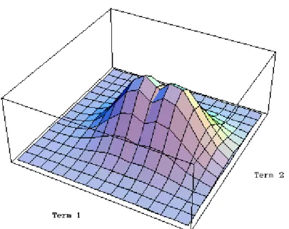
Our final experiment involved altering the patterns of covariance between terms in the simulations. Here we hypothesized that optimal k would change as we changed the type and the degree of term dependence. Specifically, we expected that more highly
conflation onto one or two LSI dimensions. Thus a termspace characterized by strong interdependence would be optimized at a fairly low dimensionality. Conversely, a dataset represented by independent terms would need a very high k to permit robust retrieval.
To test this hypothesis, we chose to model two degrees of term dependence. As discussed in Section 3, we altered term dependence by changing the covariance matrix used to parameterize the dataset's multinormal distribution. To keep our model simple we altered just two types of covariance: pairwise covariance and covariance for each term with non-adjacent terms (we refer to this as “distant” covariance). For our baseline test, each term had variance=.75 and covariance with each of its neighbors=.05. Thus termi and termi+/-1 share a correlation of r=.667 (see Appendix B "Sample Correlation Matrices"). This model is kept simple by assuming that termi shares no correlation with other terms. However, by association, termi and termi+/-2will share some variance by virtue of their correlation with termi+/-1. In non-baseline runs we altered the amount of pairwise covariance. In the following discussion "high" pairwise covariance refers to pairwise covariance=.35, while "low" covariance refers to covariance=.025.
Besides pairwise covariance, in one case we also modeled “distant” covariance. This was achieved by first assigning baseline pairwise covariance for a term. Next, all of the term's remaining variance was divided among the rest of the terms. Thus for a termi with .75 variance and .05 variance in a 300-dimensional termspace, all terms not adjacent to termi would share covariance=.002 with termi.
independence, and high pairwise covariance. Figure 11 shows the same iterations measured by mean precision. Both metrics show a similar trend. All three types of covariance provide roughly equal worst-case retrieval; at extremely low dimensionality all three retrieve at approximately 145 ASL and 55% mean precision. The three runs also display similar dynamics as k increases. Performance improves and then settles into an optimal plateau, or peaks in an optimal range of dimensionality.
Figure 10. Performance (ASL) in terms of shifting dimensionality for 3 types of term covariance
These plots support our contention that higher term correlation will lead to a lower optimal k. As we would expect, the highly correlated termspace reaches its plateau early on (at k > 50). The baseline run, with a small amount of pairwise correlation shows a dramatic range of optimal dimensionality near k=150. On the other hand, the
uncorrelated termspace never reaches an obvious plateau. Although it does show a steep improvement with the addition of the first few singular values, it continues to gain
discriminatory power throughout the range of its possible dimensions. According to the measurement by mean precision, the independent termspace does show a small
performance decline with the addition of the last few singular values. But over all, our hypothesis that term correlation should lower optimal k is borne out here.
Figure 12 shows retrieval performance for our baseline parameters, high pairwise covariance, and distant covariance. In step with our expectations, the more highly correlated termspaces (high pairwise, and distant) reach their optimal dimensionality early, at k >50, while the less highly correlated baseline data is optimized at k>200.
Like the termspace with high pairwise correlation the data modeled with distant correlation appear to support our hypothesis. Although they do not gain as much performance from dimensionality reduction as less highly correlated spaces, they reach their maximal dimensionality at a fairly low k value.
The results of our experiments with the type and degree of term covariance are provocative insofar as they lend evidence to the idea that dimensionality reduction and term dependence are related. The data presented here suggest that a highly correlated space will be optimized at a lower dimensionality than a weakly correlated space. For a highly correlated data set, the assumption of term independence inherent in the linear retrieval model is grossly wrong. Here LSI improves retrieval by reducing this error. That is, LSI works by improving the fit between the linear model and the non-linear data, by mapping the data onto the best possible linear space. For highly correlated data, the best possible space will be of relatively low dimensionality because the terms are quite similar and can thus be collapsed onto a single axis. In other words, highly correlated terms can be assumed to result from a single function. In a densely correlated space, only a few functions (or dimensions) are needed to describe the data points. On the other hand, in a weakly correlated space, most terms will be linearly independent of all other terms. Thus the retrieval model's assumption of term independence will not fit the data too badly. In this situation, LSI will need many more factors to describe the data.
the early portion of this discussion found several shortcomings in the type and degree of term dependence at work in our data. We will conclude this investigation, then, with an analysis of the relation between orthogonality and the SVD and how their relationship bears on our simulations.
6. Modeling Term Dependence: How Patterns of Covariance Affect
LSI
In the process of analyzing the simulation data, it has become clear that a more highly nuanced model of term dependence is necessary for a definitive study of the dynamics of LSI dimensionality reduction. What has become clear is that our simplified apparatus for altering term-term correlation does not provide an ideal dataset on which to test LSI. The essential problem that we have faced in the analyses reported here lies in the near
orthogonality of our simulated termspaces. This section describes how term dependence relates to orthogonality, and how this relation bore on our simulations.
Termspace Dynamics and SVD
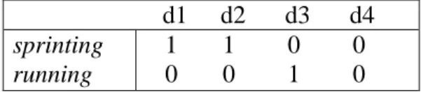
Consider the case of the tiny database illustrated in Table 2. The example shows a corpus of documents represented by orthogonal terms, driving and running.
d1 d2 d3 d4 sprinting
running
1 1 0 0 0 0 1 0
Table 8. A tiny corpus of documents represented in parallel termspace.
Figure 13. Singular values of orthogonal and parallel termspaces
Figure 13 shows the relationship between orthogonal and parallel termspaces graphically. Plotting the singular values of the data from Tables 2 and 8 the x-axis has the rank (first or second in this case), while the y-axis shows the singular value. The singular values of an orthogonal termspace generate a horizontal line. None of them are small, and thus we cannot benefit by removing them. In the case of the parallel
termspace, however, the difference between the first and second singular value is infinitely large. Graphically it appears as a constant slope (other graphing software would represent it as an L-shaped right angle).
nearly orthogonal the original termspace is. The closer a space comes to parallel term distribution, the lower optimal k is likely to be; a perfectly parallel termspace is
optimized for k=1. On the other hand, in a perfectly orthogonal termspace, optimal k would be equal to the full rank of the matrix A. Because few real termspaces are perfectly orthogonal or perfectly parallel, optimal k will fall somewhere between these two extremes.
Termspaces of the Simulated Data
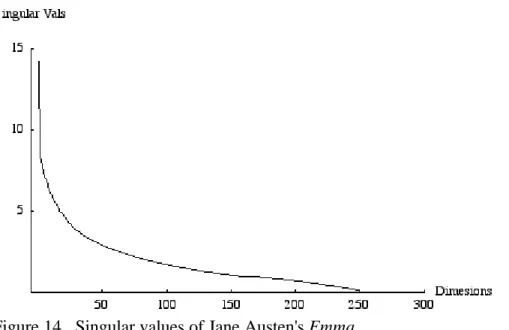
Figure 14 shows the singular values obtained by decomposing some real text6. The text is Jane Austen's Emma, divided into pseudo-documents that each consist of seven paragraphs (seven was chosen to make the rank of the matrix approximately equal to the baseline 300 used for our simulations). Because the text was segmented arbitrarily, the resultant singular values are probably a bit weaker than they would be for the case of semantic segmentation. Nonetheless, a very identifiable pattern emerges from this analysis.
The distribution of singular values seen here closely resembles the plots that Jiang and Littman, (forthcoming) made from several large corpora. Jiang and Littman suggest that singular values characteristically possess the so-called low-rank-plus-shift-structure. In other words, “the singular values are relatively large but decreasing sharply at the beginning, leveling off noticeably for the most part in the middle, and dipping again at the end” (Jiang and Littman, forthcoming). This characteristic bears on optimizing k because, “the dimensions that matter the most are the ones that correspond to the largest singular values,” (Jiang and Littman, forthcoming). Thus it is not surprising that several corpora that Jiang and Littman analyze level off between 100-200. This is also the case for Emma. These data suggest that kopt will lie in the vicinity of the “levelling off” of the singular values.
As the LSI factors begin to describe less covariance between term-document occurrences (as the singular values drop in size), adding them to the representation becomes useless. Optimal k, then, would be the first number whose associated singular value comes after the “levelling off” mentioned by Jiang and Littman.
Figure 15. Singular values for a dataset made with baseline parameters, and for Emma
In Figure 15 the largest simulated singular value has been omitted to make the scale of the graph legible. Thus the mean disjunction between the simulated singular values and those derived from Emma is even greater than it appears in this image. The first singular value derived from Emma is 14.2388, while the first from out baseline simulation is 119.601. The second singular value from Emma is 8.29545, while the second simulated value is 16.8749.
The discrepancy between simulated singular values and those derived from real data is disconcerting for two reasons. First, the very large ó1 in our simulated SVD suggests that almost all of the covariance in the original matrix is being captured by one dimension. This probably derives from dividing the documents into two discrete classes: relevant and non-relevant. Thus the spike seen at the head of Figure 15 is simply
The second problem evident in Figure 15 relates to the remainder of the simulated singular values. In the case of Emma, singular values 2-r are spread fairly widely:
(8.29545 - 1.76724 ‰ 1031 Þ 0). In constrast to this, the simulated singular values show much less dispersion: (16.8749 - 0.0199032). This means that the condition of our simulated matrices is highly suspect. Forsythe, Malcolm, and Moler (1977) define the condition of a matrix A by Formula 7.
cond(A) = ómax/ ómin (7)
In the case of an orthogonal matrix A, where all singular values are constant, cond(A)=1. Conversely, a parallel matrix(B) is said to have an infinite condition number because its ór will be 0 (in fact all of its sigmai, i¹1 would equal 0). If we disregard s1 because of the relevant/non-relevant problem discussed above, the condition for our simulated matrix is 847.8486. On the other hand, the condition for Emma is 8.05708 ‰ 10-31. By analyzing the condition of our simulated matrices it becomes clear that they are quite nearly orthogonal. Thus LSI has very little room for improvement upon them; for a matrix that is near to orthogonality, optimal k will be very close to the full rank of the matrix.
That a randomly generated matrix would not offer much in the way of patterns for LSI to captialize on is not surprising. What is surprising, though, is that our efforts to impose some pattern upon the randomness did not succeed. Our intent was to structure the simulated matrices by altering the covariance matrix that parameterized the
enough term dependence to make LSI more viable. In other words, we hoped to create matrices that violated the retrieval models assumption of linearity among the data. Appendix B ("Sample Correlation Matrices") shows that altering the covariance matrix did, in fact, alter the correlation between terms. The matrices resulting from models of term independence and high pairwise covariance are visibly distinct in their correlational structure. What is crucial, however, is that this distinction does not translate to decreased orthogonality of the data matrix. Table 9 shows that altering the correlation between terms does not alter the distribution of singular values.
Termspace First 10 Last
Emma {14.2388, 8.29545, 8.15617, 7.37346,
7.12835, 7.07342, 6.96749, 6.57713, 6.30498, 6.1465}
1.76724 ‰ 10-31
Baseline {119.601, 16.8749, 16.5007, 16.2433, 16.163, 16.0611, 15.8998, 15.8383, 15.7895, 15.6707 }
0.0199032
High pairwise
{121.013, 17.6701, 17.3728, 17.1004, 16.9426, 16.8637, 16.689, 16.5971, 16.3972, 16.2887 }
0.00044596
Term
independence
{ 119.711, 16.6362, 16.3927, 16.2185,
16.1081, 15.9207, 15.8666, 15.7112, 15.5579, 15.4154 }
0.0144299
Table 9. Distribution of Singular Values from Different types of matrix
Despite marked changes in their covariance matrices, all three simulated datasets produce very similar singular values. Moreover all three matrices share the defects described above: they have an exaggerated initial singular value, followed by a distribution of singular values that suggests near orthogonality.
7. Conclusion
Using multinormally distributed artificial datasets we tested the impact of a variety of variables on the dynamics of dimensionality reduction in latent semantic indexing (LSI). Our initial hypothesis was that optimal dimensionality reduction would depend on the correlation structure of the input term-document matrix. The vector-space retrieval model (of which LSI is a variant) assumes that terms occur in documents independently of the presence or absence of other terms. This is obviously not the case for most natural language texts. We have argued that LSI works by correcting this error.
Optimal dimensionality will depend on how badly the assumption of term
dependence is violated by a particular dataset. In a highly correlated termspace, LSI may map several terms with similar patterns of occurrence onto a single artificial factor. Thus such a termspace may be represented along a relatively small number of LSI dimensions. On the other hand, a space whose terms are nearly independent is already well fit by the linear language model assumed by the VSM. The best representation of such a dataset will be of a dimensionality near the matrix's full rank.
We found some evidence to suggest that adding terms and documents to a system inflates its optimal representational dimensionality. We hypothesized that adding terms and adding documents would lead to a non-monotonic increase in optimal k. Although our data offered only weak trends in this regard, these trends were encouraging.
Notes
1Manning and Scheutze (1999) suggest that a k value in the range of 50-150 should work
well. Dumais (1995), on the other hand, argues for a representational space near 300 dimensions.
2For a discussion of precision and recall, see Cleverdon (1967) Cleverdon (1972). ASL
is described in Losee (1998).
3
For a full discussion of the multinormal distribution, see Tong (1990).
4
The covariance matrix for these plots is described in Appendix 1 "Baseline parameters for simulations.”
5
See Appendix A "Baseline Parameter Settings" for a summary of these values.
6
References
Bartell, B. T., et al. (1992). Latent Semantic Indexing is an Optimal Special Case of Multidimensional Scaling. In Proceedings of the 15th Annual International ACM SIGIR Conference on Research and Development in Information Retrieval, Copenhagen, Denmark, pp. 161-167.
Cleverdon, C. W. (1967). The Cranfield Tests on Index Language Devices. Aslib Proceedings, 19, 173-192.
---. (1972). On the Inverse Relationship of Recall and Precision. Journal of Documentation, 23, 195-201.
Ding, C. H. Q. (1999). A Similarity-based Probability Model for Latent Semantic Indexing. In In Proceedings of the 22nd Annual Inter- national ACM SIGIR Conference on Research and Development in Information Retrieval, Berkeley, California, pp. 58-65, New York, ACM Press.
Dumais, S. T. (1995). Using LSI for information filtering: TREC-3 experiments. In D. Harman (Ed.), The Third Text Retrieval Conference (TREC3) National Institute of Standards and Tech- nology Special Publication, 219-230.
Berry, M. W., Dumais, S. T., and O'Brien, G. W. (1995). Using linear algebra for intelligent information retrieval. SIAM Review, 37(4), 1995, 573-595.
Deerwester, S., et al. (1990). Indexing by Latent Semantic Analysis. Jour- nal of the American Society for Information Science, 41(6), 391-407. Forsythe, G. E., Malcolm, M. A., & Moler, C. B. (1977). Computer
Methods for Mathematical Computations. Prentice-Hall, Engle- wood Cliffs.
Furnas, G. W., Landauer, T. K., Gomez, L. M., & Dumais, S. T. (1987). The Vocabulary problem in human-system communication. Communications of the ACM, 30(11), 964-971.
and Development in Information Retrieval, Berkeley, California, pp. 50-57, New York, ACM Press.
Jiang, F. & Littman, M. L. (Forthcoming). Approximate Dimension Equal- ization in Vector-based Information Retrieval. In Proceedings of the 17th Annual International Conference on Machine Learning, Stanford University.
Landauer, T. K. & Dumais, S. T. (1997). A Solution to Plato’s Problem: The Latent Semantic Analysis Theory of Acquisition, Induction, and Representation of Knowledge. Psychological Review, 104(2), 211- 240.
Landauer, T. K., Foltz, P. W., & Laham, D. (1998). Introduction to Latent Semantic Indexing. Discourse Processes, 25, 259-284.
Lochbaum, K. E. & Streeter, L. A. (1989). Comparing and Combining the Effectiveness of Latent Semantic Indexing and the Ordinary Vector Space Model for Information Retrieval. Information Processing and Management, 25(6), 665-676.
Losee, R. M. (1998). Text Retrieval and Filtering: Analytic Models of Per- formance. Kluwer, Boston.
Manning, C. D. & Scheutze, H. (1999). Foundations of Statistical Natural Language Processing. MIT press, Cambridge.
Oakes, M. P. (1998). Statistics for Corpus Linguistics. Edinburgh University Press, Edinburgh.
Project Gutenberg. (2000, Retrieved 30 March 2000). http://www.promo.net/pg/. Salton, G. & McGill, M. (1983). An Introduction to Modern Information
Retrieval. McGraw-Hill, New York.
Story, R. E. (1996). An Explanation of the Effectiveness of Latent Semantic Indexing by means of a Bayesian Regression Model. Information Processing & Management, 32(3), 329-344.
Tong, Y. L. (1990). The Multivariate Normal Distribution, Springer-Verlag. Van Rijsbergen, C. (1979). Information Retrieval (Second Edition).
Butterworths, London.
Wolfram, S. et al. (1999). Mathematica (version 4.0), Wolfram Research, Inc., http://www.wolfram.com.
Appendix A: Baseline Parameters for LSI Simulations
To provide a point of reference from which to judge the impact of shifts in LSI parameters, we defined the following baseline values for system variables. These values were chosen because during preliminary testing they gave results that left ample room for improvement in
performance without being so poor as to make any change in parameterization an improvement.
Parameter Value
Number of terms in the termspace 300
Variance for each term .75
Pairwise term covariance .05
Covariance for all non-adjacent terms (distant covariance) 0 Mean frequency of query terms in relevant documents .25
Mean frequency of all other terms .025
56
1 0.06667 0 0 0 0 0 0 0 0
0.06667 1 0.06667 0 0 0 0 0 0 0
0 0.06667 1 0.06667 0 0 0 0 0 0
0 0 0.06667 1 0.06667 0 0 0 0 0
0 0 0 0.06667 1 0.06667 0 0 0 0
0 0 0 0 0.06667 1 0.06667 0 0 0
0 0 0 0 0 0.06667 1 0.06667 0 0
0 0 0 0 0 0 0.06667 1 0.06667 0
0 0 0 0 0 0 0 0.06667 1 0.06667
0 0 0 0 0 0 0 0 0.06667 1
57
1 0 0 0 0 0 0 0 0 0
0 1 0 0 0 0 0 0 0 0
0 0 1 0 0 0 0 0 0 0
0 0 0 1 0 0 0 0 0 0
0 0 0 0 1 0 0 0 0 0
0 0 0 0 0 1 0 0 0 0
0 0 0 0 0 0 1 0 0 0
0 0 0 0 0 0 0 1 0 0
0 0 0 0 0 0 0 0 1 0
0 0 0 0 0 0 0 0 0 1