arxiv: v1 [math.na] 7 Jan 2021

TRANSFORM ON THE REAL LINE

CHRISTIAN KLEIN∗, JULIEN RITON, AND NIKOLA STOILOV

Abstract. A multi-domain spectral method is presented to compute the Hilbert transform on the whole compactified real line, with a special focus on piece-wise analytic functions and functions with algebraic decay towards infinity. Several examples of these and other types of functions are discussed. As an application solitons to generalized Benjamin-Ono equations are con-structed.

1. Introduction

We present an efficient numerical approach based on a multi-domain spectral method for the computation of the Hilbert transform on the real line. We are specifically interested in functions which are piece-wise analytic on_R, but we also discuss various other examples. The Hilbert transform of a function f ∈L2₍

R) is defined as (1) H[f](x) := 1 πP Z R f(y) x−ydy,

where P denotes the principal value. The Hilbert transform appears in countless applications in mathematics, physics and signal processing. Some important exam-ples include singular integral equations, see e.g. [18] where the Hilbert transform is used as the Cauchy integral on the real line. It is fundamental in linear response theory in the form of the Kramers-Kronig relations, for applications see [10]. Our main interest is in theory of water waves where the Hilbert transform appears for instance in the context of the generalized Benjamin-Ono (BO) equation,

(2) ut+um−1ux− Huxx= 0,

where m= 2,3, . . ., see [23] for a recent review and [22] for a numerical study. A convenient way to compute the Hilbert transform is via its Fourier transform, defined for a function f ∈L2₍

R) as

(3) fˆ(k) =Ff :=

Z

R

f(y)e−ikydy,

where k∈Ris the dual variable tox. It is well known that the Fourier symbol of

His simply given by

(4) F H=−isgn(k),

i.e., it is not smooth. With a Paley-Wiener type argument this immediately implies that the Hilbert transformH(f) cannot be rapidly decreasing inxfor|x| → ∞even

Date: January 8, 2021.

This work was partially supported by the ANR-FWF project ANuI - ANR-17-CE40-0035, the isite BFC project NAANoD, the ANR-17-EURE-0002 EIPHI and by the European Union Horizon 2020 research and innovation program under the Marie Sklodowska-Curie RISE 2017 grant agreement no. 778010 IPaDEGAN. We thank J.A.C. Weideman for helpful discussions and hints.

1

for functions f in the Schwartz classS(_R) of rapidly decreasing smooth functions because otherwise its Fourier transform would be smooth.

A standard numerical approach to compute the Hilbert transform is based on an approximation of the Fourier transform by a discrete Fourier transform (DFT). This is a spectral method, i.e., the numerical error in approximating analytic peri-odic functions decreases exponentially with the number NF of Fourier modes. In addition, the discrete Fourier transform can be efficiently computed with the fast Fourier transform (FFT) which is known to take O(NFlnNF) operations instead of the O(N_F2) the direct implementation of DFT takes. Thus, for functions in the Schwartz class, which can be seen as smooth and periodic on sufficiently large pe-riods within the finite numerical precision, such methods are highly efficient. The problem in the context of the Hilbert transform is the singular symbol (4) which, as mentioned above, implies that the Hilbert transform decreases only algebraically in 1/|x| for|x| → ∞. Such functions are not efficiently approximated via Fourier series.

Weideman [27] gave an elegant way to overcome these problems by introducing a mapping of the whole real line to the circle. This allows to take advantage of the efficiency of the FFT whilst avoiding the disadvantages of the approximation of Hilbert transforms via trigonometric functions in the integration variabley. The method, together with rigorous error analysis, is illustrated for several examples in [27]. There are many other numerical approaches for the computation of the Hilbert transform, see for instance [17] for a recent review and [4, 5, 21, 29] for new developments. Some of these approaches compute the Hilbert transform in terms of certain transcendental functions which then have to be computed as well. As we will show in this paper, for piece-wise analytic functions it is possible to compute the Hilbert transform in terms of elementary polynomials to the order of machine precision1_.

In this paper we address potential problems related to the mapping of the whole compactified real line to the sphere or a single interval. First, if the function of interest f is only analytic on a finite number of intervals In, n = 1, .., M, where ∪M

n=1In = R∪ {∞} and f ∈ Cr(R), r ≥ 0, a spectral approach will be only of

finite order on the whole real line, but of spectral accuracy on each of the intervals

In, n = 1, . . . , M. As an example of such a function Weideman [27] considers

f(y) = exp(−|y|) , which we will also discuss here. This function is also considered in [19] by mapping the half-lines R± separately. Second, a multi-domain method

offers the possibility to allocate resolution where needed. For instance for rapidly decreasing functions, no collocation points will be needed where the functions vanish with numerical precision.

Our multi-domain approach consists thus in mapping each of the intervalsIn,n=

1, . . . , Mto the interval [−1,1]. For infinite intervals we use 1/yas a local coordinate near infinity. The integrals are then computed with a spectral quadrature scheme as Clenshaw-Curtis [6]. For N collocation points in total the computational cost for the Clenshaw-Curtis quadrature is of the order O(N2_{/M) and thus of higher} complexity than Weideman’s FFT based algorithm, for the same total number

NF =N of collocation points used for his approach. However, we will show that for some of the examples of [27], a quadrature based approach is competitive as the total numberN of collocation points on all of the intervalsIn,n= 1, . . . , Mcan be

chosen much smaller than the NF necessary for in the Fourier approach and still achieve machine precision.

1_{Note, however, that the presented algorithm requires only piece-wise differentiable functions,} it is just most efficient for piece-wise smooth functions

The paper is organized as follows: in Section 2 we introduce our approach for functions which have an algebraic decrease for|y| → ∞. For the sake of simplicity we discuss in detail the case of two intervals. In Section 3 we discuss functions which are piece-wise analytic. In section 4 we address the case of functions with essential singularities at infinity. As an application of the approach, we construct solitary waves for generalized BO equations (2) in section 5. We add some concluding remarks in section 6.

Notation:

For clarity we establish the following convention: xis the external variable for the Hilbert transform,yis the internal, thusf generally is defined overyandH[f] is a function of x;k is the standard dual variable of the Fourier transform. The spaces in which x and y live normally coincide so if we e.g. integrate by parts we write

f(x) without further discussion.

2. _{Hilbert transform for functions analytical on the compactified}

real line

In this section, we consider functions with an algebraic decay for|y| → ∞. The approach is set up forNM domains, in generalNM−1finite ones and one infinite one. The choice of the number of domains is imposed by the problem we are studying. This means that if the function appearing in the Hilbert transform is piece-wise smooth (or at least C1 for our algorithm), say on NM−1 finite intervals, these intervals are a natural choice for the intervals in the method. In addition it can be that the conditioning of the integration scheme, for instance Clenshaw-Curtis, which is of the order ofO(N2

n), whereNn is the number of collocation points in the

interval In, see [24], becomes important if Nn has to be chosen large. As we will

later discuss in more detail, see also [6], the choice of Nn depends on the highest

Chebyshev coefficients since they are an indicator of the numerical accuracy (see the discussion of the examples). This means that the Chebyshev coefficients cn,

see (20), on each considered interval should be of the wanted order, say 10−16_{, for}

n ∼ Nn on each interval In. In cases where the number of collocation points in

the n-th interval Nn would have to be chosen too large (in practice much larger

than 100), it can be beneficial to subdivide this interval into several intervals such that each new Nn can be chosen small (in practice around 100). For the ease of

presentation, we discuss in detail below the case with two intervals one of which is infinite.

2.1. Finite intervals. We first address the case of a finite intervalIn = [an, bn],

. . . < an< bn< an+1< . . .,n≤NM−1. This means we consider the integral

(5) Hn(x) =P

Z bn

an

f(y)

x−ydy.

If x /∈In, the integrand of (5) is regular, and standard quadrature formulae could

be applied directly. If x∈ In, the principal value for x∈In can be computed in

classical manner, Hn(x) =P Z bn an f(y) x−ydy= Z bn an f(y)−f(x) x−y dy+f(x)P Z bn an 1 x−ydy = Z bn an f(y)−f(x) x−y dy−f(x) ln bn−x x−an . (6)

Note that the appearance of a logarithm in (6) does not imply that the Hilbert transform is unbounded since there will be similar terms from the other intervals

Inleading to a possibly regular expression on the whole real line (depending on the

regularity of f, see the example in subsection 2.2).

To compute the regular integrals in (5) or (6), we map them to the interval [−1,1] via y =bn(1 +l)/2 +an(1−l)/2, wherel ∈ [−1,1]. The integrals of the

form

(7)

Z 1

−1

g(l)dl

are computed with the Clenshaw-Curtis algorithm [6]: we introduce the standard Chebyshev collocation points

(8) lm= cos(mπ/Nn), m= 0, . . . , Nn.

Then with some weight functionswm, see [24] for a discussion and a code to compute

them, the integral (7) is approximated via

(9) Z 1 −1 g(l)dl≈ Nn X m=0 wmg(lm).

Thus for given weights wm, m = 0, . . . , Nn, this is just a scalar product. The

Clenshaw-Curtis algorithm is a spectral method, for an error analysis see [6]. We are interested in computing the Hilbert transform on the whole compactified real line. For convenience, we use the same discretisation inxas iny. Thus infinity becomes a finite point on our numerical grid. However, the Hilbert transform is not merely known on the collocation points inx. For intermediate points we apply a numerically stable and efficient interpolation algorithm in the form ofbarycentric interpolation, see [2] for a discussion and references. In this way we obtain the Hilbert transform not only at the collocation points, but for all x∈R∪ {∞}we

are interested in.

Ifx∈In, this can lead to an integrand with a limit of the type ‘0/0’. Assuming

that the function f is differentiable on In, this limit will be calculated via de

l’Hospital’s rule, (10) lim x→y f(y)−f(x) x−y =f 0_(y).

Remark 2.1. This formula shows also that the terms f(y_x)₋−f_y(x) appearing in our approach to compute the Hilbert transform are controled in standard way by the derivative f0(y) of the function appearing in the Hilbert transform. Since this derivative is by hypothesis finite, this controls the magnitude of the terms appearing in the quadrature routine.

The derivative off in (10) is approximated via Chebyshev differentiation matri-ces, see [24, 28],

(11) ~g 0(l)≈D~g(l),

where~g is the vector with the componentsg(l0), . . . , g(lNn), i.e., g sampled at the

Chebyshev collocation points. Since g is anyway sampled at these points, it is convenient to use a consistent differentiation method. For smooth functions and sufficiently small intervals, Nn can be chosen small enough so that cancellation

errors in the term f(y_x)−₋f_y(x) do not play a role. Note that the limit (11) could also be addressed via a deformation of the integration path near x into the complex plane (e.g., a small circle). However, since we are interested in applications related to dispersive equations as Benjamin-Ono, and since for such equations singularities in the complex plane can come close to the real axis, see [13, 11] and references therein, this is not a convenient approach in this context.

2.2. Infinite intervals. To treat infinite intervals, we use the local parameter

s= 1/yfory∼ ∞. We distinguish two cases, first where the functionf is analytic in s in a neighborhood of infinity, and second where this is not the case. In the first case we consider one interval of the form s ∈ [˜a,˜b], where ˜a = 1/a1 and ˜

b = 1/bNM−1, in the second case two intervals of the form s∈[˜a,0] and s∈[0,˜b]. Thus our approach can deal with functionsf which do not tend to the same finite value fory→ ±∞(in the latter case we would deal withNM−2finite intervals and two infinite intervals in total).

In both cases, we get an integral of the form (5)

(12) H∞= 1 xP Z ˜b ˜ a 1 sf(1/s) ds 1/x−s.

For the following discussion we assume that f(1/s)/s is bounded for s → 0, but this is not required in general. Note that we discuss in the following section how functions with an essential singularity at infinity can be treated. For the remainder of this section we assume that f is analytic in sfors∼0.

If 1/x /∈[˜a,˜b], the integral (12) can be computed as before with the Clenshaw-Curtis algorithm. If 1/x∈[˜a,˜b], we proceed as in (6):

(13) H∞= 1 xP Z ˜b ˜ a 1 sf(1/s) ds 1/x−s = 1 x Z ˜b ˜ a f(1/s)/s−xf(x) 1/x−s ds−f(x) ln 1/x−˜b 1/x−a˜ .

The simplest realisation of our approach is to compute the Hilbert transform on two intervals. For convenience we choose here y ∈[−1,1] and 1/y∈[−1,1]. This leads for (5) to (14) πH(f)(x) =P Z 1 −1 f(y) x−ydy+P Z 1 −1 f(1/s) s(x/s−1)ds. This is equivalent to (15) πH(f)(x) = Z 1 −1 f(y)−f(x) x−y dy+ 1 x Z 1 −1 f(1/s)/s−xf(x) s−1/x ds.

Thus the logarithmic terms cancel, and we are left with two integrals which are defined in a classical sense.

2.3. Examples. We illustrate the above approach with the example of a function which is analytic on _R∪ {∞}. Concretely, we consider the two functions

(16) f1(y) =

1

1 +y2, f2(y) = 1 1 +y4,

which are also examples one and two in [27]. The Hilbert transforms of both functions can be shown to be given in explict form

(17) H[f1](x) =− x 1 +x2, H[f2](x) =− x(1 +x2) √ 2(1 +x4₎. We generalize the first example of (17) slightly to

(18) f(y) = 1

a2_+y2, a∈R +_.

The Hilbert transform for this function can be calculated with (15) to give

(19) H[f](x) =− 2

aπ(arctan(1/a) + arctana) x a2_+x2, which gives for a= 1 the first result in (17).

We define as the numerical error err1the difference of the first integral in (15) for the function (19) and the explicit value 2/aarctan(1/a)x/(a2_+x2_{) forx∈[−1,1],} and err2 as the same difference for 1/x ∈ [−1,1]. ForN = 50 and a = 4, these errors are shown in Fig. 1. It can be seen that the error is for all values of xof the order of machine precision (10−16_here).

-1 -0.5 0 0.5 1 x -2 -1.5 -1 -0.5 0 0.5 1 1.5 2 err 1 10-16 -1 -0.5 0 0.5 1 1/x -4 -3 -2 -1 0 1 2 3 4 err 2 10-16

Figure 1. Difference of the first integral in (15) for the function

(19) fora= 2 andN = 50, on the left forx∈[−1,1], on the right for 1/x∈[−1,1].

To study the dependence of the numerical error on the number of points in each of the intervals, we define the error err as the L∞-norm of the difference between the numerically computed Hilbert transform and its exact value in both intervals. For simplicity we choose the same value of pointsN1,∞in both intervals, but this is not mandatory. The numerical error can be seen for the example (19) fora= 1 and

a= 2 and for the second example in (16) in Fig. 2. The spectral convergence of the code can be well recognized in a semi-logarithmic plot. The level of the rounding error is reached in the cases (16) for N1= 40 points, and for (19) witha= 2 with roughly 70 points. 0 20 40 60 80 100 N -16 -14 -12 -10 -8 -6 -4 -2 0 log 10 err 0 20 40 60 80 100 N -16 -14 -12 -10 -8 -6 -4 -2 0 log 10 err

Figure 2. L∞ norm of the difference between the computed

Hilbert transform and its exact value in dependence of the number

N1,2 of collocation points in each of the two intervals; the stars correspond to the example (19) for a = 2, the plus signs to the same function for a = 1 (example 1 of [27]), and the diamonds to the second case in (16) (example 2 of [27]); on the left with Clenshaw-Curtis, on the right with Gauss-Legendre quadrature.

Remark 2.2. The algorithm discussed above obviously does not depend on the use of Chebyshev collocation points. Instead one could use for instance Gauss-Lobatto points and apply Gauss-Legendre quadrature together with Legendre differentiation matrices for the terms of the form (10). The resulting errors are shown on the right of Fig. 2 for the same examples. As can be seen there is no advantage of the latter algorithm, which is in line with the discussion in [25]. We always use Clenshaw-Curtis in the following since we can compute the coefficients of an expansion in terms of Chebyshev polynomials efficiently (see remark 2.3).

Remark 2.3. It is evident that the error in the casea= 2 for function (19) decreases more slowly than in the casea= 1. Despite this, the error for y∈[−1,1] in Fig. 1 for N1,∞ = 50 is of the order of machine precision. These two facts indicate that it is not always optimal to choose the same number of points for both intervals. Thus one could either use intervals of the form x∈[−L, L] and 1/x∈[−1/L,1/L] with an optimized value ofL(this allows to use the same Clenshaw Curtis weights (9) in both cases) and the same number of points in both intervals, or the intervals as before with an optimized value of the number of collocation points for each interval. An indicator for such values can be obtained by considering in each interval the coefficients in an approximation of the function f via Chebyshev polynomials

Tn(x) := cos(narccos(x)), (20) f(x)≈ N X n=0 cnTn(x).

These coefficients can be computed efficiently via a fast cosine transform which is related to the FFT, see e.g. [24]. No fast algorithm is known for an expansion in terms of Legendre polynomials.

For the example (19), these Chebyshev coefficients are shown in Fig. 3. It can be seen that N1 = 30 points are sufficient on the finite interval to reach machine precision, whereas more than N∞= 80 are needed on the infinite interval.

0 20 40 60 80 100 120 n -20 -15 -10 -5 0 log 10 |cn | 0 20 40 60 80 100 120 n -20 -15 -10 -5 0 log 10 |cn |

Figure 3. Chebyshev coefficients for the example (19) fora= 2,

on the left for the interval [−1,1], on the right for the infinite interval.

2.4. Weideman’s approach to the computation of the Hilbert transform on the real line. As mentioned in the introduction, Weideman’s approach [27] is based on the mapping of the real line to the circle,

(21) y= tanθ

His approach uses an expansion of the considered functions in terms of rational functions

(22) φn=

(1 +iy)n

(1−iy)n+1, n∈Z,

instead of trigonometric ones: with (21) one obviously has that

(23) f(y) =X n∈Z anφn(y)⇒f(y)(1−iy) = X n∈Z aneinθ.

The Hilbert transform acts on the φnasHφn=isgn(n)φn,n∈Z, see [27]. On the

latter an FFT approach is implemented,

(24) f(y)(1−iy)≈

NF/2−1 X

−NF/2

aneinθ,

whereNFis an even natural number, and where the coefficientsan,n=−NF/2, . . . , NF/2− 1 are computed with an FFT. The Hilbert transform is thus approximated as

(25) H(f)≈ 1 1−ix NF/2−1 X n=−NF/2 isgn(n)aneinθ,

with the definition sgn(0) = 1. To approximate the Hilbert transform in this way, two FFTs are necessary. Note that we use here theNF as e.g. in [24] for the FFT, which is twice the value used in [27]. Since Weideman [27] compared his method to several numerical approaches, we will only relate our results to his in this paper.

The first example in (17) is trivial in this approach since f1(y) = (φ0(y) +

φ−1(y))/2 which also gives the formula for the Hilbert transform. The numerical errors in dependence of the numberNF in (24) for the second example in (17) and (19) are shown in Fig. 4 on the left. Spectral convergence is evident. The approach reaches machine precision with roughly the same number of points as used above in each of the two intervals, i.e., half the number of collocation points in total (an optimal choice would be N1+N∞ ∼110 compared to 80 points in Weideman’s approach). The values of NF needed to reach machine precision can be as usual estimated via the coefficients an, n=−NF/2, . . . , NF/2−1 which are shown on the right of Fig. 4.

0 20 40 60 80 100 n -16 -14 -12 -10 -8 -6 -4 -2 0 log 10 err -50 0 50 n -20 -15 -10 -5 0 5 log 10 |an |

Figure 4. L∞-norm of the difference between the computed

Hilbert transform (with the method [27]) and its exact value in dependence of the number nof collocation points on the left; the stars correspond to the example (19) fora= 2, and the diamonds to the second case in 16; on the right the coefficientsan for both

It is thus not a surprise that the approach [27] is somewhat more efficient for functions analytic on the whole real line. Still, the order of magnitude of the total number of collocation points to achieve machine precision is the same as for the Weideman approach and the multi-domain approach in the present paper.

3. Piece-wise analytic functions

Multi-domain spectral methods are especially efficient for functions which are not globally smooth, and this will be illustrated in the present section. We will address the example of two intervals as in the previous section, but with functions which are only continuous or not even that. Since the logarithms in formulae (6) and (13) are taken care of analytically, only the integrals there have to be computed numerically. These integrals have smooth integrands and can be efficiently computed. Note that the logarithms will lead to unbounded terms for functions which are not continuous onR.

Remark 3.1. For values ofxin the second interval, the integral in (6) over the first interval can be computed as in (5). But forxclose to the boundary of the interval, this leads to an almost singular integrand which is difficult to approximate with polynomials. This is why we insist here on piecewise analytic functions which allow for an analytic continuation of the function in the interval I1 to a slightly larger interval. The second line of (6) is used with this analytic continuation for xclose to the boundaries. In this way the integrand is always controlled by the derivative off.

Concretely we will address the example

(26) f = ( 1 a2 1+y2 , |y| ≤1 α a2 2+y2 , |y|>1,

where a1, a2, α are constants. Each function in the respective interval has an obvious analytic continuation to the whole real line. The Hilbert transform of (26) is with relations (6) and (13)

(27) H[f](x) = _a2 1arctan(1/a1) x a2 1+x2 +2_aα 2 arctan(a2) x a2 2+x2 − 1 a2 1+x2 − α a2 2+x2 ln 1−x 1+x .

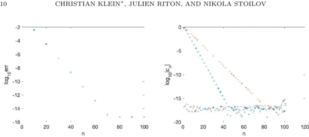
We consider first the case of a continuous potential, α= (a2₂+ 1)/(a2₁+ 1), where the Hilbert transform is bounded, and we choosea1= 1 anda2= 2. We use again the same numberN1,∞of collocation points in both intervals. The numerical error (as before, theL∞norm of the difference between numerical and exact solution) in dependence ofN1,∞can be seen on the left of Fig. 5. As expected the error decreases exponentially and reaches machine precision at essentially the same values as in the previous section. This means that as theoretically predicted, only the regularity on the respective intervals is important. As in the previous section, it is not optimal to choose the same resolution in both intervals. This is indicated by the decrease of the Chebyshev coefficients on the right of Fig. 5 for N1,∞= 100. They decrease in both cases exponentially, but more rapidly in the finite domain. Thus as in the examples of the previous section, N1+N∞∼120 would allow to achieve machine precision with two domains.

The situation is very different for the global approach [27] for which only the regularity on the whole compactified real line counts. The function (26) in depen-dence of the coordinate θ on the circle to which the real line is mapped can be seen on the left of Fig. 6. The corresponding coefficients an for this function can

Figure 5. L∞ norm of the difference between the computed Hilbert transform and its exact value (27) in dependence of the numberN of collocation points in each domain on the left; on the right the Chebyshev coefficients cn for both examples, the stars

corresponding to the finite interval, the plus signs to the infinite one.

be seen in the same figure in the middle. As expected for a piecewise continuous function, they only decrease algebraically, forNF = 1000 only to the order of 10−3. The difference of the numerical and the exact solution for NF = 1000 can be seen on the right of Fig. 6. It is of the order of 10−4 where the main error comes as expected from the domain boundaries where the function is not differentiable.

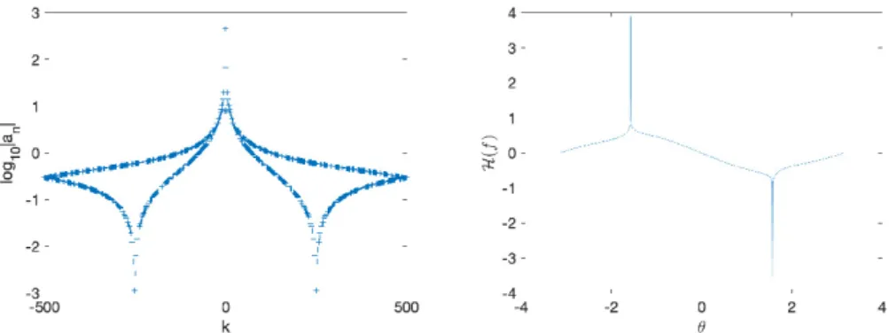
Figure 6. The function (26) in dependence of θ on the left, its

coefficents an in dependence of n for NF = 1000 in the middle, and theL∞ norm of the difference between the computed Hilbert transform (with the method [27]) and its exact value (27) forNF= 1000 on the right.

For discontinuous potentials being analytic on the respective intervals, not much changes for the multi-domain approach. If we consider the same example as in Fig. 5, just with α = 1, the error on the left of Fig. 7 shows virtually the same behavior as in Fig. 5. This is due to the fact the Chebyshev coefficients are the same up to multiplication by the factor α. As a function on the whole real line,f

is now obviously discontinuous, see the figure on the right of Fig. 7.

The discontinuity of f implies that the global approach [27] leads to a Gibbs phenomenon at the discontinuities, and the coefficients an consequently decrease

only very slowly, see the left of Fig. 8. The situation for the Hilbert transform is worse since the latter has a logarithmic divergence at the discontinuities as shown on the right of Fig. 8 (the values where the logarithm becomes infinite are obviously not shown). As is well known, logarithms are not efficiently approximated by Fourier series.

Figure 7. L∞ norm of the difference between the computed Hilbert transform and its exact value (27) in dependence of the number N1,∞ of collocation points in each domain on the left for the function shown on the right; on the right the function (26) in dependence of the coordinate θfora1= 1,a2= 2 andα= 1.

Figure 8. The coefficients an for the function on the right of

Fig. 7 for NF = 1000 on the left, and the Hilbert transform (27) on the right.

4. Essential singularities at infinity

The focus of this paper is on the Hilbert transform of functions which are piece-wise analytic on the compactified real axis. As has been shown in the previous sections for various examples, spectral convergence is achieved in such cases. For completeness we add here the remaining examples of [27] which have essential sin-gularities at infinity. The polynomial methods applied in the present paper are not ideal in such a case, but as we will show in this section, can still be used successfully. We first discuss the case of rapidly decreasing functions where the integration is just performed on finite intervals. We also add the case of oscillatory singularities at infinity for which deformation techniques are applied.

4.1. Rapidly decreasing functions. For rapidly decreasing functions, the main change with respect to the previous sections is that no integration on an infinite interval is needed. In the simplest case one just works on [−L, L] whereL >0 is chosen such thatf vanishes with numerical precision for|x|> L.

The first example in this context is example 5 of [27], the Gauss function with the Hilbert transform

(28) He−y2=−√2 πD(x), D(x) =e −x2 Z x 0 et2dt;

here D(x) is Dawson’s integral which we compute with the corresponding function in Octave (no tolerance is given there, but the results below indicate it is computed with machine precision).

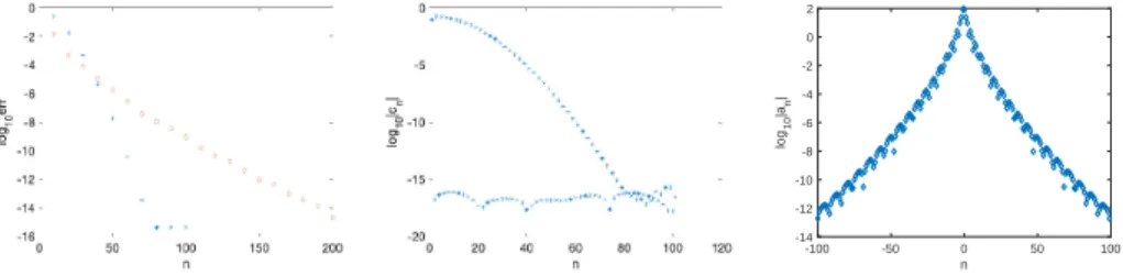
To compute the Hilbert transform of the Gauss function, we choose L= 6 (as usual in a way that the spectral coefficients decrease exponentially). The numerical error in the computation of the Hilbert transform can be seen on the left of Fig. 9. The error for the multi-domain approach (stars) decreases exponentially as expected and reaches machine precision with roughly 80 collocation points. In the same figure we show (diamonds) the corresponding error for the global approach [27]. Here around NF = 200 collocation points are needed to reach the same precision. This is obviously due to the essential singularity at infinity which is simply omitted (we work on a finite interval) in the multi-domain approach, but which is important in the global approach on the compactified real axis. This can be also seen from the spectral coefficients, in the middle of Fig. 9 for the Chebyshev coefficients of the multi-domain approach, and on the right of the same figure the coefficients of the expansion in terms of rational functions.

-100 -50 0 50 100 n -14 -12 -10 -8 -6 -4 -2 0 2 log 10 |an |

Figure 9. The numerical error for the computation of the Hilbert

transform for the Gaussian on the left (‘stars’ for the multi-domain method, ‘diamonds’ for the global approach), the Chebyshev co-efficients for the Gaussian in the middle, and its coco-efficientsan in

dependence ofnforN = 1000 on the right.

The situation changes somewhat if the function is just exponentially decreasing towards infinity, i.e., if the decrease is slower than for the Gaussian. Example 6 of [27] is the function sechxfor which the Hilbert transform is given by

(29) H[sech](x) = tanh(x) + i π ψ ₁ 4 + ix 2π −ψ ₁ 4− ix 2π ,

where the digamma functionψis given by the logarithmic derivative of the gamma function,ψ(z) =∂zln Γ(z). For the multi-domain approach we again use only one

interval which has to be much larger ([−40,40]) here because of the slower decay of the hyperbolic secans for |y| → ∞than the Gaussian. This also implies that with both the global and the multi-domain approach much higher resolutions are needed than in Fig. 9. The numerical error is shown on the right of Fig. 10. The global approach [27] reaches machine precision for roughly NF = 600 collocation points, the multi-domain approach for roughlyN= 900 points. This is in accordance with the spectral coefficients shown in the same figure in the middle and on the right respectively. This implies that in contrast to the case of the Gaussian, the global approach for this example is more efficient than the multi-domain approach.

Figure 10. The numerical error for the computation of the

Hilbert transform for the hyperbolic secans on the left (‘stars’ for the multi-domain method, ‘diamonds’ for the global approach), the Chebyshev coefficients for the function in the middle, and its coefficientsan in dependence ofnforN = 1000 on the right.

Example 7 of [27] is the functionf(x) = exp(−|x|), a rapidly decreasing function which is smooth onR±, but not onRand thus an interesting test for a multi-domain

approach. The Hilbert transform of this function reads

(30) H[e−|y|] =−1 πsgn(x) e|x|E1(|x|) +e−|x|Ei(|x|) , where E1(x) = Z ∞ x e−tdt t , Ei(x) =−P Z ∞ −x e−xdt t ,

i.e.,E1(−x) =−Ei(x)−iπ. For the multi-domain approach we use here 3 intervals, [−L,0], [0, L] and the infinite interval |x|> L. If we choose, as for the example in Fig. 10L= 40, the integral over the third interval vanishes with numerical accuracy. The integral on the interval [−L,0] for values of x∈ [0, L] can be regularized for

x ∼0 as in (6). This is problematic for some values ofx∈ [0, L] since exp(x) is exponentially growing in this interval. Therefore we use the regularization only for values ofx < L0 withL0∼1 (we takeL0= 1 here), and similarly for the integral over the interval [0, L] forx∈[−L,0].

The spectral coefficients for the multi-domain approach can be seen on the left of Fig. 11 (we show only the coefficients forx∈[−L,0] for symmetry reasons), and for the global approach [27] in the middle of the same figure. Machine precision is reached in the former case with just 40 collocation points, whereas in the latter the coefficients for N = 103 _{decrease to the order of 10}−3_{. The numerical error for the} multi-domain approach can be seen on the right of Fig. 112. It can be recognized that machine precision is reached with N ∼70 (the error for the global approach [27] for NF= 1000 is of the order of 10−4).

4.2. Oscillatory singularities at infinity. As stated the multi-domain spectral approach is intended for functions piece-wise analytic on the whole real line or with rapid decrease towards infinity. It has been shown for various examples that it works as intended in such cases. In the case of an oscillatory behavior at infinity as for examples 3 and 4 of [27],

(31) f1(y) =

siny

1 +y2, f2(y) = siny

1 +y4,

2_{The computation of the exact solution (30) is not trivial since the functionEi(x) computed} in Octave via the function expinthas to be multiplied with an exponential. Thus we write (30) in the formH(e−|x|_{) =−}1

πsgn(x) (Y(x)−Y(−x)), whereY =e

x_{Ei(x). The functionY satisfies}

the differential equationY0_{+Y = 1/xwhich is solved as in [7] on 3 intervals [−∞,−1], [−1,1],}

[1,∞] with the asymptotic condition limx→−∞Y = 0 and the substitutionY = ˜Y + lnxe−x in

Figure 11. The numerical error for the computation of the

Hilbert transform for the function f(x) = e−|x| _{on the left, the} Chebyshev coefficients for the function in the interval [−40,0] in the middle, and its coefficentsanin dependence ofnforNF = 1000 on the right.

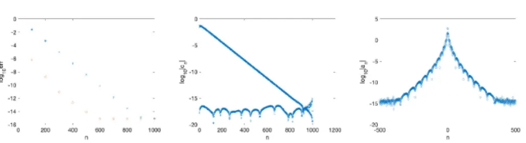
a spectral approximation is not ideal. We show the spectral coefficients both for the multi-domain approach in the infinite domain on the left and for the global approach [27] in the middle of Fig. 12. The algebraic decay of the coefficients in both cases can be seen.

Figure 12. The spectral coefficients for the functions (31) for NF = 1000, on the left the Chebyshev coefficients in the infinite domain |x| > 1, in the middle the coefficients for the global ap-proach [27], in blue forf1, in red forf2; the numerical error for the computation of the Hilbert transform for the functions (31) with a contour deformation approach are shown on the right.

The Hilbert transform for both functions is given by

(32) H[f1](x) = cos(x)−exp(−1) 1+x2 , H[f2](x) = cos(x)−exp(−1/ √ 2)(cos(1/√2)+sin(1/√2)x2) 1+x4 .

The error forNF = 1000 for the global approach is of the order of 10−3forf1and of the order of 10−7 _forf

2. To reach spectral convergence in such a case, deformation techniques in the complex plane appear to be necessary. Since the focus of this paper is on integration over the real axis (in order to be able to deal with functions for which the localization of singularities in the complex plane is not known), this is in principle beyond the scope of the current paper. But we add this example for completeness and to show how the techniques can be efficiently extended in this way. For the examples (31) we know that the singularities are, besides the obvious one on the real axis due to the Cauchy kernel, on the unit circle. Thus we can deform the integration contour from the real axis to y =eiα_{t+iβ, whereα, βare}

real constants and where t∈R. For an optimal choice of the deformed contours,

Instead of integrating the sine function, we consider integrals of exp(±iy) (or simply the imaginary part of the result for one of them) and choose for the first example in (31)α=±π/4,β=±0.5 and for the secondα=±π/8 andβ =±0.2. The signs are always chosen in a way that the integrand is exponentially decreasing towards infinity on the considered interval. In this way we have mapped the problem to the case treated in Fig. 11. We use the same parameters as there. Note that the terms proportional to cos(x) in (32) are the contribution of the residue of the Cauchy kernel on the real axis which is thus taken care off analytically. On the deformed contours, the integrands are regular and no regularization as on the real axis is needed. The numerical error for both examples can be seen on the right of Fig. 12. As expected spectral convergence is reached.

5. _{Solitary waves for generalized Benjamin-Ono equations} Benjamin-Ono equations (2) appear form= 2 in applications for instance in the modelisation of two-layer fluids, see [23] and references therein. The case m= 2 is in addition completely integrable. Form >2, the solutions to initial value problems with smooth localized initial data of sufficiently largeL2_{norm can have a blow-up} in finite time and are thus mathematically interesting, see [22] for a recent numerical study. As an application of the multi-domain spectral approach presented in the previous sections, we want to construct the solitary waves given numerically in [22] A solitary wave is a traveling wave solution of (2) vanishing at infinity, i.e., a solution of the form u(x, t) =Qc(x−ct) wherec >0 is a constant. Equation (2)

implies forQthe equation

(33) −cQc(ξ)−HQ0c(ξ) +

1

mQ

m

c (ξ) = 0,

where we have integrated the equation resulting from (2) once using the vanishing of Q at infinity; we have put ξ = x−ct to stress that (33) is a nonlinear and nonlocal equation in one variable only. In addition we have the scaling invariance

Qc(ξ) =cQ(cξ), where we have putQ(ξ) :=Q1(ξ). Thus it is sufficient to consider the case c= 1. The soliton in the integrable case m= 2 is explicitly known,

(34) Q(ξ) = 4

1 +ξ2,

the Lorentz profile we discussed in section 2 for the Hilbert transform.

To numerically construct the solitary waves form >2, we use the same approach as in section 2 with the two intervalsξ∈[−1,1] and 1/ξ∈[−1,1], and the same for the computation of the Hilbert transform. For simplicity we use the same number

N1,∞ of collocation points in both intervals for the integration in the variabley, but sample also ξon these points. Note that the Hilbert transform in the infinite interval is computed for the functionyQ(y). The derivative in (33) is approximated as before in terms of Chebyshev differentiation matrices. Thus we approximate (33) forc= 1 by the discrete nonlinear equation system

(35) F(Q) :=−Q−D_HQ+ 1

mQ

m_{= 0,}

where Qis the vector with components ofQ(ξn) withξn,n= 0, . . . ,2N+ 1 being

the Chebyshev collocation points in the two intervals, where _His the matrix cor-responding to the Hilbert transform, and whereDis the Chebyshev differentiation matrix as before. Thus we have to solve a nonlinear equation system which we do by a standard Newton iteration,

whereQ(k)_{is thekth iterate,k= 0,1,2, . . ., and where Jac is the Jacobian ofF(Q)} with respect toQ.

Note that the Jacobian has a kernel and thus cannot be inverted directly. This is partially due to a derivative appearing in the linear part of (33). To address this we require thatQis continuous forx=±1. Both conditions are implemented with Lanczos’τ-method [15]. In addition, equation (2) is translation invariant, ifQc(ξ)

is a solution so is Qc(ξ−ξ0) for constant ξ0. To fixξ0, we require thatQ0(0) = 0. This we implement numerically with a τ-method, to this end N1,∞ even in this section to make sure that ξ= 0 is a collocation point).

As the zeroth iterate we use in all cases A/(1 +x2), A > 0. The iteration is stopped once the L∞ norm ofF is smaller than some threshold, typically 10−10. Form >2 we use some relaxation to stabilize the iteration, i.e., in each step of the iteration the new iterate is formed byµQ(k+1)_{+ (1−µ)Q}(k)_{where 0< µ≤1.}

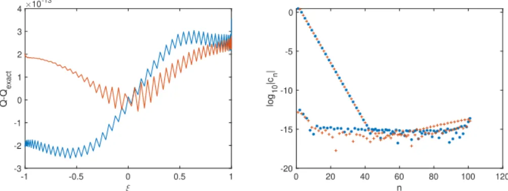
We first test the known solution for m= 2 with N1,∞ = 100. For A = 3,5 in the initial iterate, the Newton iteration converges after 5 iterations with a residual smaller than 10−10_{. The difference between numerical and exact solution can be} seen on the left of Fig. 13 to be of the order 10−13_{in both domains. The Chebyshev} coefficients of the solution in both domains on the right of the same figure indi-cate that N ∼50 collocation points are enough as in section 2 to reach maximal precision. -1 -0.5 0 0.5 1 -3 -2 -1 0 1 2 3 4 Q-Q exact 10-13 0 20 40 60 80 100 120 n -20 -15 -10 -5 0 log 10 |cn |

Figure 13. On the left the difference of the exact and the

numer-ical solution for the soliton form= 2, on the right the Chebyshev coefficients of the solution, in blue for the finite domain, in red for the infinite domain.

For higher values of m, we use N1,∞ = 300 collocation points in each domain. The solutions can be seen in Fig. 14 in the finite domain and are in accordance with [22]. The higher the nonlinearity, the more the solitary waves are compressed.

The solutions for larger m also require more numerical resolution, i.e., higher values of N in each domain as can be seen in Fig. 15. But forN1,∞ = 300, the coefficients decrease in all cases to the order of the rounding error.

Note that the solitary waves have the symmetry Q(−ξ) = Q(ξ). This is the reason why all odd Chebyshev coefficients in Fig. 15 vanish. To optimize resources, one could have worked on R+ only. But since we are in the future interested

in studying the dynamics of perturbations of the solitary waves, i.e., use Q plus perturbations as initial data for the generalized BO equation (2) as in [22], this is not convenient since the BO solution will not stay symmetric in general.

-1 -0.5 0 0.5 1 0 0.5 1 1.5 2 2.5 3 3.5 4 Q

Figure 14. The solitary waves of (2) form= 2,3,4 (from top to bottom).

0 50 100 150 200 250 300 350 n -20 -15 -10 -5 0 log 10 |cn | 0 50 100 150 200 250 300 350 n -20 -15 -10 -5 0 log 10 |cn |

Figure 15. The Chebyshev coefficients of the solitary waves for m= 3 on the left and form= 4 on the right, in blue for the finite domain, in red for the infinite domain.

6. _Outlook

In this paper we have presented a multi-domain spectral approach for the Hilbert transform on the real line. We have shown that it provides a comparable perfor-mance to Weideman’s global approach [27] for functions analytic on the whole real line. At various examples we have discussed that the global approach [27] based on an expansion in terms of rational functions is more efficient for functions with an algebraic decrease towards infinity, but that this can be slightly different for rapidly decreasing functions. In all cases the same order of magnitude of collo-cation points is needed to achieve the same accuracy. The FFT based approach [27] has a lower complexity and is thus the method of choice in such cases. The multi-domain approach is intended for piecewise analytic functions where it pro-vides spectral accuracy when a global approach is of finite order and may exhibit Gibbs phenomena. This was illustrated at various examples.

One application of the multi-domain approach will be to study zones of rapid modulated oscillations calleddispersive shock waves(see for instance [8] for a review with many references) which appear in the solutions of nonlinear dispersive PDEs as the Benjamin-Ono equation (2). A multi-domain approach allows a special

allocation of resolution where it is most needed, i.e., where the oscillations are. This is in particular interesting if one wants to study discontinuous initial data as in the case of the Gurevitch-Pitaevski [9] problem for the Korteweg-de Vries equation. Generalized BO equations (2) for sufficiently largepcan have solutions to initial value problems with smooth initial data which blow up in finite time, i.e., where the L∞ norm diverges, see [22] for a numerical study. The multi-domain approach will allow to study numerically such a blow-up with a combination of methods of [3] and a dynamical rescaling as for the generalized Korteweg-de Vries equations in [12]. This will be the subject of further research.

The multi-domain approach presented in the present paper was mainly developed for the real axis. However, as the example with an oscillatory singularity shows, it is straight forward to generalize this to arbitrary piecewise smooth contours in the complex plane. Each of the smooth arcs of such a contour (or parts of it) can be mapped to the interval [−1,1] where the same techniques as here can be applied to compute a Cauchy integral. The approach is also not limited to Cauchy integrals. In recent years, there has been an increasing interest in fractional derivatives, for instance in the context of PDEs with nonlocal dispersion, see e.g., [14, 16, 1]. The extent to which a multi-domain approach can be used to efficiently compute fractional derivatives will be studied in a separate work.

References

[1] L. Banjai, M. Lopez-Fernandez, Efficient high order algorithms for fractional integrals and fractional differential equations, Numerische Mathematik (2018) DOI: 10.1007/s00211-018-1004-0

[2] Berrut, J.-P. and Trefethen, L.N., Barycentric Lagrange interpolation, SIAM Review 46 (2004), 501-517.

[3] M. Birem and C. Klein, Multidomain spectral method for Schr¨odinger equations, Adv. Comp. Math., 42(2), 395-423 DOI 10.1007/s10444-015-9429-9 (2016)

[4] H.Boche and V. Pohl, Computing Hilbert transform and spectral factorization for signal spaces of smooth functions, ICASSP 2020 - 2020 IEEE International Conference on Acoustics, Speech and Signal Processing (ICASSP), Barcelona, Spain (2020), 5300-5304.

[5] M.C.De Bonis, B. Della Vecchia, and G.Mastroianni, Approximation of the Hilbert transform on the real line using Hermite zeros, Math. Comput., 71(239) (2001), 1169-1188.

[6] Clenshaw, C. W. and Curtis, A. R., A method for numerical integration on an automatic computer, Numer. Math. 2 (1960), 197-205.

[7] S. Crespo, M. Fasondini, C. Klein, N. Stoilov, C. Vall´ee, Multidomain spectral method for the Gauss hypergeometric function, Num. Alg., https://doi.org/10.1007/s11075-019-00741-7 (2019)

[8] T. Grava and C. Klein, Numerical study of the small dispersion limit of the Korteweg-de Vries equation and asymptotic solutions, Physica D, 10.1016/j.physd.2012.04.001 (2012).

[9] A. V. Gurevich and L. P. Pitaevskii, Nonstationary structure of a collisionless shock wave. Eksper. Teoret. Fiz. 65 (1973), no. 8, 5901-7604; translation in Soviet Physics JETP 38 (1974), no. 2, 2911-7297.

[10] S. H. Hall and H. L. Heck, Advanced Signal Integrity for High-Speed Digital Designs, Wiley Siclence (2009)

[11] RL James, JAC Weideman, Pseudospectral methods for the Benjamin-Ono equation, Adv. Comp. Meth. for PDEs 7, 371-377 (1992).

[12] C. Klein and R. Peter, Numerical study of blow-up in solutions to generalized Korteweg-de Vries equations, Physica D 304-305 (2015), 52-78 DOI 10.1016/j.physd.2015.04.003.

[13] C. Klein and K. Roidot, Numerical study of shock formation in the dispersionless Kadomtsev-Petviashvili equation and dispersive regularisations, Physica D, Vol. 265, 1–25, 10.1016/j.physd.2013.09.005 (2013).

[14] C. Klein and J.-C. Saut, A numerical approach to blow-up issues for dispersive perturbations of Burgers’ equation, Physica D: Nonlinear Phenomena (2015), 46-65, 10.1016/j.physd.2014.12.004

[15] C. Lanczos, Trigonometric interpolation of empirical and analytic functions, J. Math. and Physics, 17, 123-199 (1938)

[16] C. Klein, C. Sparber and P. Markowich, Numerical study of fractional Nonlinear Schr¨odinger equations, Proc. R. Soc. A 470: (2014) DOI: 10.1098/rspa.2014.0364.

[17] King, F.W., Hilbert Transforms: Volume 1, Cambridge University Press, 2009.

[18] Muskhelishvili, N.I., Singular integral equations, Groningen: Noordhoff (based on the second Russian edition published in 1946), 1953.

[19] S. Olver, Computing the Hilbert transform and its inverse, Math. Comp. 80(275), 2011, 1745-1767

[20] S. Olver, T. Trogdon, Riemann-Hilbert Problems, Their Numerical Solution, and the Com-putation of Nonlinear Special Functions, SIAM, Philadelphia, PA, 2015.

[21] V.Yu. Protasov, Approximation by simple partial fractions and the Hilbert transform, Izvestiya Math. 73(2) (2009), 333-349.

[22] S. Roudenko, Z. Wang, K. Yang, Dynamics of solutions to the generalized Benjamin-ono equation: A numerical study,preprint, arXiv:2012.03336

[23] J.-C. Saut, Benjamin-Ono and Intermediate Long Wave Equations: Modeling, IST and PDE, in Nonlinear Dispersive Partial Differential Equations and Inverse Scattering, ed. by P.D. Miller, P.A. Perry, J.-C. Saut, C. Sulem, Fields Institute Communications 83 (2019) [24] L. N. Trefethen, Spectral Methods in Matlab, SIAM, Philadelphia, PA, 2000.

[25] L.N. Trefethen, Is Gauss Quadrature Better than Clenshaw-Curtis?, SIAM REVIEW, 50, No. 1, pp. 67-87

[26] T. Trogdon, “Rational approximation, oscillatory Cauchy integrals and Fourier transforms”, Constr. Approx., 43, 71–101, 2016

[27] JAC. Weideman, Computing the Hilbert transform on the real line, Math. Comp. 64(210), 1995, 745-762

[28] Weideman, J.A.C. and Reddy, S.C., A Matlab differentiation matrix suite, ACM TOMS, 26 (2000), 465–519.

[29] C. Zhoua, L. Yang, Y. Liu, Z. Yang, A novel method for computing the Hilbert transform with Haar multiresolution approximation, Joru. Comp. Appl. Math. 223(2) (2009), 585-597 Institut de Math´ematiques de Bourgogne, UMR 5584, Universit´e de Bourgogne-Franche-Comt´e, 9 avenue Alain Savary, 21078 Dijon Cedex, France, E-mail [email protected]

Institut de Math´ematiques de Bourgogne, UMR 5584, Universit´e de

Bourgogne-Franche-Comt´e, 9 avenue Alain Savary, 21078 Dijon Cedex, France, E-mail [email protected] Institut de Math´ematiques de Bourgogne, UMR 5584, Universit´e de

Bourgogne-Franche-Comt´e, 9 avenue Alain Savary, 21078 Dijon Cedex, France, E-mail [email protected]