Implementing Subspace Identification on Shake Table
Model
Zoe Cooperband
June 20, 2017
Advisor: Peter Laursen
California Polytechnic State University, San Luis Obispo
1
Introduction
Subspace Identification (from here on out SI) is a field of applied mathematics that takes collected experimental time-history data and gives out information about the system that produced the data [6]. Another variant of Subspace Identification is Stochastic Subspace Identification (SSI), which only means that there was no input forcing function or white noise input, with only system re-sponse output is recorded. SSI is typically used in control analysis but here we apply the methods to the modal analysis of structures.
There are freely available SSI algorithms online that take in data and spit out system data [7]. This senior project didn’t involve theory - instead much of the work was in research behind how Subspace Identification works, implementing the algorithm in MATLAB, and applying the program to shake table data to validate the program. In other words, building the framework to make SSI a usable tool and practical learning experience for other undergraduate engineering students.
2
Motivation For SSI Use in Structural Applications
2.1
Pros and Cons
Traditional modal analysis techniques involve mass shakers which can be costly and troubling to move, or large and expensive shake tables. The structure is physically shaken with hydraulics or mass, which can be problematic for larger structures or structures with high damping. SSI algorithms can instead utilize ambient shaking to push a structure, gathering structural data with only accelerometers. While SSI based processes shouldn’t by any means be a replacement for tra-ditional analyses, but the strength of SSI is the simplicity and ease of the process. At the least, SSI provides a good ballpark estimate for structures [1].
SSI Analysis Traditional Analysis
Forcing: +Range of freq’s or ambient −Specific freq’s & time to resonate Modes Observed: +All modes and freq’s at once −Excited modes one at a time Damping: +All modes atonce −Snapback tests typically required Accuracy: −Unsure, need more info. +Good
Reliability: −−Largely untested ++ Tried, true, and recognized by code
properties assess damage. SSI can be useful because of it’s broad description of a structure and speed of data collection. Accelerometers can be left in a building and data continually downloaded for analysis - without engineers ever entering the building. This saves people from entering a po-tentially dangerous structure, as well as giving results back more quickly.
Another application of SSI is in redundancy and support of other analyses. With SSI, all fre-quencies are tagged, greatly decreasing the chance that an operator missed a mode. Also, torsional modes or other unpredicted structural irregularities may appear, suggesting further investigation. Finally, SSI can be a quick double-check that other analyses are on the right track. At the least SSI is a quick analysis that doesn’t require much investment to supplement other analyses.
3
Overview of How Subspace Identification Works
3.1
Framework
To understand SI, we first look at the framework within which SI operates. SI uses a common language in control theory: State Space. State Space can be described as a set of two differential equations and corresponding system matrices that dictate how a system will respond to any input function, and what information will be output [4].
˙
~
x(t) = A~x(t) +B ~f(t)
~
y(t) = C~x(t) +D ~f(t)
A, B, C, D System Matrices
~
f(t) Forcing Function ~
x(t) State Vector ~
y(t) System Response
("What you can sense")
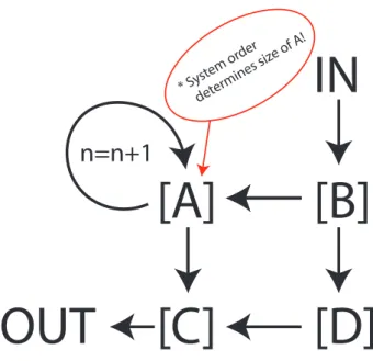
System Matrices A, B, C, D contain all the information of how the system will operate [4]. These four matrices fully determine and define the system. The forcing functionf~(t)is the only input into the system. For shake table models, this can be a single functionf(t), at the ground level corresponding to the direction of shaking. This response is "translated" through system ma-trixB, and effects state vector~x(t). Note, the state vector can be much larger or smaller than the input: in other words, the order of the system is independent of the input and output order.
System matrix A is where the focus of the SSI algorithm lies. Within an unforced system (stochastic),~x˙(t) =A~x(t)is a first order differential equation, and the structure outputs its nat-ural response of exponential growth/decay depending on the eigenvalues and eigenvectors of A [4]. MatrixA holds all information about the structural properties of whatever structure is being analyzed.
IN
[A] [B]
OUT
[C] [D]
n=n+1
* System or der
determines siz e of A!
Figure 1: Information Traveling Though State Space
3.2
The Process
State Space can readily replicate traditional analysis results. The typical engineering equation governing structural dynamics is given by:
M~y¨(t) +J~y˙(t) +K~y(t) =f~(t)
The translation to state space is given by [2]:
~ x(t) =
~ y(t)
˙
~ y(t)
A=
0 I
−M−1K −M−1J
B=
0
M−1
C=
I I
D=
0
With vector~y(t)being observed accelerometer time history data andf~(t)forcing at ground level.
The idea behind the SSI algorithm is, given~y(t)andf~(t)can we find system matricesA, B, C, D? The answer is yes, but only once we decide on what system order to make the internal state vector ~x(t)[2]. This can be arbitrarily small or large, but should be able to capture relevant information. On the later analyzed shake table model, 3 accelerometers were input into the algorithm. Since ~x(t)takes both velocity and displacement into account, this suggests a system order of 6 is needed to capture system dynamics. This number can (and should) be varied and experimented with.
is one method used to validate the written MATLAB program.
Once A is found, by SVD it’s decomposed [2]:
A= ΨΛΨ−1
Λ =
λ1 0 . . . 0
0 λ2 . . . 0
..
. ... . .. ...
0 0 . . . λn
HereΛ is the matrix of eigenvalues, which is then used to find [2]:
ωi=
ln(λi)
∆t
fi=
ωi
2π
ζi=
Re(λi)
|λi|
Φ =CΨ
Here,∆t is the time-step,fi is the frequency of modei,ζiis the damping of modei, andΦis the
modal matrix. For more details see [2]. Also, it is possible to find estimates of mass and stiffness matricesM andK(although one must be known to find the other) via:
M−1K= Φ
ω1 0 . . . 0
0 ω2 . . . 0
..
. ... . .. ...
0 0 . . . ωn
Φ−1
For a given system order n, n mode shapes and frequencies are output often with duplicate modes. To resolve this issue, duplicate modes are cut out. Another error arises from strong high-frequency modes that are introduced as a artifact of the algorithm – these modes are probably introduced from the discrete time steps jolting the data around. These modes should be trimmed away.
3.3
The Algorithm
What is missing from this explanation thus far is a description of the SSI algorithm itself. SSI uses lots of high-powered linear algebra that is, unfortunately, difficult to understand and explain. For more information, see [6] [3]
Briefly, the SSI algorithm projects different chunks of data at one time ti onto chunks from a
different timetj(in a sense averaging them) [3]. Over a range of time lagsti−tj, the corresponding
4
Implementing on Shake Table Model
4.1
The Set-Up
As a validation of the SSI program, accelerometer data from a shake table model was pushed through the program and compared to results found from traditional modal analysis. The tradi-tional analysis involved resonating the structure at specific frequencies. This other group was led by Karen, Carla and Jen, and worked in parallel with this project.
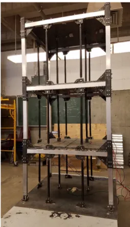
Figure 2: Shake Table Model
The model had 10 accelerometers attached, but for simplicity only 3 accelerometers (one at each floor and pointing in direction of forcing) were observed to find modes. El-Centro earthquake was used to force the structure. Surprisingly, SSI was able to find all mode shapes with a messy signal (that doesn’t cleanly rest at any frequency).
4.2
Results
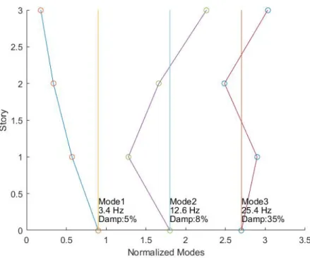
The SSI method was able to match the traditional analysis results almost exactly. The low 2-4% error can easily be from user estimation (since the frequencies were found by looking at the resonating structure for a maximum deflection). Additionally the Mode shapes line up perfectly.
SSI Results K & C Results % Error
Frequency 1 3.4 Hz 3.3 Hz 3%
Frequency 2 12.6 Hz 12.4 Hz 2%
Frequency 3 12.7 Hz 24.4 Hz 4%
Figure 3: Experimentally Found Mode Shapes
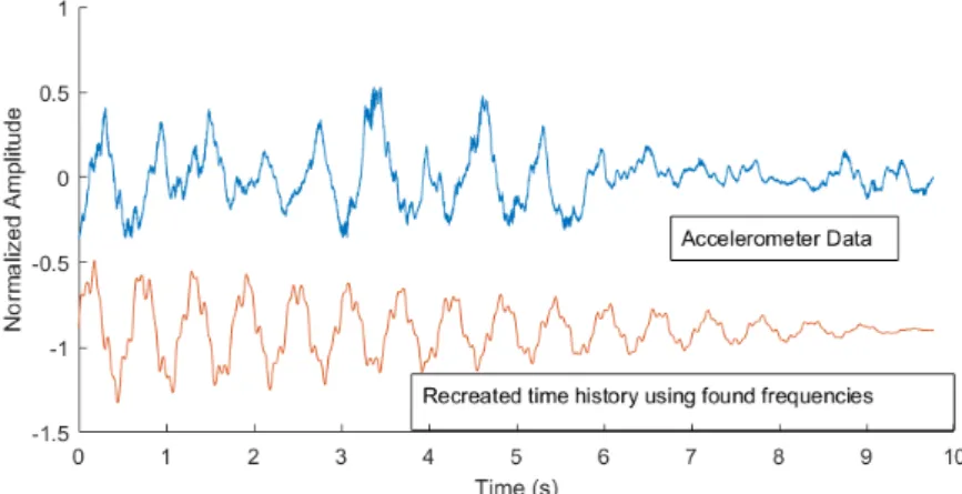
As a test, the found frequencies were used to roughly recreate the accelerometer data. In the following figure, the model is subjected to a impulse displacement (not El-Centro), while power from each mode and different damping is neglected. By no means is the resulting wave an accurate replication; this broadly shows the potential use of SSI in recreating realistic building behavior.
Figure 5: Sample Recreated Accelerometer Data
5
Conclusion
Stochastic Subspace Identification is a fast and valuable modal analysis technique. It’s easy to use and seems (initially) to give accurate results. There is good potential for use of SSI as a learning tool in the ARCE department as well as potential for future senior projects to investigate the process further.
Future potential topics of study include:
• Shake CM Building and analyze using SSI
• Develop method to find best system order
• Investigate using ambient shaking and white noise to collect data
• Combine and mix up selected input accelerometers (torsional modes?)
References
[1] S Adhikari. Structural dynamic analysis with generalised damping models: Identification.
[2] Rune Brincker and Palle Andersen. Understanding stochastic subspace identification. Proceed-ings of the 24th IMAC, St. Louis, Missouri, pages 279–311, 2006.
[3] Katrien De Cock, Bart De Moor, and KU Leuven. Subspace identification methods. Contribu-tion to secContribu-tion, 5:933–979, 2003.
[4] Bernard Friedland. Control system design: an introduction to state-space methods. Courier Corporation, 2012.
A
Matlab Code
%The following progam is a implimentation of a Stochastic Subspace
%Identification Algorithm on a Shake Table Model in the ARCE Seismic Lab. %Although the current Code is set to inport a specific set of data,
%modifications should be easily made to inport any other accelorometer data %set.
%This uses the Subspace Identification Toolbox written by Peter Van
%Overschee and BL De Moor. The key function used is subid, although another %versions of the program can be found in the toolbox. In the EXAMPLES %folder there are two tutorial programs to guide the user through %applications and instructions for using subid.
%Title: Implimenting Subspace Identification on Shake Table Model %Author: Zoe Cooperband
%Date: June 20, 2017 %Advisor: Peter Laursen %
%California Polytechnic State University, San Luis Obispo %Architectural Engineering Department
clc clear all
%---Importing Data & Variables---%
%The following code can be swapped for importing a specific dataset from %the home computer. Note that in a deterministic system (non-zero forcing), %the size of the input forcing array should be the same as the input
%data array with unused spaces filled with 0s.Here, there are 3 degrees of %freedom being observed.
addpath(’XXX\vanoverschee\SUBFUN’);
X=importdata(’XXX\ElCentro5SpanDapmpedX.mat’) Data=X.cordata;
Time=X.time;
%Organizing data Accel=Data(:,10); look=[2,5,8]; Ga=[0;0;1];
Degree=length(look);
View=zeros(size(Data,1),Degree); for i=1:Degree
View(:,i)=Data(:,look(i)); end
F=zeros(size(View)); F=(Ga*Accel’)’;
%Timestep: tj tj=1/2048;
%---End of User Input---%
[A,B,C,D,M,N] = subid(View,F,i,6); %SVD decomp
[V,P]=eig(A); SO=size(P,1); lam=zeros(SO,1); for i=1:SO
lam(i)=log(P(i,i))/tj; end
w=abs(lam);
%Frequency: fe fe=w/2/pi; %Damping: ze
ze=real(lam)./abs(lam);
%Trimming Duplicate and Extreme Modes wnew=[];
Vnew=[]; zenew=[];
for i=1:length(w)
if w(i) < 1/tj && w(i) > 1 %&& abs(ze(i)) < .5 if length(wnew) == 0 || abs(w(i)-wnew(end)) > 1
wnew=[wnew;w(i)]; Vnew=[Vnew,V(:,i)]; zenew=[zenew,ze(i)]; end
end end
fenew=wnew/2/pi;
%Transform Eigenvectors of A into Mode Shapes Cn=C*Vnew;
Mode=zeros(size(Cn,1),size(Cn,2)); numM=size(Mode,2);
W=zeros(length(wnew),length(wnew)); for i=1:size(Mode,1)
for j=1:numM;
Mode(i,j)=Cn(i,j) end
end
%Normalizing Modes ModeNorm=Mode; for i=1:numM
ModeNorm(:,i)=Mode(:,i)/norm(Mode(:,i)); end
zeSort(i)=zenew(IN(i)); end
%---Output---%
%Plotting Modes for Visualization figure
hold on for i=1:numM
dist=.9;
plot(dist*i+[ModeSort(:,i)’,0],[3,2,1,0]) scatter(dist*i+[ModeSort(:,i)’,0],[3,2,1,0]) plot(dist*i+[0,0],[0,3])
text(dist*i,1-.6,strcat(’Mode ’,num2str(i)));
text(dist*i,1-.6-.12,strcat(num2str(round(feSort(i),1)),’ Hz’))
text(dist*i,1-.6-.24,strcat(’Damp: ’,num2str(round(-zeSort(i)*100,0)),’%’)) end
xlabel(’Normalized Modes’) ylabel(’Story’)
hold off
%Output Final Modes & Frequencies Found disp(’ ’); disp(’ ’); disp(’Output: ’); disp(strcat(num2str(numM),’ modes’)); ModeSort
feSort
%The following is a possible method to extract stiffness matrix from %results:
% TestM=[100,0,0; % 0,100,0; % 0,0,50]; % SY=Mode*W*Mode^-1; % SY=SY^-1;