Predicting the Benefit of Rule Extraction A Novel Component in Data Mining
Tuve Löfström & Ulf Johansson
When performing data mining, the selection of data mining technique is a critical decision. Often this choice boils down to whether a transparent model is needed or not. Most research indicates that techniques producing trans-parent models, such as decision trees, often have an inferior accuracy compared to techniques such as neural networks. On the other hand, models created by neural networks are opaque, which must be considered a serious drawback as they are to be used for decision making. As an alternative, many researchers have tried to reduce this accuracy vs. comprehensibility trade-off by converting the opaque, high accuracy model into a transparent model – a technique termed rule extraction. In this paper, the question addressed is whether it is possible to predict, from the characteristics of a data set, if rule extraction is likely to produce an accurate model. The somewhat surprising answer, found from an empirical study conducted on several publicly available data sets, is that it is possible using only a few data set features. In addition, the study shows that the chosen representation is very important for the success of rule extraction. The results should be seen as steps in a direction towards a more automated data mining process. The overall ambition is to reduce the need for critical decisions having to be made early in the process and in an ad-hoc fashion.
Background
modeling or analyzing in mind, the collected data could contain potentially valuable information. Having a strategy for using the stored data to extract hidden information would typically be beneficial for a company or organization.
The activity of transforming collected data into actionable informa-tion, often termed data mining, is therefore increasingly becoming recognized as an important activity for companies as well as for other organizations. Although several definitions of data mining exist, they are quite similar. Berry and Linoff (1997, 5) use the following definition:
Data mining is the process of exploration and analysis, by automatic or semi-automatic means, of large quantities of data in order to discover meaningful patterns and rules.
The overall purpose of data mining is to support decision making by turning collected data into actionable information. A very rough sketch of the data mining process thus consists of data (input), the data mining activity itself, and information (output).
Data mining is used in many different domains so the nature of information found could be extremely varying. One typical example is a medical system where a diagnosis is suggested based on previous similar cases. Another example is a marketing system, where potential customers are mechanically selected for a promotion including an offer of a new service. The purpose of such a system could be to rank the recipients according to how likely they are to respond positively to the offer, leading to a targeted marketing effort. Obviously the system would use information on how the customers have responded previously to similar offers, if such data is available. More likely, though, the system would have to be built in accordance with the manner in which typical custom-ers have previously replied to comparable offcustom-ers. The problem is thus to find a general model.
At the same time, there is strong agreement among both researchers and executives about the criteria that all data mining techniques must meet. Most importantly, the techniques must have high performance. This criterion is, for predictive modeling, understood to mean that the technique should produce models that are likely to generalize well, thus showing good accuracy when applied to novel data. At the same time, the comprehensibility of the model is also very important, since the results should typically be interpreted by a human. Traditionally, most research papers focus on high accuracy, although the comprehensibility criterion is much emphasized by business representatives (see e.g. Berry & Linoff 2000).
In a description of an embryo to a standardized data mining method called CRISP-DM1 (The CRISP-DM consortium 2000), the advantage of having “a verbal description of the generated model (e.g. via rules)” is pointed out, thus acknowledging the importance of comprehensibility. Only with this description is it possible to “assess the rules; are they logical, are they feasible, are there too many or too few, do they offend common sense?”
It must be noted that the comprehensibility issue is tightly connected to the choice of data mining technique. Some techniques, such as decision trees and linear regression, are regarded as transparent,2
i.e. allo-wing human inspection and understanding. Other techniques, most notably neural networks, are said to be opaque and must be used as black boxes. However, these common descriptions are too simplified. Compre-hensibility, at least, also depends on the size of the model. For example, the comprehensibility of an extremely bushy decision tree is question-able.
With this trade-off in mind, several researchers have tried to bridge the gap by introducing techniques for converting opaque models into transparent models, while maintaining an acceptable accuracy. Most significant are the many attempts to extract rules from trained neural networks. This process of converting opaque models into transparent models is often called rule extraction.
Although the main purpose of rule extraction is to enable comprehensibility, and this normally leads to a loss of accuracy, an inte-resting question is whether the accuracy of the extracted model is higher or lower compared to a transparent model (e.g. a decision tree) generated directly from the data set. Many studies show that the extracted model in fact often has higher accuracy, when compared to the transparent model generated from the data set (see e.g. Dorado et al. 2002; Craven & Shavlik 1997; and Johansson, König & Niklasson 2004). If this was always true, there would be no reason to choose a less accurate technique just to obtain transparent models. A model created by a high accuracy technique, followed by rule extraction, would have higher performance (measured as accuracy and comprehensibility) than transparent models built directly from the data set.
It must be noted that this paper does not address the question of how to make sure that extracted representations are in fact comprehensible, although this is a very interesting topic. Naturally the argument used against bushy decision trees could be applied here as well. Transparency without comprehensibility is often of limited value in the data mining domain. Accordingly, we strongly believe that the ability to produce compact representations is a key property of any rule extraction algo-rithm. As a matter of fact, in our rule extraction algorithm G-REX, which uses genetic programming as extraction strategy, the accuracy vs. comprehensibility trade-off is explicitly handled to guarantee compact yet accurate rules. More specifically, the fitness function guiding the search includes components balancing accuracy and complexity. For details about G-REX see the original paper (Johansson, König & Niklas-son 2003).
the problem (both the data set and the task) determine which data mining technique is most suitable.
Much research in the metalearning community has been directed at finding techniques generally suitable for specific problem characteristics (see e.g. Kalousis, Gama & Hilario 2004; and Brodley 1994). In this research, many interesting and valuable findings have been made. Some of these results could be used directly in a general purpose tool, but some areas remain unexplored. One such area is to examine which types of data sets are suitable for rule extraction and which are not. Or put another way: is it possible for the data miner to know just from the characteristics of a data set whether rule extraction will increase the accuracy, compared to a transparent model generated directly from the data set?
Purpose and Motivation
The overall purpose of this study is to explore if it is possible to predict if a problem is suitable for rule extraction, by examining the characteristics of the data set. To determine if a data set is suitable for rule extraction, a comparison of accuracy is made between rules extracted from an opaque model (method 1) and rules created directly from the data set (method 2).
• Method 1: A high accuracy technique is used to produce an opaque model from the data set. Rule extraction is then performed on the opaque model to generate the final transparent model.
• Method 2: A transparent model is generated directly from the data set.
For each data set (and representation)3
a large number of model pairs are built using the methods described above. For each pair the most accurate model is deemed the winner. If a majority of winners come from Method 1, that data set (using that representation) is considered suitable for rule extraction.
Is it possible to mechanically determine, from the characteristics of the data set, whether rule extraction normally will produce a more accurate model, when compared to a model created directly from the data set?
Obviously this would be very beneficial since the choice of technique in that case would be more or less automated. More specifically, the accuracy vs. comprehensibility trade-off would be reduced and the suggested setup (a high accuracy technique followed by rule extraction) could be considered a good general-purpose data mining tool.
Data Mining
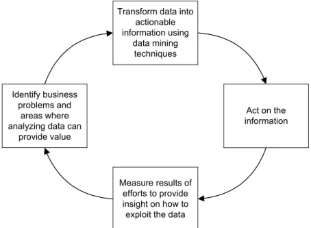
Data mining, as described above, is actually part of a larger process called the “virtuous cycle of data mining” (Berry & Linoff 1997), see Figure 1. To realize the full potential of the techniques, the data mining activity must be part of a company’s strategy, i.e. data mining should typically be considered as part of the customer-relationship management.
Transform data into actionable information using
data mining techniques
Identify business problems and
areas where analyzing data can
provide value
Act on the information
Measure results of efforts to provide insight on how to exploit the data
Whether the term “data mining” should be used for the entire virtuous cycle or just the “transform data into actionable information” step is a matter of taste, or more correctly, it depends on the abstraction level of the observer. In this paper, “data mining” mainly refers to applying different data mining techniques, but the business context and its demands are also recognized. More specifically, the fact that results from data mining techniques ultimately should be used by human decision makers places some demands on the data mining techniques themselves.
One particular and important demand, arguably also following from the fact that most business executives are still unfamiliar with data mining and data mining techniques, is that transparent models are preferred to black-box models. Black-box models are models that do not permit human understanding and inspection, while transparent methods produce explanations of their inner workings.
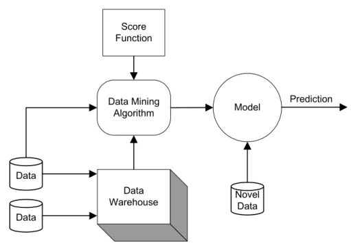
Data
Data
Data Warehouse Data Mining
Algorithm Model
Score Function
Novel Data
Prediction
Figure 2. Predictive modeling.
Most often a predictive model is found from directed data mining, i.e. a top-down approach where a mapping from a vector input to a scalar output is learnt from samples. The training data thus consists of pairs of measurements, each consisting of an input vector x(i) with a corresponding target value y(i). The predictive model is an estimation of the function y=f(x;θ) that can predict a value y, given an input vector of measured values x and a set of estimated parameters θ for the model f. The process of finding the best θ values is the core of the data mining technique. The two most important tasks for predictive modeling are classification and regression.
Predictive classification modeling deals with the case where the target is a categorical variable C. The target variable C is normally called the classvariable and takes values in the set {C1, C2,…,Cn}. Classification thus
consists of learning the mapping from an input vector of measurements x
referred to as features, attributes, explanatory variables and so on. Each feature can be real-valued, ordinal, categorical etc.
In predictive regression modeling the target is a real-valued variable. The problem is very similar to classification modeling, since the only difference is the numerical, rather than nominal, nature of the target variable. On the other hand, different measurements are used to deter-mine the accuracy of classification and regression models, i.e. the score functions are different.
It should be noted that the purpose of all predictive modeling is to use the model on novel data (a production set). It is therefore absolutely vital that the model is general enough to permit this. One particular problem is that of overfitting, i.e. when the model is so specialized on the training set that it performs poorly on unseen data.
Naturally, descriptive models and predictive models could (and often should) be used together in data mining projects. As an example, it is often useful to first search for patterns in the data using undirected techniques. These patterns can suggest segments and insights that im-prove the direct modeling results.
Learning Techniques
Many techniques for learning exist. The techniques described below are the techniques used in the experiments. The specific technique described in the section Strategies to increase generalization is a recent technique, inspired by existing methods for enhancing the generalization ability (for details see Löfström & Odqvist 2004).
Neural Networks
Artificial neural networks (ANNs) are highly parameterized models, loosely based on the function of the human brain. ANNs have proved to be successful in numerous data mining and decision support applica-tions, as well as in many other areas. ANNs are considered to be very powerful, general-purpose and readily applicable to predictive regression and classification.
units used and how they are connected) and a set of weights, i.e. how much adjacent neurons tend to activate or deactivate each other. The architecture is normally chosen before experimentation starts, but the weights are calculated during learning. For obvious reasons, this supervi-sed learning is often called training. The purpose of training is to adjust the weights to minimize the error function over the training set. There are many different learning algorithms for different architectures. Once the network is fitted to the training set, it may be regarded as a function mapping an input pattern to an output and could be used on novel data. If the ANN is good at generalization, it should produce reasonable outputs when presented with previously unseen input patterns. For a more detailed description of Neural Networks, see any introductory text, e.g. Haykin 1999.
Decision Trees
Decision trees is a predictive modeling technique most often used for classification. Decision trees partition the input space into cells where each cell belongs to one class. The partitioning is represented as a sequence of tests. Each interior node in the decision tree corresponds to one test of the value of some input variable, and the branches from the node are labeled with the possible results of the test. The leaf nodes represent the cells and specify the class to return if that leaf node is reached. The classification of a specific input tuple is thus performed by starting at the root node and, depending on the results of the test, following the appropriate branches until a leaf node is reached.
cell contains tuples from one class only. At the same time, the decision tree must not simply memorize the training set, but should be capable of generalizing to unseen data, i.e. the decision tree should not overfit. The goal is thus to have a decision tree as simple (small) as possible, but still representing the training set well.
Two basic strategies for avoiding overfitting is to stop growth of the tree when some criterion has been met, or to afterwards reduce (prune) a large tree by iteratively merging leaf nodes.
Classification and regression trees (CART) (Breiman et al. 1984) is a technique that generates binary decision trees. Each internal node in the tree specifies a binary test on a single variable, using thresholds on real and integer-valued variables and subset membership for categorical variables. Entropy is used as a measure for choosing the best splitting attribute and criterion. The splitting is performed on what is determined to be the best split point. At each step, an exhaustive search is used to determine the best split. For details about the function used to determine the best split, see Breiman et al. 1984. The score function used by CART is misclassification rate on an internal validation set. CART handles missing data by ignoring that tuple in calculating the goodness of a split on that attribute. The tree stops growing when no split will improve the performance. CART also contains a pruning strategy which can be found in Kennedy et al. 1998.
Cross Validation
As mentioned above, an important problem when creating models by learning from a data set, is the risk of overfitting. If a neural network or decision tree is allowed to learn the training data too well, it will not be able to generalize properly to unseen data. To avoid this, a statistical tool called cross validation is often used. When cross validation is used, the data set is divided into three disjoint subsets:
• training subset (used to train the model)
• validation subset (used to test or validate the model while training)
Cross validation is normally performed by repeatedly evaluating the current model against the validation set during training. When training has reached a certain point, it begins to learn details specific to the training data. Up to that point the validation error decreases, but when learning of overly specialized details in the training data begins, the validation error will start to increase. If training is stopped at the correct time (i.e. just before the validation error starts to increase) the result is a model likely to generalize well.
It should be noted that the generalization performance is ultimately measured on the test set. If the accuracy on the test set is close to that of the validation set, this is a strong indication that the model is general enough.
When there are few instances in the data set, multifold cross-validation is often a good solution. The basic idea is to estimate how well a model will predict unseen data. This is done by setting aside some fraction of the data and using it to test the prediction performance of the model generated from the rest of the data. K-fold cross-validation means that k experiments are run, each time setting aside 1/k of the data to test on. The final result is the average from the experiments. This is a standard procedure having the additional benefit of making results from different studies (using common data sets) comparable.
A special case of the multifold cross validation is called leave-one-out cross validation. When leave-one-out cross validation is used, k is set to be equal to the number of data points, i.e. there are as many experiments as there are data points and in each experiment only one data point is used as test set.
Strategies to Increase Generalization
contain some valuable information, and use of this information will produce a more general model.
The generalization strategy used in this study was developed by Löfström & Odqvist (2004), and is a variant of the generic strategy described above. Here the subset used for training is fixed and selected in advance. The remainder is used as a validation set. A trained model is evaluated against the validation set after each training. Instances incorrec-tly classified are moved from the validation set to the end of the training set. At the same time, an equally sized set of instances is moved back from the beginning of the training set to the validation set before the model is retrained. This is repeated until all the instances in the validation set are correctly classified or a selected number of iterations have been completed.
Committee Machines
This section presents different methods for combining several so called experts (neural networks, decision trees, or some other kind of learning algorithms) to reach a better overall decision. Such combinations of experts are called committee machines, a common tool to obtain more general models. A brief description of ensemble methods and boosting methods is presented below.
Ensemble Methods
The experts in ensembles could be homogeneous (like a set of neural networks) or a collection of experts using different learning algorithms, for instance neural networks and decision trees together.
Boosting
The experts in ensembles are trained on the same set of data. In a boosting machine, the experts are trained on data sets with different distributions. Boosting can be used to improve the performance on any learning algorithm. The original idea of boosting was described by Schapire (1990) and was called boosting by filtering. In boosting by filtering, the committee machine consists of three experts or sub-hypotheses. The first and second experts are trained on disjoint sets of training data. The third expert trains on a third training set that is built by selecting only those instances that the first and second experts disagree on.
When the boosting committee machine is evaluated against unseen data, it can draw its conclusions either by voting or averaging. The voting in boosting by filtering committee machines is performed in much the same way as the filtering of the third set. If both the first and second experts agree, that class label is used, otherwise the class label discovered by the third expert is used.
A very common technique, suggested by Freund & Schapire (1996) is called AdaBoost. The AdaBoost algorithm combines the predictions of several weak classifiers (i.e. a classifier with hypothesis slightly better than random guessing) into one with very good accuracy. For a detailed description of the algorithm see the original paper.
Rule Extraction
As described in the introduction, the purpose of rule extraction is to transform an opaque model into a transparent model. Rule extraction is typically performed using one of two strategies, called black box and open box.
from any kind of committee machines. An open box technique, when applied to a neural network, typically works by extracting rules for each layer and finally combining these rule sets into one rule describing the model the neural network has created. The way different methods create their local rules for each layer differs, but typically the weights of each layer are used in some way to create the rules. The RX algorithm by Lu, Setino & Liu (1995) is a typical example of an open box rule extraction algorithm.
A rule extraction technique using the black box strategy, on the other hand, directly creates a function describing the output in terms of the input. Typically some symbolic learning algorithm is used on the train-ing examples generated by the opaque model, i.e. the purpose of the rule extraction algorithm is to find and express the function between input and output learned by the opaque model, see Figure 3.
Data
Data Mining Algorithm
Opaque Predictive
Model Score
Function
Novel Data
Prediction Rule
Extraction Algorithm
Score Function
Extracted Predictive Model
Figure 3. Black box rule extraction.
mapping input to output (expressed in original variables) could be regarded as a black box rule extraction technique. With this viewpoint, decision tree algorithms like CART could be used for rule extraction, even though they are not originally intended for that use.
Meta Learning
Meta learning is concerned with the task of discovering general insights about different problems and learning techniques. Several previous studies have compared many learning techniques on numerous problems and analyzed the results from different angles (see e.g. Lim, Loh & Shih 2000). Most studies have focused on the relative performance of the learning techniques, but Kalousis, Gama & Hilario (2004) go one step further when they try to find similarities between both learning techniques and data sets. Brodley (1994) shows in her dissertation that different learning techniques are superior for different problems.
Characteristics of Data Sets
All data sets have a number of characteristics that can be represented in different ways. Among those characteristics are:
• the number of classes and the distribution of instances in these classes
• the number of instances
• the number of categorical variables
• the number of continuous variables
• the total number of variables
• some kind of measure of how much each variable contributes to explain the output
Characteristic Symbol
Lg # Instances LgI
Lg (# Instances / # Variables) LgRIV
Lg (# Instances / # Classes) LgRIC
% of Symbolic (Categorical) Variables PSV
% of Missing Values PMV
Class Entropy CE
Normalized Class Entropy NCE
Median of the Uncertainty Coefficient MedUC
Table 1. Data set characteristics
Similar characteristics have been suggested by Michie, Spiegelhalter & Taylor (1994), and have been used in other studies, e.g. Gama & Brazdil 1995.
Data Representation
The data can be represented in several different ways. The chosen repre-sentation plays an important role when training. As a matter of fact, a problem domain can often be represented in several different ways. One real-world example where the representation makes a difference is the problem of finding genes in DNA. Craven & Shavlik (1995) showed that the way the domain knowledge about genes is coded did make a difference. Their study showed that when the input was coded as nucleotides it was much harder to obtain good accuracy compared to input coded as codons.
Even without domain knowledge, data can be represented in different ways. The most obvious example is that individual variables (both conti-nuous and categorical) can be coded in different ways.
We will present a few ways of representing data that are possible to use for all categorical and continuous variables. The different represen-tations all split a single variable into several new variables that represent the original variable. By using more variables to represent the data set, learning techniques might find it easier to identify and learn interesting combinations of values.
Often categorical data is represented by different classes, each with a unique identifying label or number. An alternative way of representing categorical data is to divide it into as many binary variables as there are classes. Each binary variable will thus represent one class.
technique might lead to loss of information. A more complicated technique, to avoid this loss of information, is to find dynamic intervals, tailored for the specific problem.
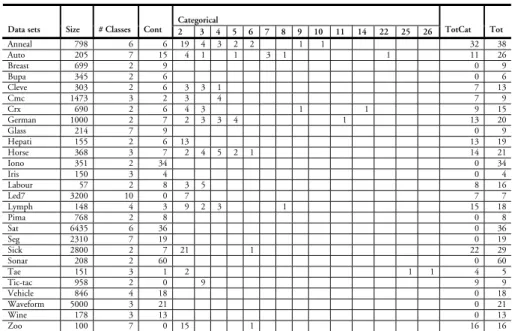
Data Sets
The data sets used in this study are all publicly available and were gathered from the UCI Repository (Blake & Merz 1998), see Table 2.
Categorical
Data sets Size # Classes Cont 2 3 4 5 6 7 8 9 10 11 14 22 25 26 TotCat Tot
Anneal 798 6 6 19 4 3 2 2 1 1 32 38 Auto 205 7 15 4 1 1 3 1 1 11 26 Breast 699 2 9 0 9
Bupa 345 2 6 0 6
Cleve 303 2 6 3 3 1 7 13
Cmc 1473 3 2 3 4 7 9
Crx 690 2 6 4 3 1 1 9 15
German 1000 2 7 2 3 3 4 1 13 20 Glass 214 7 9 0 9 Hepati 155 2 6 13 13 19 Horse 368 3 7 2 4 5 2 1 14 21 Iono 351 2 34 0 34
Iris 150 3 4 0 4
Labour 57 2 8 3 5 8 16 Led7 3200 10 0 7 7 7 Lymph 148 4 3 9 2 3 1 15 18
Pima 768 2 8 0 8
Sat 6435 6 36 0 36 Seg 2310 7 19 0 19 Sick 2800 2 7 21 1 22 29 Sonar 208 2 60 0 60
Tae 151 3 1 2 1 1 4 5
Tic-tac 958 2 0 9 9 9 Vehicle 846 4 18 0 18 Waveform 5000 3 21 0 21 Wine 178 3 13 0 13 Zoo 100 7 0 15 1 16 16
Table 2. Description of data sets
Method
Since the chosen representation might influence the suitability of rule extraction, two different representations were evaluated in this study. The first representation, called Original, used all input data in the form it was originally represented. The second representation, called Recoded, used input data recoded into binary form. The continuous variables were divided into 10 equal sized intervals prior to the transformation into binary form.
When selecting the learning techniques, some criteria had to be applied. Since the study aims at investigating the general question of whether it is possible to predict if a data set is suitable for rule extraction, learning techniques that would perform well on many data sets were needed. The selected techniques range from single neural networks and decision trees to different forms of committee machines, including ensembles and boosting machines. The range is believed to represent both more common as well as more specialized learning techniques.
The selected learning techniques are presented in Table 3. The selected learning techniques will be referred to as the techniques in the succeeding text.
# Name # Experts Type of Expert
T1 Committee 5 Neural network
T2 Cross validation committee 5 Neural network T3 Boosting by filtering 3 Committee of 3 neural networks T4 Generalization committee 5 Neural network
T5 Decision tree 1 CART
T6 Neural network 1 Neural network
Table 3. Techniques used in experiments
Basic Setup
The basic setup was equal for all data sets and consisted of two phases described in the two following sub-sections.
Comparing Rule Extraction with Transparent Techniques
Each data set was initialized so that two representations of the data set were created. Each data set representation was divided into three sets: a training set (including an early stopping validation set), an independent validation set and a test set. Fifty cycles of training were performed. Every cycle operated on a unique distribution of data, i.e. all three sets were rearranged for every cycle. In each cycle, the two representations of the data set were trained with all six methods, resulting in 12 trained models, see Table 4.
R1+T1 R1+T2 R1+T3 R1+T4 R1+T5 R1+T6 R2+T1 R2+T2 R2+T3 R2+T4 R2+T5 R2+T6
Table 4. Scheme of trained models in a cycle
Each of the 12 models in a cycle produced a predicted output. The predicted output and the original output were used to compare the model and the data. The comparison was performed as follows:
1. Train a model on original output with CART and save the result. (TransparentAcc)
2. Train a model on predicted output with CART and save the result. (ExtractionAcc)
Analyzing Data Set Characteristics
When phase one was finished for all data sets, the second phase began. Each data set was analyzed and the criteria for each one were measured. All the criteria mentioned in the section on Characteristics of data sets were used (except PMV due to lack of information about missing data for some of the data sets). PSV, LgRIV and medUC varied for the different representations of each data set. At the same time as these criteria were calculated, a dependent variable, i.e. output, was also calculated.
When calculating the output, comparisons between each pair of extracted model and transparent model were carried out, using the ExtractionAcc and TransparentAcc described above. If ExtractionAcc was higher than TransparentAcc, then the opaque model from which the extraction was done was considered a suitable model.
As a consequence of the definition of a suitable data set (see Purpose and motivation), those representations4 with more than 50 % of suitable models were considered suitable for rule extraction. The output was set as a binary variable where all suitable data sets were represented as 1 and all unsuitable data sets as -1.
As a result of the second phase, 27 instances of data for each repre-sentation, describing each data set, had been created.
Two different sets of output were created for each representation. The first only considered the best opaque model per cycle for a particular representation (measured on the validation set), resulting in 50 models per representation. In the second set all models were considered, i.e. 300 models, 50 cycles and models from 6 methods in each cycle. They will be called, respectively, the best selection and all models.
Predicting Data Sets Suitable for Rule Extraction
The actual prediction of whether or not a data set is suitable for rule extraction, could obviously be done in several ways. To make the model easy to interpret, CART was again chosen as learning technique. CART was used with the default settings as implemented in Matlab 7.0. The only parameter that was altered was the minimum split condition.
with the leave-one-out cross validation technique; i.e. for each data set, the meta information for all but the actual data set were used to train a decision tree, which was then evaluated on the remaining data set. If a suitable data set was predicted to be suitable, or an unsuitable data set was found to be unsuitable, the prediction was deemed correct.
Results
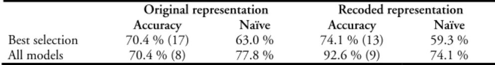
Table 5 shows the results from the prediction of whether or not a data set is suitable for rule extraction.
Original representation Recoded representation
Accuracy Naïve Accuracy Naïve
Best selection 70.4 % (17) 63.0 % 74.1 % (13) 59.3 % All models 70.4 % (8) 77.8 % 92.6 % (9) 74.1 %
Table 5. Summary of results from data set prediction
The values in parenthesis were the minimum split value used for that specific result. The naïve guess (the majority guess) was unsuitable, i.e. most of the data sets were not suitable for rule extraction.
Problem Analysis
As can be seen, there are some differences between the two represen-tations. The original representation resulted in fewer suitable data sets compared to the recoded representation. It is also harder to predict the suitability using the original representation. For the recoded represen-tation the predictions are rather good, while the results for the original representation are much worse. The result on all models using the original representation is even worse than the naïve guess.
It should be noted that for a data miner the best selection is probably the most interesting, since some choice of model, based on accuracy, is always used.
Criteria Analysis
criterion was evaluated from the number of times it was used to split the root node, the nodes in the second layer and in the third layer.
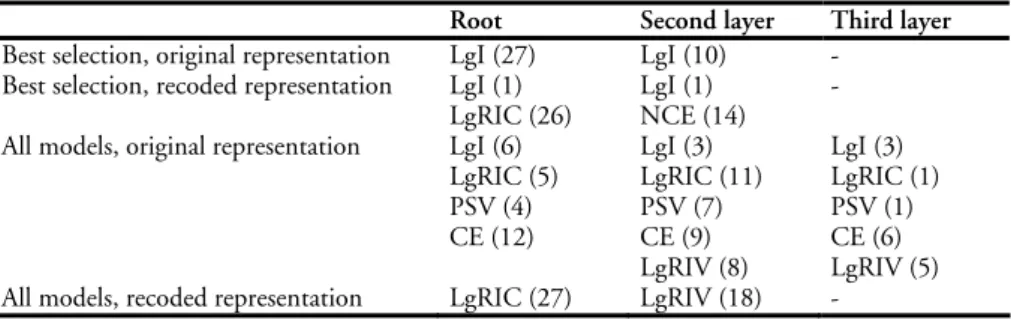
Root Second layer Third layer
Best selection, original representation LgI (27) LgI (10) - Best selection, recoded representation LgI (1)
LgRIC (26)
LgI (1) NCE (14)
-
All models, original representation LgI (6) LgRIC (5) PSV (4) CE (12)
LgI (3) LgRIC (11) PSV (7) CE (9) LgRIV (8)
LgI (3) LgRIC (1) PSV (1) CE (6) LgRIV (5) All models, recoded representation LgRIC (27) LgRIV (18) -
Table 6. Summary of important split variables in the trees
The values in parenthesis are the number of trees where the characteristic was used to split a node. LgRIC, LgI and to some extent also CE/NCE are the most important variables in the trees. Much fewer of the characteristics were needed to predict the best selection. LgI, measuring the number of instances, was more important for the original representation. For the recoded representation, the LgRIC, measuring the ratio of instances to classes, was more important. Obviously, the hardest problem was to predict the original representation with all models. This is also visible in the variety of split characteristics used for this problem.
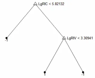
Figure 4. Example of a decision tree for the recoded representation trained on all models.
The interpretation of the decision tree is that data sets, where the ratio between instances and classes is high and the ratio between instances and variables is low, are classified as suitable for rule extraction. Loosely put, rule extraction is, according to this study, more likely to succeed for data sets with many instances and input variables but few classes.
Conclusions
The task to predict whether or not a data set is suitable for rule extraction was found to be more dependent on the representation than was expected before this study. The accuracy on the recoded representation is rather good, especially when all models are considered.
The overall conclusion must be that it is possible to predict whether or not a data set is suitable for rule extraction, if the problem is represented in a favorable way. This, together with the fact that for many data sets the combination of a high accuracy technique followed by rule extraction outperforms techniques like decision trees on accuracy, makes the proposed setup interesting.
that when the accuracy improves on the opaque model it is also easier to get good extracted models.
The criteria that are important are LgRIC, LgI and CE/NCE. This means that the number of classes (and to some extent also the distri-bution of instances among the classes) together with the number of instances are the most important criteria.
Discussion
First of all, there is a need for a second study where a specialized rule extraction algorithm is used instead of CART. We believe, based on pre-vious work, that the outcome might be slightly different. More specifically, we think that in such study a higher percentage of all opaque models will be found “suitable for rule extraction”. Clearly, this only reinforces the potential of the proposed setup and the importance of being able to predict the outcome of applying rule extraction.
It is also necessary to systematically evaluate different representation schemes that will make it easier to predict the suitability of rule extrac-tion.
Obviously the result of this study is just a small step in the direction of a more automated data mining process. Nevertheless, we think that this is a route that must be pursued. Data mining, as used by business, is currently too much art and too little science. Many vital decisions, such as choice of technique, have to be made early in the process, often based on conflicting facts and without sufficient support. We think that data mining tools must help the data miner with decisions like this and should ultimately include features like wizards or even automated choices.
suggest a fully automated choice of technique, applicable to many data mining situations.
Tuve Löfström is a fresh Ph.D. student at the Department of Business and Informatics, University College of Borås. He holds an M.Sc. in Informatics from the University College of Borås. His research interests include data mining, meta learning and soft computing.
E-mail: [email protected]
Ulf Johansson is a lecturer in informatics at the Department of Business and Informatics at the University College of Borås. He holds an M.Sc. in Computer Science and Computer Engineering from Chalmers University of Technology, and a Lic.Tech. from the Institute of Technology at Linköping University. Ulf Johansson is a member of the AI research group at the University of Skövde and his research interests include AI, machine learning, data mining, neural networks and evolutionary computation.
Notes
1. CRoss-Industry Standard Process for Data Mining was an ESPRIT project that started in the mid 1990’s. The purpose of the project was to propose a non-proprietary industry standard process model for data mining. For details see <http://www.crisp-dm.org>.
2. It should be noted that, strictly speaking, the terms transparency and comprehensi-bility are not synonymous. A neural network could, for instance, be regarded as transparent, i.e. the topology, activation functions and the weight matrix can easily be turned into a functional description. However, following the standard terminology, the distinction is not vital in this paper. The main point is that transparency without comprehensibility is of limited value.
3. Data can be coded in different ways when used by learning algorithms. The chosen representation might be important for the success of rule extraction. For more details see the section on Data representation.
References
berry, m.j.a. & g. linoff (1997). Data Mining Techniques: For Marketing, Sales, and Customer Support. New York: Wiley.
berry, m.j. a. & g. linoff (2000). Mastering Data Mining: The Art and Science of Customer Relationship Management. New York: Wiley.
blake, c.l. & c.j. merz (1998). UCI Repository of Machine Learning Databases. Irvine, CA: Department of Information and Computer Science, University of California. <http://www.ics.uci.edu/~mlearn/MLRepository.html> [2005-03-11]
breiman, l. et al. (1984). Classification and Regression Trees. Belmont, CA: Wadsworth.
brodley, c. (1994). Recursive Automatic Algorithm Selection for Inductive Learning. Diss. University of Massachusetts.
craven, m. (1996). Extracting Comprehensible Models from Trained Neural Networks. Diss. Madison: University of Wisconsin.
craven, m. & j. shavlik (1995). “Investigating the Value of a Good Input Representation.” Computational Learning Theory and Natural Learning Systems. Vol. 3, Selecting Good Models. Cambridge, MA: MIT. 307-322.
craven, m. & j. shavlik (1997). “Using Neural Networks for Data Mining.” Future Generation Computer Systems: Special Issue on Data Mining 13.2-3: 211-229.
the crisp-dm consortium (2000). CRISP-DM 1.0. <http://www.crisp-dm.org> [2005-03-11]
dorado, j. et al. (2002). “Automatic Recurrent and Feed-Forward ANN Rule and Expression Extraction with Genetic Programming.” Proceedings of the 7th
freund, y. & r.e. schapire (1996). “Experiments with a New Boosting Algorithm.” Proceedings of the 13th
Internatinal Conference om Machine Learning. Bari: Morgan Kaufmann. 148-156.
gama, j. & p. brazdil (1995). “Characterization of Classification Algorithms.” Progress in Artificial Intelligence. 7th
Portugese Conference on Artificial Intelligence (EPIA ’95; Lecture Notes in Artificial Intelligence, 990). Eds. C. Pinto-Ferreira & N.J. Mamede. Berlin: Springer. 83-102.
haykin, s. (1999). Neural Networks: A Comprehensible Foundation. 2nd ed. Upper Sadle River, NJ: Prentice Hall.
jain, a.k. & r.c. dubes (1988). Algorithms for Clustering Data. Englewood Cliffs, NJ: Prentice Hall.
johansson, u. (2004). Rule Extraction: The Key to Accurate and Comprehensible Data Mining Models. Lic. thesis. University of Linköping.
johansson, u., r. könig & l. niklasson (2003). “Rule Extraction from Trained Neural Networks using Genetic Programming.” Joint 13th
International Conference on Artificial Neural Networks and 10th
International Confernce on Neural Information Processing, ICANN/ICONIP 2003, 26-29 June 2003, Istanbul, Turkey. Supplementary Proceedings. Istanbul.13-16.
johansson, u., r. könig & l. niklasson (2004). “The Truth is in There: Rule Extraction from Opaque Models Using Genetic Programming.” 17th
Florida Artificial Intelligence Research Symposium (FLAIRS) 04. Miami, FL: AAAI Press. 658-662.
kalousis, a., j. gama & m. hilario (2004). “On Data and Algorithms: Understanding Inductive Performance.” Machine Learning 54: 275-312.
kennedy, r.l. et al. (1998). Solving Data Mining Problems Through Pattern Recognition. Englewood Cliffs, NJ: Prentice Hall.
lim, t.-s., w.-y. loh & y.-s. shih (2000). “A Comparison of Prediction Accuracy, Complexity, and Training Time of Thirty-Three Old and New Classification Algorithms.” Machine Learning 40: 203-228.
lu, h., r. setino & h. liu (1995). “Neurorule: A Connectionist Approach to Data Mining.” Proceedings of the 21st
löfström, t. & p. odqvist (2004). Rule Extraction in Data Mining: From a Meta Learning Perspective. M.Sc. Thesis. Borås: University College of Borås.
michie, d., d. spiegelhalter & c. taylor (1994). Machine Learning, Neural and Statistical Classification. (Ellis Horwood Series in Artificial Intelligence). New York: Ellis Horwood.
roiger, r.j. & m.w. geatz (2003). Data Mining: A Tutorial-Based Primer. Boston: Addison Wesley.
schapire, r.e. (1990). “The Strength of Weak Learnability.” Machine Learning 5: 197-227.