R&D expenditures by field of science and GDP: Which causes which in Canada?

(1)

Oviedo University Press 31 Economics and Business Letters

8(1), 31-40, 2019

R&D expenditures by field of science and GDP:

Which causes which in Canada?

B. Veli Doyar*

Institute of Social Sciences, Süleyman Demirel University, Isparta, Turkey

Received: 5 July 2018

Revised: 17 December 2018

Accepted: 9 January 2019

Abstract

This paper attempts to reveal the relationship between GDP per capita and R&D expenditure per capita, R&D expenditure per capita on natural sciences and engineering, and R&D expenditure per capita on social sciences and humanities for Canada. Based on data from 1981 to 2014, bootstrap causality test proposed by Hacker and Hatemi-J (2006) show that there is a unidirectional causality from GDP per capita to R&D expenditure per capita, and a unidirectional causality from GDP per capita to R&D expenditure per capita on natural sciences and engineering. However, no causal relationship is observed between R&D expenditure per capita on social sciences and humanities and GDP per capita. These results may point an indirect relationship between the variables or the validity of R&D paradox and the European paradox for Canada.

Keywords: R&D; GDP; economic growth; causality; Canada JEL Classification Codes: C32, O30, O32, O40

1. Introduction

Research and development (R&D) is accepted as one of the key drivers of economic growth today. Economic growth is an indicator of a country’s welfare, and it indicates (generally yearly) percentage change in a country’s real gross domestic product (GDP). Many countries focus on R&D policies since one of the crucial goals of a country is economic growth. In the simplest form, R&D activities enable knowledge production, innovation, productivity, and technological progress which will bring economic growth. Therefore, there exists a substantial linkage be-tween R&D activities and economic growth.

*_{E-mail: bvdoyar@gmail.com.}

Citation: Doyar, B. V. (2019) R&D expenditures by field of science and GDP: Which causes which in Canada?,

(2)

Economic growth models proposed by Solow (1956) and Swan (1956) are known as

Neo-classical growth theories. They show that how technological progress provides economic growth in an economy. The part of output growth which cannot be explained by labor and cap-ital has entered the literature as ‘Solow residual’, and attributed to technology. However, these Neo-Classical growth theoreticians assume technology as an exogenous variable. In other words, technology is believed to be constant. After a while, unlike Solow and Swan, the econ-omists who form endogenous growth models explain the technological progress in detail. The word ‘endogenous’ comes from the fact that technology is included in models as an endogenous variable. These models base technological progress upon some economic variables, and show that how growth is provided. A well-known endogenous growth theory is proposed by Arrow (1962). He defines learning as a product of experience, and suggests an endogenous growth theory that explains shifts in production function through changes in knowledge. Accordingly, knowledge production increases thanks to learning-by-doing, and the economy grows. Lucas (1988) emphasizes the prominence of human capital on growth through schooling as well as learning-by-doing. Lastly, Romer (1990) highlights R&D activities. In his model, R&D is con-sidered as a separate sector, and advances in this sector (i.e. new products developed) provide economic growth.

R&D intensity (R&D expenditures/GDP) is an important indicator in terms of a country’s economic performance. First, we look at country groups. According to data from OECD’s (2018) statistics website, the intensity is 2.35% for OECD countries, and 1.94% for European Union countries in 2016. In 2015, the intensity for the whole world was recorded as 2.2% (World Bank, 2018). When we look at the top countries in the R&D intensity, we see that the intensity was 4.25% in Israel, 4.24% in Korea, and 3.25% in Sweden. For Canada, this indicator is 1.6% in 2016, and under the country group averages mentioned above (OECD, 2018).

Using various elasticity estimation techniques, most of the studies in the literature show that innovative activities have positive effects on output or productivity. For example, Hanel (2000) for Canada; Wakelin (2001) for the United Kingdom; Sylwester (2001) for G7 countries; Wang and Tsai (2004) for Taiwan; and Ülkü (2004) for OECD countries find positive relationship between innovation activities and output or productivity.

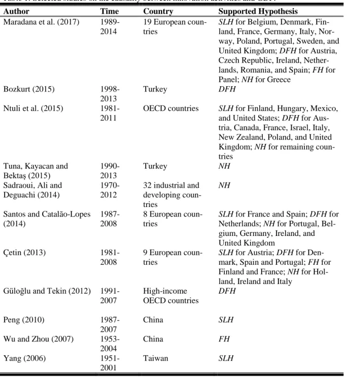
In the literature on causality, four hypotheses are classified by Maradana et al. (2017) by the way of causality between innovation activities and GDP. These are demand-following esis, supply-leading hypothesis, feedback hypothesis, and neutrality hypothesis. These hypoth-eses can be explained simultaneously with the literature which is summarized in Table 1. De-mand-following hypothesis (DFH) is supported when GDP causes innovation activities (see Maradana et al., 2017; Bozkurt, 2015; Ntuli et al., 2015; Santos and Catalão-Lopes, 2014; Çetin, 2013; and Güloğlu and Tekin, 2012). Supply-leading hypothesis (SLH) is supported when in-novation activities cause GDP (see Maradana et al., 2017; Ntuli et al., 2015; Çetin, 2013; Santos and Catalão-Lopes, 2014; Peng, 2010; and Yang, 2006). Feedback hypothesis (FH) reflects two-way causality between innovation activities and GDP (see Maradana et al., 2017; Çetin, 2013; and Wu and Zhou, 2006). Finally, neutrality hypothesis (NH) indicates the absence of causality between innovation activities and GDP (see Maradana et al., 2017; Ntuli et al., 2015; Tuna, Kayacan and Bektaş, 2015; Sadraoui, Ali and Deguachi, 2014; Santos and Catalão-Lopes, 2014; and Çetin, 2013). As seen on Table 1, the only available causality work for Canada is Ntuli et al. (2015). Among other results, they find GDP causes research output in Canada, which sup-ports DFH.

(3)

sciences and engineering. But, no causality is observed between R&D expenditure per capita

on social sciences and humanities and GDP per capita.

In the rest of the paper, second part explains data, models and methodology, third part gives empirical results, and the last part concludes.

Table 1. Selected studies on the causality between innovation activities and GDP.

Author Time Country Supported Hypothesis

Maradana et al. (2017)

1989-2014

19 European coun-tries

SLH for Belgium, Denmark,

Fin-land, France, Germany, Italy, Nor-way, Poland, Portugal, Sweden, and

United Kingdom; DFH for Austria,

Czech Republic, Ireland,

Nether-lands, Romania, and Spain; FH for

Panel; NH for Greece

Bozkurt (2015)

1998-2013

Turkey DFH

Ntuli et al. (2015)

1981-2011

OECD countries SLH for Finland, Hungary, Mexico,

and United States; DFH for

Aus-tria, Canada, France, Israel, Italy, New Zealand, Poland, and United

Kingdom; NH for remaining

coun-tries Tuna, Kayacan and

Bektaş (2015)

1990-2013

Turkey NH

Sadraoui, Ali and Deguachi (2014)

1970-2012

32 industrial and developing coun-tries

NH

Santos and Catalão-Lopes (2014)

1987-2008

SLH for France and Spain; DFH for

Netherlands; NH for Portugal,

Bel-gium, Germany, Ireland, and United Kingdom

Çetin (2013)

1981-2008

SLH for Austria; DFH for

Den-mark, Spain and Portugal; FH for

Finland and France; NH for

Hol-land, Ireland and Italy Güloğlu and Tekin (2012)

1991-2007

High-income OECD countries

DFH

Peng (2010)

1987-2007

China SLH

Wu and Zhou (2007)

1953-2004

China FH

Yang (2006)

1951-2001

Taiwan SLH

2. Data, models and methodology

2.1. Data

(4)

on natural sciences and engineering, gross domestic R&D expenditure on social sciences and

humanities, and gross domestic R&D expenditure on all fields of science. These series are mul-tiplied by 1 million to get rid of ‘millions’ notation and also divided by total population series acquired from World Bank’s (2018) World Development Indicators to get per capita values.

Figure 1 displays the timeline of the R&D series used in this study. As seen, R&D expenditure per capita on social sciences and humanities are substantially lower than R&D expenditure per capita on natural sciences and engineering. Until 2001, R&D expenditure per capita on natural sciences and engineering has increased considerably. However, R&D expenditure per capita on social sciences and humanities follows almost a straight path.

Figure 1. R&D expenditures in Canada (per capita, constant 2010 prices, PPPs, US$).

2.2. Models and methodology

Following the literature, GDP per capita is simply described as functions of R&D expenditures per capita. All variables are used in their natural logarithms, and abbreviated as ln 𝐺𝐷𝑃 for GDP per capita; ln 𝑅𝐷 for R&D expenditure per capita; ln 𝑅𝐷𝑁 for R&D expenditure per capita on natural sciences and engineering; and ln 𝑅𝐷𝑆 for R&D expenditure per capita on social sciences and humanities. Models used in causality analyses can be indicated in vector autoregression (VAR) form with lag augmentations as follows:

Model (A) - 𝐴_𝑡 = 𝛽₀+ 𝛽₁𝐴_𝑡−1+ ⋯ + 𝛽_𝑝_𝑎𝐴_𝑡−𝑝_𝑎+ ⋯ + 𝛽_𝑝_𝑎_+𝑑_𝑎𝐴_𝑡−𝑝_𝑎_−𝑑_𝑎+ 𝜀_𝑡 (1)

Model (B) - 𝐵_𝑡= 𝜃₀+ 𝜃₁𝐵_𝑡−1+ ⋯ + 𝜃_𝑝_𝑏𝐵_𝑡−𝑝_𝑏+ ⋯ + 𝜃_𝑝_𝑏_+𝑑_𝑏𝐵_𝑡−𝑝_𝑏_−𝑑_𝑏+ 𝜖_𝑡 (2)

Model (C) - 𝐶_𝑡= 𝛾₀+ 𝛾₁𝐶_𝑡−1+ ⋯ + 𝛾_𝑝_𝑐𝐴_𝑡−𝑝_𝑐+ ⋯ + 𝛾_𝑝_𝑐_+𝑑_𝑐𝛾_𝑡−𝑝_𝑐_−𝑑_𝑐+ 𝑒_𝑡 (3)

Here, 𝐴_𝑡, 𝐵_𝑡, and 𝐶_𝑡 are 2 × 1ln 𝐺𝐷𝑃 and ln 𝑅𝐷; ln 𝐺𝐷𝑃 and ln 𝑅𝐷𝑁; and ln 𝐺𝐷𝑃 and ln 𝑅𝐷𝑆

vectors, respectively. Also, 𝛽₀, 𝜃₀ and 𝛾₀ are 2 × 1 constant term vectors, and 𝛽_𝑟, 𝜃_𝑟, and 𝛾_𝑟 are

2 × 2 coefficient matrices for lag 𝑟 = 1, 2, … , 𝑝. Finally, 𝜀𝑡, 𝜖𝑡, and 𝑒𝑡 are 2 × 1 error vectors. Note that 𝑝 is optimum lag length for associated VAR model, and to be determined using Hatemi-J Criterion (HJC) (Hatemi-J 2003, 2008; Hacker and Hatemi-J, 2008), which combines Schwarz (1978) and Hannan and Quinn (1979) criteria, and gives one optimum lag length. 𝑑 is maximum integration order of the series, to be detected by unit root tests Augmented Dickey-Fuller (1981) (ADF) and Phillips-Perron (1988) (PP), in the related VAR model. Sub-indices of

0 100 200 300 400 500 600 700 800 1 9 8 1 1 9 8 3 1 9 8 5 1 9 8 7 1 9 8 9 1 9 9 1 1 9 9 3 1 9 9 5 1 9 9 7 1 9 9 9 2 0 0 1 2 0 0 3 2 0 0 5 2 0 0 7 2 0 0 9 2 0 1 1 2 0 1 3 R&D expenditures

R&D expenditures on natural sciences and engineering

(5)

𝑝 and 𝑑 indicate the models in which 𝑝 and 𝑑 belong to.

The test proposed by Granger (1969) is commonly used in investigating causation between the variables interested. However, the test results may lead to void implication, if the series are not stationary (Granger and Newbold, 1974). Also, causality between integrated variables in their levels cannot be tested using VAR models, since asymptotic distribution theory is not valid, as Sims, Stock and Watson (1990) point. Toda and Yamamoto (1995) indicate the estima-tion of VAR models that are formulated in their levels, and testing general constraints in param-eter matrices, tough the processes are integrated or cointegrated at random levels. The null hy-pothesis of “𝑘’th element of 𝐴_𝑡 does not Granger-cause 𝑗’th element of 𝐴_𝑡” can be checked through modified Wald statistic (MWALD), as Toda and Yamamoto (1995) indicate. Employing Monte Carlo simulations, however, Hacker and Hatemi-J (2006) clarify that if the sample is small, and error terms are autoregressive conditional heteroskedastic (ARCH) and non-normal, then MWALD may give invalid results. To solve this problem, they make use of bootstrap cor-rection technique, and get credible critical values. For bootstrapping, Model (A) is estimated with null of no causality first. Thereafter, bootstrapped data 𝐴𝑡∗ are generated based on estimated coefficients (𝛽̂₀, 𝛽̂₁, … , 𝛽̂_𝑝_𝑎), the essential data (𝐴_𝑡−1, … , 𝐴_𝑡−𝑝_𝑎), and bootstrapped residuals (𝜀̂_𝑡∗_{). Bootstrapped residuals are contingent upon}_𝑇_{arbitrary draws with replacement from the} regression’s modified residuals. Every single draw has probability equals to 1/𝑇, where 𝑇 is sample size. To make the expected value of the bootstrapped residuals exactly zero, the mean of the resulting set of drawn modified residuals is subtracted from every modified residual in that set. Using leverages, modified residuals, which are the unadjusted residuals of the regres-sion that are set to have constant variance, are obtained. Bootstrap simulation is performed 1000 times and MWALD statistic is estimated in every stage. Then the 𝛼’th upper quantile of the distribution of bootstrapped MWALD statistic is found and the 𝛼-level bootstrap critical values (𝑐_𝛼∗_{) are obtained. If MWALD is greater than}_𝑐

𝛼∗, then the null is rejected. The same procedure is also valid for Model (B) and Model (C).

Unit root tests and diagnostic checks on stability, serial correlation, and normality were run on Eviews 10. Leveraged bootstrap simulations, HJC, and autoregressive conditional heteroske-dasticity LaGrange multiplier (ARCH LM) test by Hacker and Hatemi-J (2005) were applied on GAUSS Light 9 by running modules of Hacker and Hatemi-J (2009a), (2009b), and (2009c), respectively.

3. Empirical results

Outcomes of ADF and PP unit root tests presented in Table 2 support that the variables are stationary in their first differences. Therefore, augmentation lags (𝑑) are set 1 for all models. When we set the maximum lag order to 3, HJC suggests optimal lag orders 2 for Model (A) and Model (B), and 1 for Model (C). VAR estimations of all models pass stability, serial correlation, and ARCH LM tests. However, when Model (A) and Model (B) pass normality test, Model (C) fails (see Tables A1, A2, A3, and A4 in Appendices).

Table 2. Results of unit root tests.

ADF (Constant) ADF (Trend) PP (Constant) PP (Trend)

Level 1st_Dif. _Level ₁st_Dif. _Level ₁st_Dif. _Level ₁st_Dif.

ln 𝐺𝐷𝑃 -1.5596 -4.5433*** _-2.6576 _-4.5598*** _-0.5090 _-4.5433*** _-2.0731 _-4.5777***

ln 𝑅𝐷 -1.6440 -3.0894** _-0.1269 _-3.5997** _-2.1647 _-3.0595** _0.3701 _-3.5346*

ln 𝑅𝐷𝑁 -1.7942 -3.2036** _0.1254 _-4.1002** _-2.3593 _-3.1544** _0.6300 _-3.7832**

ln 𝑅𝐷𝑆 0.2293 -4.2285*** _-2.1190 _-4.3265*** _0.0446 _-4.2285*** _-1.5683 _-4.3497***

(6)

Now three reasons can be put forward on the selection of bootstrap causality procedure

pro-posed by Hacker and Hatemi-J (2006). First, having a small sample with 34 observations. Sec-ond, having non-stationary series. Third, non-normal distributed residuals of Model (C).

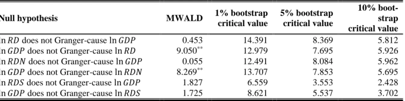
Table 3. Results of bootstrap causality tests.

Null hypothesis MWALD 1% bootstrap

critical value

5% bootstrap critical value

10% boot-strap critical value

ln 𝑅𝐷 does not Granger-cause ln 𝐺𝐷𝑃 0.453 14.391 8.369 5.812

ln 𝐺𝐷𝑃 does not Granger-cause ln 𝑅𝐷 9.050** _12.979 _7.695 _5.926

ln 𝑅𝐷𝑁 does not Granger-cause ln 𝐺𝐷𝑃 0.055 12.491 8.084 5.962

ln 𝐺𝐷𝑃 does not Granger-cause ln 𝑅𝐷𝑁 8.269** _13.707 _7.853 _5.695

ln 𝑅𝐷𝑆 does not Granger-cause ln 𝐺𝐷𝑃 1.827 6.559 3.553 2.428

ln 𝐺𝐷𝑃 does not Granger-cause ln 𝑅𝐷𝑆 1.725 8.621 5.537 3.702

Note: **_{represents the rejection of the null at 5% significance level.}

According to the results given in Table 3, null hypotheses of ‘ln 𝐺𝐷𝑃 does not Granger-cause

ln 𝑅𝐷’ and ‘ln 𝐺𝐷𝑃 does not Granger-cause ln 𝑅𝐷𝑁’ are both rejected at 5% significance level. Consequently, there is a unidirectional causality from GDP per capita to R&D expenditure per capita, and a unidirectional causality from GDP per capita to R&D expenditure per capita on natural sciences and engineering in Canada.

4. Conclusions

In this study, the relationship between per capita GDP and R&D expenditures per capita by field of science are examined for Canada over the period from 1981 to 2014. Having a small sample, non-stationary series and non-normal distributed error terms are the reason why bootstrap cau-sality test proposed by Hacker and Hatemi-J (2006) is chosen. The first finding points to a unidirectional causality from GDP per capita to R&D expenditure per capita. This result is compatible with the results of Maradana et al. (2017); Bozkurt (2015); Çetin (2013); and Gü-loğlu and Tekin (2012). It is particularly in harmony with Ntuli et al. (2015) whose results show causality from GDP to research output for Canada. Also, a unidirectional causality from GDP per capita to R&D expenditure per capita on natural sciences and engineering is found. How-ever, no causal relationship is observed between R&D expenditure per capita on social sciences and humanities and GDP per capita.

As seen, no evidence that supports ‘supply-leading hypothesis’ is found for Canada. In other words, R&D expenditures does not cause economic growth. In point of R&D expenditure per capita and R&D expenditure per capita on natural sciences and engineering, the results clearly show R&D expenditures originate from economic growth. These findings indicate the validity of ‘demand-following hypothesis’ in Canada. In this regard, the country can stimulate innova-tion activities as the economy grows.

In terms of social sciences, ‘neutrality hypothesis’ is supported for Canada. Thus, R&D ex-penditures on social sciences and humanities and GDP have no effect on each other. As shown in data subsection, Canada spends far less money on R&D in social sciences and humanities than in natural sciences and engineering. This can limit both quantity and quality of social stud-ies, and be the reason why the causal link is broken. This field deals with humans, who are also economic agents that constitute the economy, by its very nature. Thus, R&D expenditures on social sciences can be related to economic growth through social channels. That is to say, there can be an indirect relationship.

(7)

Swedish version of R&D paradox indicates high R&D expenditure but comparatively low GDP

(Ejermo, Kander, and Henning, 2011). Likewise, European paradox indicates high performance in science and low performance in high-tech sectors (European Commission, 1995).

Figure 2. GDP per capita and R&D expenditures per capita by field of science, index 1981=1.

Ejermo, Kander, and Henning (2011) investigate the timeline of value added and R&D ex-penditures by sector. They explain the growing gap between value added and R&D exex-penditures in fast-growing manufacturing and service sectors in Sweden as R&D paradox. Following Ejermo, Kander, and Henning (2011), same procedure is applied using variables employed in empirical analysis. The variables are indexed (1981=1) to get a clean comparison. The timeline is given on Figure 2. Index forms of GDP per capita, R&D expenditure per capita, R&D ex-penditure per capita on natural sciences and engineering, and R&D exex-penditure per capita on social sciences and humanities abbreviated as GDP index, RD index, RDN index, and RDS index, respectively. It is seen that the gap between GDP index and RD index, as well as GDP index and RDN index, typically widens in time. There is almost no gap between GDP index and RDS index in 1981-1993 when the gap is negative in 1994-1998. After 1998, the gap be-comes positive and also widens in time. These findings can be due to R&D and European par-adoxes.

Finally, further study in this area is required. Then, future research can examine the existence of the possible indirect causality between R&D expenditures and economic growth. Also, va-lidity of R&D and European paradoxes for Canada can be investigated in detail.

Acknowledgements

I would like to thank Dilek Çetin, R. Scott Hacker, and three anonymous referees for their valuable comments and suggestions.

References

Arrow, K. J. (1962) The Economic Implications of Learning by Doing, The Review of Economic Studies, 29(3), 155-173.

0.5 1 1.5 2 2.5 3 1 9 8 1 1 9 8 3 1 9 8 5 1 9 8 7 1 9 8 9 1 9 9 1 1 9 9 3 1 9 9 5 1 9 9 7 1 9 9 9 2 0 0 1 2 0 0 3 2 0 0 5 2 0 0 7 2 0 0 9 2 0 1 1 2 0 1 3

(8)

Bozkurt, C. (2015) R&D Expenditures and Economic Growth Relationship in Turkey,

Interna-tional Journal of Economics and Financial Issues, 5(1), 188.

Çetin, M. (2013) The Hypothesis of Innovation-Based Economic Growth: A Causal Relation-ship, International Journal of Economic and Administrative Studies, (11), 1-16.

Dickey, D. A. and Fuller, W. A. (1981) Likelihood Ratio Statistics for Autoregressive Time Series with a Unit Root, Econometrica, 49(4), 1057-1072. doi: 10.2307/1912517.

Ejermo, O., Kander, A., and Henning, M. S. (2011). The R&D-growth paradox arises in fast-growing sectors, Research Policy, 40, 664-672. doi:10.1016/j.respol.2011.03.004.

European Commission (1995). Green Paper on Innovation, Office for Official Publications of the European Communities.

Granger, C. W. J. (1969) Investigating Causal Relations by Econometric Models and Cross-Spectral Methods, Econometrica, 37(3), 424-438. doi: 10.2307/1912791.

Granger, C. W., and Newbold, P. (1974) Spurious regressions in econometrics, Journal of econ-ometrics, 2(2), 111-120. doi: 10.1016/0304-4076(74)90034-7.

Güloğlu, B., and Tekin, R. B. (2012) A Panel Causality Analysis of the Relationship Among Research and Development, Innovation, and Economic Growth in High-Income OECD Countries, Eurasian Economic Review, 2(1), 32-47. doi: 10.14208/BF03353831.

Hacker, R. S. and Hatemi-J, A. (2005) A test for multivariate ARCH effects, Applied Econom-ics Letters, 12(7), 411-417. doi: 10.1080/13504850500092129.

Hacker, R. S. and Hatemi-J, A. (2006) Tests for Causality Between Integrated Variables Using Asymptotic and Bootstrap Distributions: Theory and Application, Applied Economics, 38, 1489-1500. doi: 10.1080/00036840500405763.

Hacker, R. S. and Hatemi-J, A. (2008) Optimal Lag Length Choice in the Stable and Unstable VAR Models under Situations of Homoscedasticity and ARCH, Journal of Applied Statis-tics, 35(6), 601-615. doi: 10.1080/02664760801920473.

Hacker, R. S. and Hatemi-J, A. (2009a) HHtest: GAUSS Module to Implement Bootstrap Test for Causality with Leverage Adjustments, Statistical Software Components G00005, Boston College Department of Economics.

Hacker, R. S. and Hatemi-J, A. (2009b) LagOrder: GAUSS module to determine the optimal lag order in the VAR model based on Information Criteria, Statistical Software Components G00008, Boston College Department of Economics.

Hacker, R. S. and Hatemi-J, A. (2009c) MV-ARCH: GAUSS module to implement the multi-variate ARCH test, Statistical Software Components G00009, Boston College Department of Economics.

Hanel, P. (2000) R&D, Interindustry and International Technology Spillovers and The Total Factor Productivity Growth of Manufacturing Industries in Canada, 1974-1989, Economic Systems Research, 12(3), 345-361. doi: 10.1080/09535310050120925.

Hannan, E. J. and Quinn, B. G. (1979) The determination of the order of an autoregres-sion, Journal of the Royal Statistical Society. Series B (Methodological), 190-195.

Hatemi-J, A. (2003) A New Method to Choose Optimal Lag Order in Stable and Unstable VAR Models, Applied Economics Letters, 10(3), 135-137. doi: 10.1080/1350485022000041050. Hatemi-J, A. (2008) Forecasting Properties of a New Method to Determine Optimal Lag Order

in Stable and Unstable VAR models, Applied Economics Letters, 15(4), 239-243. doi: 10.1080/13504850500461613.

Lucas Jr, R. E. (1988) On the mechanics of economic development, Journal of monetary eco-nomics, 22(1), 3-42. doi: 10.1016/0304-3932(88)90168-7.

(9)

Ntuli, H., Inglesi-Lotz, Chang, T., and Pouris, A. (2015) Does Research Output Cause

Eco-nomic Growth or Vice Versa? Evidence from 34 OECD Countries, Journal of the Association for Information Science and Technology, 66(8), 1709-1716. doi: 10.1002/asi.23285.

OECD (2018) OECD Statistics. (accessed 25 May, 2018) http://stats.oecd.org/.

Peng, L. (2010) Study on Relationship between R&D Expenditure and Economic Growth of China, In Proceedings of the 7th International Conference on Innovation & Management, 1725-1728.

Phillips, P. C. B. and Perron, P. (1988) Testing for a Unit Root in Time Series Regression, Biometrika, 75(2), 335-346. doi: 10.2307/2336182.

Romer, P. M. (1990) Endogenous Technological Change, Journal of Political Economy, 98(5, Part 2), 71-102. doi: 10.1086/261725.

Sadraoui, T., Ali, T. B., and Deguachi, B. (2014) Economic Growth and International R&D Cooperation: A Panel Granger Causality Analysis, International Journal of Econometrics and Financial Management, 2(1), 7-21. doi: 10.12691/ijefm-2-1-2.

Santos, J. F. and Catalão-Lopes, M. (2014) Does R&D Matter for Economic Growth or Vice-Versa? An Application on Portugal and Other European Countries, Archives of Business Re-search, 2(3), 1-17. doi: 10.14738/abr.23.194.

Schwarz, G. (1978) Estimating the Dimension of a Model, The Annals of Statistics, 6(2), 461-464.

Sims, C.A., Stock, J. H. and Watson, M. W. (1990) Inference in Linear Time Series Models with Some Unit Roots, Econometrica, 58(1), 113-144. doi: 10.2307/2938337.

Solow, R. M. (1956) A Contribution to The Theory of Economic Growth, The quarterly journal of economics, 70(1), 65-94. doi: 10.2307/1884513.

Swan, T. W. (1956) Economic Growth and Capital Accumulation, Economic Record, 32(2), 334-361. doi: 10.1111/j.1475-4932.1956.tb00434.x.

Sylwester, K. (2001) R&D and economic growth, Knowledge, Technology & Policy, 13(4), 71-84. doi: 10.1007/BF02693991.

Toda, H.Y. and Yamamoto, Y. (1995) Statistical Inference in Vector Autoregressions with Pos-sibly Integrated Processes, Journal of Econometrics, 66, 225-250. doi: 10.1016/0304-4076(94)01616-8.

Tuna, K., Kayacan, E. and Bektaş, H. (2015) The Relationship Between Research & Develop-ment Expenditures and Economic Growth: The case of Turkey, Procedia-Social and Behav-ioral Sciences, 195, 501-507. doi: 10.1016/j.sbspro.2015.06.255.

Ülkü, H. (2004) R&D, innovation, and Economic Growth: An Empirical Analysis (No. 4-185). International Monetary Fund.

Wakelin, K. (2001) Productivity Growth and R&D Expenditure in UK Manufacturing Firms, Research Policy, 30(7), 1079-1090. doi: 10.1016/S0048-7333(00)00136-0.

Wang, J. C., and Tsai, K. H. (2004) Productivity Growth and R&D Expenditure in Taiwan's Manufacturing Firms, In Growth and Productivity in East Asia, NBER-East Asia Seminar on Economics, 13, 277-296.

World Bank (2018) World Development Indicators. Available via http://data-bank.worldbank.org (accessed 25 May, 2018).

Wu, Y., Zhou, L. and Li, J. X. (2007) Cointegration and Causality Between R&D Expenditure and Economic Growth in China: 1953-2004, In International Conference on Public Admin-istration, 76.

(10)

Appendix A – Additional tables

Table A1. Roots of characteristic polynomial.

Model (A) Model (B) Model (C)

Root Modulus Root Modulus Root Modulus

0.979034- 0.089139i 0.983083 0.985065-0.083223i 0.988574 0.982276 0.982276 0.979034+0.089139i 0.983083 0.985065+0.083223i 0.988574 0.837936 0.837936

0.241528-0.264432i 0.358135 0.219617-0.271096i 0.348891 0.241528+0.264432i 0.358135 0.219617+0.271096i 0.348891

Table A2. VAR residual serial correlation LM tests.

Lags LRE-Stat* Prob LRE-Stat* Prob LRE-Stat* Prob

1 7.4512 0.1139 6.3732 0.1730 5.7718 0.2169

2 3.2891 0.5107 4.0887 0.3941 2.7459 0.6012

3 3.7636 0.4389 3.4711 0.4823 1.4408 0.8371