Research Report No. ROSE-2005/02
Dynamic Behaviour of Reinforced Concrete Frames Designed
with Direct Displacement-Based Design
by
J. Didier Pettinga
Graduate Student
M.J. Nigel Priestley
Co-Director
ROSE School c/o EUCENTRE Via Ferrata 1, 27100, Pavia, Italy
1. INTRODUCTION ... 1
1.1 OBJECTIVES AND INTENT... 2
2. CURRENT DESIGN APPROACHES... 5
2.1 INTRODUCTION... 5
2.2 FORCE-BASE DESIGN METHODS ... 5
2.2.1 Equivalent Static Lateral Force Method ... 6
2.2.2 Multi-modal Superposition...10
3. DISPLACEMENT-BASED DESIGN METHOD...15
3.1 DIRECT DISPLACEMENT-BASED DESIGN ...15
3.1.1 Introduction...15
3.1.1 Direct Displacement-Based Design Method ...16
4. DDBD FRAME DESIGN PROCEDURES...23
4.1 GENERALISED DESIGN PROCEDURE...23
4.2 DESIGN PROCEDURE AS APPLIED TO THIS STUDY ...25
4.2.1 Frame Descriptions ...25
4.2.2 Displacement Design Spectrum...26
4.2.3 Direct Displacement-based Design Parameters ...30
4.2.4 Section Analysis ...33
5. INELASTIC TIME-HISTORY ANALYSES...41
5.1 MODELLING ASSUMPTIONS...41
5.2 SPECIFIC MODEL DETAILS AND DEFINITIONS ...42
5.2.1 Model type and geometry ...42
5.2.2 Member bilinear factors and plastic hinge properties...44
5.2.3 Modified Takeda Hysteresis rule ...44
5.2.4 Viscous damping...45
5.2.5 P-∆ Effects ...46
5.2.6 Input ground motions...46
6. INITIAL INELASTIC TIME-HISTORY RESULTS...49
6.1 MAXIMUM DRIFT AND DISPLACEMENT PROFILES ...49
6.2.1 Design displacement profile developments... 51
6.2.2 Distribution of beam strengths ... 57
6.2.3 Dynamic amplification of storey drifts... 61
6.3 SUMMARY OF PROPOSED CHANGES TO THE DIRECT DISPLACEMENT-BASED FRAME DESIGN PROCEDURE. ... 67
7. IMPLEMENTATION OF SUGGESTED DDBD PROCEDURES ... 69
7.1 REVISED DIRECT DISPLACEMENT-BASED DESIGNS ... 69
7.2 INELASTIC TIME-HISTORY RESULTS USING REVISED DDBD METHODS ... 78
7.2.1 Description of results... 78
7.2.2 Comments on results ... 86
8. ACCOUNTING FOR DYNAMIC AMPLIFICATION ... 95
8.1 APPLICATION OF EXISTING METHODS ... 95
8.1.1 FORCE-BASED AMPLIFICATION APPROACHES... 95
8.1.2 DDBD DYNAMIC AMPLIFICATION METHOD: MODIFIED MODAL SUPERPOSITION ... 100
8.2 DEVELOPMENT OF DYNAMIC AMPLIFICATION PROCEDURES FOR FRAME DESIGN... 101
8.2.1 Column shear force amplification... 104
8.2.2 Column bending moment amplification ... 114
8.3 VERIFICATION WITH REAL EARTHQUAKE ACCELEROGRAMS... 118
8.4 MODIFICATION FOR TWO-WAY FRAMES... 122
8.5 SUMMARY OF PROPOSED METHODS OF ACCOUNTING FOR DYNAMIC AMPLIFICATION ... 122
9. PARAMETRIC INVESTIGATION AND FURTHER DISCUSSION... 125
9.1 VARIATION OF BEAM DEPTH ... 125
9.1.1 Time-history results and application of amplification methods... 126
9.2 INCREASED BEAM SPANS... 130
9.3 DRIFT AMPLIFICATION DEPENDENCY ON INTENSITY... 131
9.4 SUMMARY OF PARAMETRIC STUDY... 134
10. CONCLUSIONS ... 137
10.2 DDBD METHODS OF ACCOUNTING FOR DYNAMIC AMPLIFICATION IN FRAMES ...139 10.3 FUTURE DEVELOPMENTS ...140 REFERENCES...143 APPENDIX A TIME HISTORY RESULTS USING 5 REAL ACCELEROGRAMS
Reinforced concrete frame structures are a common building form in seismically active regions. However, the use of such structural forms and the inherent variability in geometric proportions, sectional shapes and material properties means that the dynamic behaviour under earthquake loading has been, and remains, difficult to consistently evaluate.
Developments in seismic design of reinforced concrete structures can largely be attributed to research aimed at better understanding the mechanics of concrete behaviour and thus improving the detail design methods applied to structural and non structural elements. This has reached the extent that in some forms, code requirements are such that newly designed buildings can be considered sufficiently safe under seismic excitation.
Fundamental to the process of seismic design, has been the use of force-based design whereby a set of external forces, seen as equivalent to the inertial forces induced by ground accelerations, are applied to the structure. These design methods are often based on the key assumption that dynamically, the structure will behave principally with first mode response, with requirements for using multi-modal analysis when certain limits structural behaviour are not met. In many situations the first mode dominance is a valid assumption, however it is not necessarily satisfactory to disregard the presence of vibration modes above the fundamental, the so called ‘higher modes’.
Studies reported by Paulay (1977), and further presented by Paulay and Priestley (1992), showed that higher modes do in fact play a significant role in reinforced concrete frame and wall behaviour, and that approaches to encompass these effects must be considered, especially when using simplified analysis methods such as the equivalent static lateral force-based approach.
Current code provisions in New Zealand (NZS 4203;1992 and NZS 3101;1995) have adopted the procedures described by Paulay and Priestley (1992), thereby accounting for the presence of higher mode effects using simplified equations that act to scale-up the design moments and shears such that the design envelope should provide sufficient capacity to prevent exceedance under earthquake demands.
Recent work presented by Priestley and Amaris (2002) looked at the dynamic behaviour of reinforced concrete structural walls designed using direct displacement-based design. The results added further emphasis to the importance of dynamic amplification, and emphasises that the current code provisions are in many cases insufficient. As a result of this work a modified form of the commonly used elastic modal superposition, was put forward as a simple and generally very effective approach to accounting for dynamic amplification of wall shear forces and bending moments.
Preliminary studies on frame behaviour designed with direct displacement-based design by Priestley (2003) have however suggested that the method found for wall structures does not transfer to frames in a succinct manner. Results were generally inconsistent and often gave a poor fit to mean envelopes found from inelastic time-history analyses. Hence the need for further work to develop a rational and simple approach for frame structures.
1.1 OBJECTIVES AND INTENT
Because the equations applied in design codes for frame dynamic behaviour were developed using force-based design procedures, it is important to check these methods with displacement-based design approaches to verify if and what differences there are in the dynamic behaviour of buildings designed with such processes.
The apparent inability of the modified modal superposition approach to accurately predict the dynamic behaviour of frame structures is due to many factors. However, one particular issue is that of the variability in geometric parameters. To this extent the research results presented here, attempts to narrow the geometric bounds, such that the behaviour of one particular form of simple frame structure can be assessed. The use of relatively deep beams and short spans has been adopted in what might be termed a ‘tube-frame’ structure, where by the perimeter frames are intended to act as the principal lateral deformation resisting components. This definition has also been made to ensure reasonable ductility demands by generating relatively stiff structures with low yield displacements. Using code drift limits normal reinforced concrete 2-way frames have ductility demands of about two, hence they would not provide a rigorous investigation of ductile dynamic behaviour.
The intent of this work is to investigate some key aspects of the direct displacement-based design method, using designs for 2, 4, 8, 12, 16 and 20 storey frames. The following points define the objectives and general method.
Using design spectrum compatible accelerograms, a series of inelastic time-history analyses of varying intensity are used to help assess the demands resulting from dynamic amplification.
A systematic investigation of the design displacement profiles and their application to ensure that drift demands satisfy the specified design drift limits. This is particularly important with respect to the ability of the method to control higher mode drift effects.
An examination of the significance of higher mode contributions to column shear forces and bending moments, in particular with respect to ductility demands and earthquake intensity.
2.
CURRENT DESIGN APPROACHES
2.1 INTRODUCTION
The standard approach for seismic design of structures, specified in many design codes, involves the development of a base shear value corresponding to a given design spectrum. This design value is often derived for a reduced level of excitation on the proviso that ductile inelastic behaviour is acceptable and allowed for at section and member levels by providing adequate detailing to ensure material behaviour that accommodates the strain demands.
From the reduced design spectrum a set of lateral force vectors can be developed to represent first mode response only, as is the case for equivalent static methods, or as a series of force vectors representing a number of modes as specified in code requirements. These lateral forces are then applied to the structure as external forces and the member actions resulting, taken directly for design or statistically combined to give final design values.
Thus the underlying intent of force-based design involves the specification and attainment of a minimum strength, based on assumptions of initial stiffness, design earthquake intensity and ductile capacity of the structure, as applied through a force reduction factor. In some cases it is required to check the structural deformations, often in the form of storey drifts, against code defined limitations, to verify the deformation behaviour of the structure. This approach contrasts strongly to that of direct displacement-based design whereby structures are designed to attain a specified level of damage commensurate with a given limit state. By specifying a target displacement-based on an equivalent single degree of freedom system, it is possible to derive values of strength, stiffness and thus structural period. This method is further outlined in Chapters 3 and 4.
2.2 FORCE-BASED DESIGN METHODS
The following sections outline the methods of generating design forces described above, including code recommendations for the application of the methods.
2.2.1 Equivalent Static Lateral Force Method
This approach utilises the key assumption that the first mode dominates the structural response to the extent that a direct account of higher modes is not required. Code limitations on the use of this method generally centre around having a first mode period less than a specified maximum and maintaining the vertical and horizontal regularity of the structure.
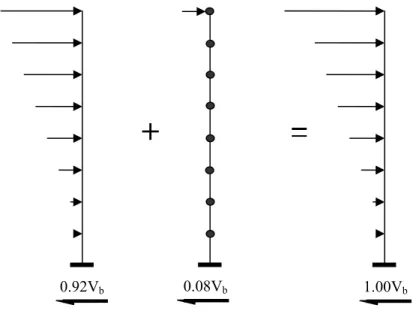
If a structure satisfies these requirements then the force vector is defined such that the distribution varies linearly up the structure as an ‘inverted triangle’. This profile thus matches the fundamental mode shape with no direct account for the higher modes. Some provision can be made, through the use of an additional proportion of force at the roof level. This extra force is specified as 8% in NZS 4203, 10 % by Paulay and Priestley (1992), and ranges from 0 to 25% for the UBC. It is noted that Eurocode 8 (EC8) does not specify this additional force.
The fundamental period of the structure can be estimated through the use of established equations such as that of the Rayleigh Method (NZS 4203:1992, EC8, UBC):
( )
(
)
∑
∑
∆ ∆ =
N i i N
i i
F g
W T
1 1
2
1 2π (2.1)
or with simple correlated approximations as suggested in EC8:
4 3 1 C H
T = t⋅ (2.2)
In which for moment resisting concrete frames up to 40m in height and H being the height in meters.
075 . 0 =
t C
Using design spectra, a value of Spectral Acceleration Sa(T1) is obtained from which the base shear can be calculated using the total seismic weight of the structure Wt.
( )
ta
b S T W
V = 1 ⋅ (2.3)
The base shear can then be distributed as an equivalent lateral force vector at each level i
(
)
∑
==
N
i i i
i i b i
h W
h W V F
1
(2.4)
This form is altered in NZS 4203 to give the additional proportion of base shear applied at the roof level, intended to account for increases in shear and moment values due to higher modes:
(
)
∑
=⋅ + =
N
i i i i i b t
i
h W
h W V F
F
1
92 . 0
(2.5)
where t b at roof level and 0 for all other levels. The lateral force distribution
resulting from this equation is seen in Figure 2-1.
V F =0.08
With this distribution of forces the global overturning and storey shear forces can be found along with individual member actions.
2.2.1.1 Methods of Dynamic Amplification.
It is clear that for taller structures this simplified approach is not adequate to account for modes above the fundamental, which tend to take greater participation as overall height increases. Thus it is foreseeable that further account could be made at a later stage of the design process. This has been used in NZS 3101 following the methods presented by Paulay and Priestley (1992) for frames and walls.
Moment Amplification: Equations are presented in NZS 3101 for both one-way and two-way frames, to account for concurrent moment capacity development in beams framing into a column, shifts in column point of contraflexure and in the case of two-way frames the reduced section efficiency for moments applied about the section diagonal axis. The amplification factor is given by ω and takes the following forms and limits for each frame type:
Figure 2-1. The concept of the Equivalent Lateral Force method with additional roof level force One-way frames1.3≤ω=0.6T1+0.85≤1.8 (2.6a)
Two-way frames1.5≤ω=0.5T1+1.1≤1.9 (2.6b) Here T1 is the fundamental period found by the methods above or some other means such as dynamic modelling with a computer program. As higher mode responses do not affect the required strength at column bases, the value of ω is taken as 1.0 for one-way frames and 1.1 for two-way frames to account for the reduced section efficiency about the diagonal section axis. These factors are also applicable at roof level where it is deemed acceptable for plastic hinges to form in the columns. With the intent of providing a gradual reduction in amplification, the minimum factor allowed in Eq.(2.6a & b) is used for the floor level immediately below the roof.
Because higher mode response is seen to be significant in the upper storeys of a structure, Eq.(2.6a & b) is applied to the upper 70% of the building. From the base to 0.3H, a linear variation in ω from 1.0 or 1.1 at the base, to the value calculated from Eq.(2.6a & b) is used.
Thus the distribution of values for the dynamic amplification factor ω can be represented schematically as in Figure 2-2.
0.92Vb 0.08Vb 1.00Vb
Figure 2-2. Schematic representation of column bending moment dynamic amplification as suggested by Paulay and Priestley (1992) for use with simplified lateral force methods
The dynamic amplification factor is applied in the design moment equation as shown:
E o
u M
M =ωφ (2.7)
where ME is the moment value from the equivalent lateral force analysis and φο is the flexural overstrength factor for plastic hinges that accounts for material overstrength and strain hardening effects. In design this factor is typically specified in relevant material design codes, such as NZS 3101 where a minimum value is defined as:
47 . 1 85 . 0
25 .
1 =
= = =
φ λ
φ o
E o o
M M
(2.8)
This value of overstrength is often higher due to practical limitations on available reinforcing bar sizes leading to excess provisions of nominal strength.
1.0 1.6 1.6 1.3
1.0 1.1
1.5 1.8
1.8
0.
3H
1.1
For the purposes of this study the flexural reduction factor is taken equal to 1.0, thus
E o
o M
M =λ , with λο calculated and removed from the time-history results following the procedure defined in Section 7.2.2.2.
Shear Amplification: It is possible to make an estimate of column shear by taking the amplified moment gradient found using the method above. It is likely that such an estimate could be excessively conservative. Therefore, with the probability of maximum amplified moments occurring simultaneously at each end of a column being sufficiently low, it is reasonable to consider another method of shear amplification.
Paulay and Priestley (1992) suggested a simple multiplicative factor that accounts for beam moment distribution into columns not following that given by an elastic analysis and thus generating a moment gradient, or shear force, larger than anticipated. This can be interpreted as a shift in the position of the point of contraflexure, and hence an account for dynamic magnification as suggested in the previous section. This approach has been adopted in NZS 3101 in the following forms:
One-way frame upper storeys Vu =1.3φoVE (2.9a)
Two-way frame upper storeys Vu =1.6φoVE (2.9b)
With typical values of φο this can result in design values of approximately 1.8VE and
2.2VE for one-way frames and two-way frames respectively.
In first storey columns where hinging is expected at the base, and should be anticipated at the top (due to inelastic first floor beam elongation), shear demands are calculated using the overstrength moments from top Mo(top)and bottom Mo(bottom)hinging:
n bottom o top o col
L M M
V = ( )+ ( ) (2.10)
where Ln is the clear height of the column from the first floor soffit to the base. Note this
should also be applied to the top storey, where it is possible that columns may form plastic hinges before the top floor beams.
2.2.2 Multi-modal Superposition
When a structure does not satisfy code requirements for any one of the following: maximum height, period, and horizontal or vertical regularity, a modal analysis and
subsequent combination is generally required (NZS 4203:1992, EC8, UBC). This procedure requires the determination of a number of vibration periods in order to include a sufficient proportion of the structural mass in the analysis. EC8 specifies this proportion to be greater than 90%, with all modes contributing greater than 5% being included (NZS 4203 is similar). Because of the consideration of the modal contributions, this method is assumed to directly account for higher mode effects, especially in the upper levels of a structure, and hence no further amplification is specified for design purposes.
Having determined these values of period and the corresponding mode shapes, the mass participation factors for each mode m can be found by the following:
∑
∑
∑
= = = ⎟ ⎟ ⎠ ⎞ ⎜ ⎜ ⎝ ⎛ = N i i N m i i im N m i i im m m m m 1 1 , 2 2 1 , 1 φ φ ρ (2.11)It is possible to obtain values of Spectral Acceleration, S (Ta ), from appropriate design
spectra. From these values the base shear corresponding to each participating mode is found by:
( )
⎟⎟ ⎠ ⎞ ⎜ ⎜ ⎝ ⎛ =∑
= N i i m m aBm S T g m
V
1
ρ (2.12)
In a similar fashion to the equivalent static lateral forces described above, the base shear for each mode is distributed as:
(
)
∑
= = N m i i im i im Bm im m m V F 1 , φ φ (2.13)These forces are applied to the structure as external loads, thus giving the modal member actions. Maximum modal displacements are found from the pseudo displacement spectrum that can be directly calculated from the design spectral accelerations by:
( )
22 4π m m a m T g T S = ∆ (2.14)This maximum displacement is used to find the modal displacement at each floor level i
by the following:
∑
∑
= = ∆ = ∆ N m i i im N m i m i im im im m m 1 , 2 1 , φ φ φ (2.15)The results obtained from the above equations are specific to each vibration mode. Under excitation such as that due to earthquake ground motion, it is unlikely that the modal maxima will occur simultaneously. Thus it is considered that a direct summation of modal quantities will produce design values that are excessively conservative. For this reason it is common to apply one of two statistical combination methods; either the Square Root Sum of the Squares (SRSS) or Complete Quadratic Combination (CQC).
The application of SRSS is limited to some extent by the requirement that two modes of vibration, i and j, are sufficiently separated in periods Ti and Tj, such that correlation
between the two modes is not significant. EC8 specifies that SRSS may be used if this separation is such that Tj ≤ 0.9Ti. The form of the SRSS combinations for equivalent
lateral forces, shears and displacements are as follows:
∑
= = N m i im i F F 1 ,2
∑
= = N m i im i V V 1 ,
2
∑
= ∆ = ∆ N m i im i 1 , 2 (2.16)
If the structure does not satisfy this constraint then a more rigorous combination that accounts for modal correlations using cross modal coefficients ρij can be used with the
following form:
∑ ∑
=
i j mi ij mj
m F F
F ρ (2.17)
Because the modal superposition method uses values of spectral acceleration, it is common to reduce the design base shear and thus applied lateral forces to allow for ductile structural response. Assuming the equal displacement approximation is valid, this reduction can simply be taken as a direct division of the elastic forces (for all the modes used) by R (the force reduction factor) or q (the behaviour factor) equal to µ∆, the design
structural displacement ductility. This value is specified in design codes for various structural forms depending on the anticipated ductile capacity of the structure. For reinforced concrete frames the value of µ∆ is usually taken between 3 and 6.
3.
DISPLACEMENT-BASED DESIGN METHOD
3.1 DIRECT DISPLACEMENT-BASED DESIGN
3.1.1 Introduction
Recent developments in seismic design philosophy have centred around the concept of performance-based design. In the past 10 years many researchers have proposed methods of design focusing on performance-based techniques (as summarised and compared by Sullivan et al., 2003). In its purest form this is an approach whereby a structure is designed, not to satisfy a set of performance requirements, but instead to meet the given criteria. In this way a structure is designed and expected to reach a specified acceptable amount of damage under one or more levels of ‘design intensity’ earthquake. Structures designed in this manner can be expected to exhibit more of a uniform risk, something that is not easily achieved using force-based procedures. It should be noted that most performance-based methods check displacements at the end of the design process, or require transverse reinforcement detailing to match calculated rotations, few procedures proposed actually design to target drift amounts.
Material strain limits are commonly used to define damage limit states. For reinforced concrete these can be defined by concrete compression strains and steel tension (or compression) strains. Often the serviceability limit state (SLS) is defined such that concrete compression strains remain lower than εc = 0.004 above which point cover spalling may occur, and corresponding steel tension strains are low enough that residual crack widths are acceptably low, for example εs = 0.010 to 0.015. In a similar fashion, a damage control limit state can be defined based on larger strain levels. For concrete compression strains this can be a function of confined concrete strains that can be estimated from allowable transverse reinforcement tension strains caused by lateral concrete expansion, such that:
(
)
'
4 . 1 004 . 0
cc suh yh s cm
f
f ε
ρ
Where ρs is the confinement volumetric ratio, fyh the transverse steel yield strength, εsuh
the transverse steel strain at maximum stress and f ’cc the confined concrete compression
strength (Mander et al. 1988).
Maximum longitudinal steel tensile strains can be set at any desired level, however for reasons relating to buckling (under reversed loading) and avoidance of low cycle fatigue (Priestley and Kowalsky, 2000) it is prudent to limit this level to the following:
su
sm ε
ε =0.6 (3.2)
Further to the specification of material strain limits, it is possible, and conceptually more straightforward, to define limit states by drift amounts. For serviceability limits this could be set at θ = 0.01 to avoid non-structural damage, while for damage-control limit states, the amount of structural damage deemed acceptable, is left to choice, however, in many cases this drift limit will be specified in design codes. For instance NZS 4203 limits inter-storey drifts to θ = 0.02 for designs completed without inelastic time-history analysis (for which θ = 0.025 is acceptable).
Underlying the displacement-based design methods is the use of displacement design spectra. Often these are a simple conversion of spectral accelerations given in design codes. Of particular importance in the definition of a displacement spectrum is the so called ‘corner-period’ beyond which peak displacements are assumed constant for increasing structural period. This reflects the fact that as structural period increases, maximum displacements tend to that of the peak ground displacement, thus for periods over a defined limit, peak displacements can be considered independent of structural period.
The following section outlines one particular form of displacement-based design, namely ‘Direct Displacement-Based Design’ (Priestley, 1993). The general method is described and appropriate equations defined, along with important assumptions underlying the design process.
3.1.1 Direct Displacement-Based Design Method
The following relations are a summary of the design process developed and described in greater detail by Priestley and Kowalsky (2000) and Priestley et. al (2004).
(c) (d) Unbonded
Prestressing
1 2 3 4 5 6
Elasto-Plastic Steel Frame Concrete Frame Da m p in g ( % ) 0 20 40 60 Displacement Ductility
0 1 2 3 4 5
0 0.1 0.2 0.3 0.4 0.5 5% 10% 15% 20% 30% ∆d Te D is p la cem en t ( m ) Period (seconds) (a) (b) FU Fn
Ki KE
rKi ∆d ∆y he me F (c) (d) Unbonded Prestressing
1 2 3 4 5 6
Elasto-Plastic Steel Frame Concrete Frame Da m p in g ( % ) 0 20 40 60 Displacement Ductility
0 1 2 3 4 5
0 0.1 0.2 0.3 0.4 0.5 5% 10% 15% 20% 30% ∆d Te D is p la cem en t ( m ) Period (seconds) (c) (d) (c) (d) Unbonded Prestressing
1 2 3 4 5 6
Elasto-Plastic Steel Frame Concrete Frame Da m p in g ( % ) 0 20 40 60 Displacement Ductility
0 1 2 3 4 5
0 0.1 0.2 0.3 0.4 0.5 5% 10% 15% 20% 30% ∆d Te D is p la cem en t ( m ) Period (seconds) Unbonded Prestressing
1 2 3 4 5 6
Elasto-Plastic Steel Frame Concrete Frame Da m p in g ( % ) 0 20 40 60 Displacement Ductility Unbonded Prestressing
1 2 3 4 5 6
Elasto-Plastic Steel Frame Concrete Frame Da m p in g ( % ) 0 20 40 60 Displacement Ductility
1 2 3 4 5 6
Elasto-Plastic Steel Frame Concrete Frame Da m p in g ( % ) 0 20 40 60 0 20 40 60 Displacement Ductility
0 1 2 3 4 5
0 0.1 0.2 0.3 0.4 0.5 5% 10% 15% 20% 30% ∆d Te D is p la cem en t ( m ) Period (seconds)
0 1 2 3 4 5
0 0.1 0.2 0.3 0.4 0.5 0 0.1 0.2 0.3 0.4 0.5 5% 10% 15% 20% 30% 5% 10% 15% 20% 30% ∆d Te D is p la cem en t ( m ) Period (seconds) (a) (b) FU Fn
Ki KE
rKi ∆d ∆y he me F (a) (b) (a) (b) FU Fn
Ki KE
rKi ∆d ∆y he me F FU Fn
Ki KE
rKi
∆d ∆y
FU
Fn
Ki KE
rKi ∆d ∆y he me F he me F
Figure 3-1. Fundamentals of Direct Displacement-Based Design [from Priestley et. al (2004)] The method of direct displacement-based design is founded on the use of a “substitute structure” as proposed by Shibata and Sozen (1976) and shown in Figure 3-1. This uses an equivalent single degree of freedom (SDOF) representation of a multi-degree of freedom (MDOF) system such that the natural period of the SDOF is given by:
e e e
K m
T =2π (3.3)
where me is the effective mass of the structure, Ke is the effective stiffness at the design
displacement and therefore:
D e
b K
V = ∆ (3.4)
with ∆D representing the maximum design displacement of the substitute structure. To
incorporate the effects of inelastic action in the real structure, hysteretic damping is combined with elastic viscous damping to give an equivalent viscous damping of the form:
% 5 hyst
d ξ
ξ = + which for concrete beams becomes 5 120 1 0.5 ⎟⎟% ⎠ ⎞ ⎜
⎜ ⎝ ⎛ − +
= −
π µ
ξd (3.5)
and is thus applied to reinforced concrete frames as beam plastic hinging is the primary source of inelastic action. Note that µ is defined as the displacement ductility at the design displacement; µ=∆D ∆y . Priestley (1998) showed that the yield drift θy can be
calculated with sufficient accuracy for design purposes using the relation:
b b y y
h l
ε
θ =0.5 which multiplied by the H gives e e
b b y
y H
h l
ε 5 . 0 =
∆ (3.6)
With He equal to the effective height. Thus the substitute structure yield displacement can
be used to calculate the system displacement ductility, where lb is the beam length and hb
the storey height. Note that this relation can also be applied to individual storey heights to allow for changes in design drift and beam depth up the height of the building.
The displacement spectrum is used to directly evaluate the displacement demand of the equivalent substitute structure. However, for direct displacement-based design it may be necessary to adjust the displacement spectra for such use. Code based design spectra are normally developed for 5% damping (NZS 4203, EC8, UBC), hence to modify the spectra for damping levels ξd other than 5%, the following equation from EC8 is used to
give a corrected value of displacement demand for normal accelerograms recorded more than 10km from the fault rupture (the exponent β = ½):
2 1 )
5 , ( ) ,
( 510 ⎟⎟
⎠ ⎞ ⎜⎜ ⎝ ⎛
+ ∆
= ∆
d T
Tξ ξ (3.7)
Where ∆( , )Tξ and ∆( , )T5 are the design spectrum corner displacements at the calculated equivalent viscous damping level and 5% design level spectrum respectively. EC8 gives two values for the corner-period TD, depending on the earthquake type defined for a
given region. For Type 1 spectra, TD = 2.0 seconds, while for Type 2 spectra TD = 1.2
seconds. However, recent work (Faccioli et al., 2004) has shown that the corner period is dependent on magnitude and epicentral distance, hence it would seem appropriate to extend the corner period beyond such low values as given by EC8 in order to develop results applicable to regions of higher seismicity.
The equivalent substitute structure approximates the multi-degree of freedom structure at peak response, thus the effective stiffness of the structure is significantly lower than that for an ‘elastic’ structure. Therefore the effective period Te is significantly longer and the
displacement response spectra should be adjusted accordingly to account for this phenomenon. This is another reason for the extension of the corner period beyond that specified in many codes.
Assuming a linear displacement spectrum (note this is not always the case) and an appropriate corner period with corresponding displacement demand, Eq.(3.3) and (3.7) can be substituted into Eq.(3.4) to give:
2 1 2 2 ) 5 , ( 2 2 5 10 4 ⎟⎟ ⎠ ⎞ ⎜⎜ ⎝ ⎛ + ∆ ∆ = ∆ = d D c c e D e b T m K V ξ π (3.8)
with ∆D found from:
∑
∑
= = ∆ ∆ = ∆ n i i i n i i i D m m 1 1 2 (3.9)where mi and ∆i are the masses and design displacements at each significant level i of the
structure up to n storeys. The effective mass me is calculated in a similar fashion:
D n i i i e m m ∆ ∆
=
∑
=1 (3.10)Further, the effective height of the substitute structure is found from:
∑
∑
= = ∆ ∆ = n i i i n i i i i e m H m H 1 1 (3.11)The final component of the direct displacement-based design process is an assumed displacement profile for the structure. As the equivalent substitute structure seeks to model peak response, the profile needs to reflect the inelastic deformed shape of the building. Earlier studies (Priestley, 1993; Loeding et al., 1998) proposed three separate
normalised equations for reinforced concrete frame buildings that are applied individually depending on the number of storeys, as follows:
for n ≤ 4:
n i i H H = φ (3.12a)
for 4 ≤ n < 20:
(
)
(
)
⎟⎟ ⎟ ⎟ ⎠ ⎜⎜ ⎜ ⎜ ⎝ − − = ) 4 5 . 0 16 n n H n H i H i φ ⎟ ⎞ ⎜ ⎛ − ⋅−0.5 4
16 Hi n
(3.12b)
for n > 20: ⎟⎟
⎠ ⎞ ⎜⎜ ⎝ ⎛ − = n i n i i H H H H 5 . 0 1 2 φ (3.12c)
Where Hn is the total height of the structure, Hi the height to each storey i and n the
number of storeys.
The storey displacements are found using:
⎟⎟ ⎠ ⎞ ⎜⎜ ⎝ ⎛ ∆ ⋅ = ∆ c c i
i φ φ (3.13)
Where ∆c and φc are the critical storey displacement and critical normalised design profile
displacement. Having calculated a value of base shear using the above equations, it remains to distribute this force up the height of the building. In a similar fashion to the equivalent lateral force methods described previously this is done in proportion to the masses and displacements at each level of significant mass i:
∑
= ∆ ∆ = n i i i i i B i m m V F 1 (3.14)It is possible to apply this lateral force distribution to an elastic computer model with correct stiffness definitions, to generate the member shears and moments under this loading. However, one principal intent in the development of direct displacement-based design is to maintain simplicity and clarity in the design procedure; in effect avoiding where possible, the potential for inappropriate computer modelling. Therefore, with some reasonable assumptions (described in Chapter 4), it is possible to find the member design actions using the process developed in the following section.
Finally, by designing the frame so that yield displacements, displacement ductilities and equivalent viscous damping are calculated at each level of the structure, it is possible to use a relation similar to that used for buildings with multiple structural walls, to calculate the overall effective damping of the substitute structure. Using an average value of damping, weighted in proportion to the beam design moments (found using the method described in Section 4.1) the changes in damping at each level (from varying beam yield curvatures and displacement profile) can be taken into account. While the beam design moments are not known at this stage of the process, they can be related to the equivalent lateral force distribution found from Eq.(3.14). Thus the damping contribution can be seen to relate to the storey displacements, therefore this weighted average becomes:
∑
∑ ∑
∑
== =
=
⎥ ⎥ ⎥ ⎥ ⎥ ⎥
⎦ ⎤
⎢ ⎢ ⎢ ⎢ ⎢ ⎢
⎣ ⎡
⋅ ⎟ ⎟ ⎠ ⎞ ⎜
⎜ ⎝ ⎛
∆ ∆ =
n
i
i d n
i n
i j
j j n
i j
j j eff
m m
1
,
1
ξ
ξ (3.15)
This value of effective damping is that used in Eq.(3.8) (ξd = ξeff) to evaluate the design
4.
DDBD FRAME DESIGN PROCEDURES
4.1 GENERALISED DESIGN PROCEDURE
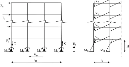
In a simplified form, the overturning moment at the building base can be determined by:
Figure 4-1. Schematic representation of the simplified design approach used for this study
∑
= FiHi
OTM (4.1)
Therefore assuming that for a regular frame structure (Figure 4-1 and Figure 4-2) significant variations in seismic axial load only occur in the outside columns, the following relation can be rearranged and used to find the seismic axial tension force T in the outer column.
B
B T L
M
OTM =
∑
+ ⋅ (4.2)Note that the proportion of overturning moment resisted by column base bending, ΣMB,
is an arbitrary design decision. Priestley and Kowalsky (2000) assume a point of MB, MB MB, MB,
C T
Fn
Fi
F1
Hi
H MB, MB
Vb
Vb
Vb
Vb
lB
VB
contraflexure in the bottom storey columns of 0.6H1 from the base. Therefore the
column base flexural contribution for k columns is:
(
1)
2
1 M ... M V 0.6H
M
MB = + + + k = B
∑
(4.3)As the outer column tension force is the sum of the seismic beam shears up the building ; it is possible to determine a distribution of beam shears, which under the assumption of seismically dominated beam flexural behaviour can be used to calculate the beam end moment demands. While the distribution of beam shears is also an arbitrary decision, and to some extent appears to have minimal influence, it is proposed that these forces be allocated in proportion to the column storey shear of the level below the beam level
∑
= bi
c V
T
i being considered, which can be represented as the following:
∑
=− −
= n
i i i C
i i C Bi
V V T V
1 1 , ,
1 ,
, with
∑
= − =
n j
j j i
i
C F
V
1 1 , ,
=
(4.4)
Here j denotes the storey below the beam level being considered and VC,i,i-1 is the storey
shear force below the particular beam level. With the seismic beam shears defined, the corresponding beam end moments at the column centreline are simply:
2 b bi bi
l V
M = (4.5)
These seismic beam moments are taken as the design moments for the members, with the assumption of moment-redistribution being used to account for gravity moment contribution. However in some cases this may not be appropriate, particularly when dealing with long-span beams that are dominated by gravity load demands.
To assign moment distributions to the columns, the proportion of base shear β resisted by each column must be decided. This is a design decision and will vary for different structures, however, for the case of the regular frames used in this study, proportions were set such that the moment distributions were close to those found using an elastic lateral force analysis. For the frames studied, where four columns were present (Figure 4-2), the proportions were kept at 0.17VB to each of the outside columns and 0.33VB to
each inside column.
To derive the distribution of moments above the column base, joint equilibrium was maintained using the cumulative storey shear found by Eq.(4.4). Thus having set the individual column base moment as:
(
1)
, V 0.6H
MBk =β⋅ B (4.6)
the bottom storey top moment Mi,top,kcan be found to satisfy the value of βVB and
therefore knowing the first floor beam moment, by equilibrium the value of the column design moment above the first floor joint can be calculated so that:
k top i bi k bottom
i M M
M +1, , = − , , (4.7)
In a similar fashion to the first storey column, the second storey top moment can be found from:
k bottom i i i C k top
i V h M
M +1, , =β , ⋅ +1− +1, , (4.8)
The process follows in the same manner to each successive storey above. It is possible that initial assumptions of base shear distribution between columns may produce unrealistic bending moment distributions in the upper levels of the frame, in which case the proportions can be adjusted to achieve values suitable for design.
Having determined the design moments and shears for the frame, it is then a matter to develop the reinforcement detailing suitable for the given demands, as follows using current methods of reinforced concrete Capacity Design.
4.2 DESIGN PROCEDURE AS APPLIED TO THIS STUDY
4.2.1 Frame Descriptions
The intent of this study was to assess the dynamic behaviour of moment resisting reinforced concrete perimeter frames, or ‘tube-frames’ that have become a common form of lateral force resistance. These frames are generally characterised by the use of short spans with deeper than usual beams, relative to the columns. Thus they are comparatively stiff, commonly with a low yield displacement. In comparison the internal frames for such systems are required only for gravity support, and are therefore more slender and flexible.
For this study the following frame properties (Table 4-1) and geometries (Table 4-4) were used, with values of concrete compressive strength f ’c and steel yield strength fy defined so
that material overstrength was already accounted for in the design and therefore could be ignored in looking at the results from the analyses. The Modulus of Elasticity for concrete was calculated using 4700 '
c
c f
Table 4-1. Basic material parameters assumed in frame design and modelling
Property fc’ Ec ρ ν fy εy
Value 35 MPa 27800 MPa 2.4 t/m3 0.3 450 MPa 0.00225
The definition of a tube-frame implies that under seismic attack, the exterior frames provide the dominant form of lateral resistance. Therefore, in this study the seismic weights are somewhat higher than are expected for normal flexible frames. Table 4-2 outlines how the seismic weight was assumed to be distributed up the height of the structure, to represent dead and live load contributions.
Table 4-2. Frame seismic weight parameters
Levels n Seismic Weight Gravity Weight
Roof: n 2500 kN 1250 kN
All levels: 1 to n-1 3000 kN 1500 kN
Thus the frames are modelled as lumped mass systems, with the mass at each level mass being distributed to the beam-column joints to represent the proportion carried laterally and vertically, based on tributary member lengths. To these weights the beam and column self weights are added at each joint in a similar fashion.
Figure 4-2 schematically presents the six frames investigated, ranging from two to twenty storeys in height, with a constant inter-storey height of 3.5 meters and beam span length of 5 meters for all beam bays. Table 4-4 defines the beam and column section sizes used at each level in each of the frames.
4.2.2 Displacement Design Spectrum
The design displacement spectrum was defined using the forthcoming version of EC8 (based on the May 2002 draft). Previous studies using direct displacement-based design have tended to use values of Peak Ground Acceleration around 0.4g, however for this study a somewhat higher value of 0.6g was used with the assumption of “moderately soft ground” which can be characterised by Soil Type B.
Therefore to generate the generic 5% damping, elastic response spectrum the following parameters apply:
Table 4-3. EC8 elastic response spectrum parameters for Soil Type B
PGA S γ η Tb Tc Td
0.6g 1.2 1 1 0.15 0.5 5
Note that the corner period of the displacement spectrum that can be derived from the acceleration spectrum was extended to 5 seconds, from the code specified maximum of 2 seconds. This is because for large magnitude earthquakes found in many regions of the world, the assumption of constant displacement demand for structural periods beyond 2 seconds, has been found inappropriate (Faccioli et al., 2004) and is summarised with respect to direct displacement-based design by Priestley et al. (2004). Also, the use of an effective period as defined in Section 3.1.1 can require the extension of the design displacement spectrum in order to accommodate differences in response due to the influence of ductility, as effective periods can be significantly longer than the corresponding elastic period (Priestley and Kowalsky, 2000).
Based on the following equations [ Eq.(4.9) ] defined in EC8, the design spectrum is presented in Figure 4-3.
0≤T≤T : B
( )
(
)
⎥⎦ ⎤ ⎢
⎣ ⎡
− ⋅ ⋅ + ⋅ ⋅ ⋅
= γ 1 η 2.5 1
B g
e
T T S
a T S
TB≤T≤T :C Se
( )
T =ag⋅S⋅γ⋅η⋅2.5TC≤T≤T :D
( )
⎥⎦ ⎤ ⎢ ⎣ ⎡ ⋅ ⋅ ⋅ ⋅ =
T T S
a T
Se g γ η 2.5 C
T≥TD:
( )
⎥⎦ ⎤ ⎢ ⎣ ⎡ ⋅ ⋅ ⋅ ⋅ =
2
5 . 2
T T T S
a T
Se g γ η C D
(4.9)
The design spectral accelerations can then be converted to the design displacement spectrum using the relation in Eq.(4.10).
( )
22 ⎟⎠
⎞ ⎜ ⎝ ⎛ ⋅ =
π T T S
Note:
Columns defined as i = 1, 2, 3, 4 from left to right on diagrams Columns are square sections Further dimension details given in Table 4-4 below
8 @ 3
.5 m
Figure 4-2. Building frame geometries
4 @ 3
.5 m
2 @ 3
.5 m
Frame C Frame B
Frame A
12 @ 3
.5 m
16 @ 3
.5 m
20 @ 3
.5 m
Frame E
Table 4-4. Frame member geometries n Fr am e A Fra m e B Frame C Frame D Fra m e E Frame F Co lu m ns (s qu are ) Bea m s Col um ns (s qu ar e) Bea m s Col um ns (s qu ar e) Be am s Co lu m ns (s qu ar e) Bea m s Col um ns (s qu ar e) Bea m s Col um ns (s quare ) Bea m s i 1& 2 3& 4 bw hb 1& 2 3& 4 bw hb 1& 2 3& 4 bw hb 1& 2 3& 4 bw hb 1& 2 3& 4 bw hb 1& 2 3& 4 bw hb 20 950 95 0 40 0 90 0 19 950 95 0 40 0 90 0 18 950 95 0 40 0 90 0 17 950 95 0 40 0 90 0 16 850 850 40 0 90 0 950 95 0 40 0 90 0 15 850 850 40 0 90 0 950 95 0 40 0 90 0 14 850 850 40 0 90 0 950 95 0 40 0 12 00 13 850 850 40 0 90 0 950 95 0 40 0 12 00 12 80 0 80 0 400 90 0 850 850 40 0 90 0 950 95 0 40 0 12 00 11 80 0 80 0 400 90 0 850 850 40 0 90 0 950 95 0 40 0 12 00 10 80 0 80 0 400 9 00 850 850 40 0 12 00 950 95 0 40 0 1 20 0 9 80 0 80 0 400 9 00 850 850 40 0 12 00 950 95 0 40 0 1 20 0 8 70 0 700 40 0 900 80 0 80 0 400 9 00 850 850 40 0 12 00 950 95 0 40 0 1 40 0 7 70 0 700 40 0 900 80 0 80 0 400 9 00 850 850 40 0 12 00 950 95 0 40 0 1 40 0 6 70 0 700 40 0 900 80 0 80 0 400 9 00 850 850 40 0 12 00 950 95 0 40 0 1 40 0 5 70 0 700 40 0 900 80 0 80 0 400 9 00 850 850 40 0 12 00 950 95 0 40 0 1 40 0 4 70 0 70 0 40 0 90 0 70 0 700 40 0 900 80 0 80 0 400 9 00 850 850 40 0 12 00 950 95 0 40 0 1 40 0 3 70 0 70 0 40 0 90 0 70 0 700 40 0 900 80 0 80 0 400 9 00 850 850 40 0 12 00 950 95 0 40 0 1 40 0 2 650 650 400 9 00 70 0 70 0 40 0 90 0 70 0 700 40 0 900 80 0 80 0 400 9 00 850 850 40 0 12 00 950 95 0 40 0 1 40 0 1 650 650 400 9 00 70 0 70 0 40 0 90 0 70 0 700 40 0 900 80 0 80 0 400 9 00 850 850 40 0 12 00 950 95 0 40 0 1 40 0 NB
: bw
is th e b ea m s hea r w id th
; h
b is th e tota l be am d epth
EC8 Design Spectra: Soil Type B PGA 0.6g
0.00 0.20 0.40 0.60 0.80 1.00 1.20 1.40 1.60 1.80 2.00 2.20
0.0 0.5 1.0 1.5 2.0 2.5 3.0 3.5 4.0 4.5 5.0 5.5 6.0
Period (sec)
SA
(
g
)
0 200 400 600 800 1000 1200 1400
SD
(m
m
)
5% EC8 Accn 5% EC8 Disp
Figure 4-3. EC8 5% Acceleration and Displacement Spectra for Soil Type B (modified for a Corner Period = 5.0 seconds) ; PGA = 0.6g
The parameters ∆C,5 and Tc used in Eq.(3.8) at the 5% damping level, are 1.118 meters
and 5 seconds respectively.
4.2.3 Direct Displacement-based Design Parameters
The key objective of this study is to develop a method of accounting for higher mode amplification in reinforced concrete frames that does not require the need for inelastic time-history analysis. Therefore a critical design inter-storey drift of θ = 2% was assigned, in accordance with the recommendations in NZS 4203. For a constant storey height of 3.5 meters, this corresponds to an inter-storey displacement of 0.07 meters at the critical storey level, assumed to be the lowest level.
The yield displacements, ductilities and equivalent viscous damping values were calculated at each level and combined using Eq.(3.15) to give the substitute structure effective damping level. Finally using Eqs.(3.8) to (11) the following direct displacement-based design parameters were found for each frame, as shown in Table 4-5.
Table 4-5. Direct displacement-based design parameters for initial study frames
Frame θd ∆d Me He ξeff Te Ke Vb
(m) (t) (m) (%) (sec) (kN/m) (kN)
A: n = 2 2 % 0.114 547 5.7 21.8 0.83 31191 3542
B: n = 4 2 % 0.205 1066 10.2 21.8 1.50 18701 3828
C: n = 8 2 % 0.317 2216 19.0 17.6 2.13 19276 6103
D: n = 12 2 % 0.465 3266 28.1 17.4 3.11 13338 6196
E: n = 16 2 % 0.613 4382 37.2 18.6 4.21 9761 5979
F: n = 20 2 % 0.721 5515 46.2 19.0 5.35 8710 6281
NB: Te for Frame F exceeds Tc therefore iteration was required for actual displacement and equivalent damping
The variation in equivalent viscous damping values is a reflection of the changes in design displacement profile, with the large difference between Frames B and C due to the introduction of the parabolic profile for n > 4. However the increase in the damping value for the 16 and 20 storey frames is due to an error in the calculation of the weighted average, later found in the design calculations and is explained further in Chapter 6.
With these parameters defined, the equivalent lateral force distributions and overturning moments were calculated. The method described in Section 4.1 is then used with values of base shear proportion β, to give sensible column bending moment distributions. The equivalent lateral forces, storey shears and overturning moment distributions are given in Table 4-6 and Table 4-7, resulting member design bending moments and shears in Table 4-8 and Table 4-9, and comparatively in Figure 4-4.
Table 4-6. DDBD equivalent lateral forces, storey shears, overturning moments and displacements; Frames A, B & C
Storey Fi Vicol O TM ∆i Fi Vicol O TM ∆i Fi Vicol O TM ∆i
(kN) (kN) (kNm) (m) (kN) (kN) (kNm) (m) (kN) (kN) (kNm) (m)
20 19 18 17 16 15 14 13 12 11 10 9
8 865 865 0 0.498
7 936 1800 3027 0.443
6 816 2616 9329 0.387
5 692 3308 18487 0.328
4 1357 1357 0 0.280 563 3871 30065 0.267
3 1236 2592 4748 0.210 429 4300 43613 0.203
2 2215 2215 0 0.140 824 3416 13820 0.140 291 4591 58663 0.138
1 1349 3564 7753 0.070 412 3828 25775 0.070 148 4738 74731 0.070
0 0 3564 20228 0.000 0 3828 39172 0.000 0 4738 91315 0.000
Frame A Frame B Frame C
Table 4-7. DDBD equivalent lateral forces, storey shears, overturning moments and displacements; Frames D, E & F
Store y Fi Vicol O TM ∆i Fi Vicol O TM ∆i Fi Vicol O TM ∆i
(kN) (kN) (kNm) (m) (kN) (kN) (kNm) (m) (kN) (kN) (kNm) (m)
20 707 707 0 0.718
19 826 1532 2474 0.716
18 819 2352 7838 0.711
17 809 3161 16069 0.702
16 693 693 0 0.717 795 3956 27133 0.689 15 825 1518 2424 0.697 776 4732 40977 0.673 14 798 2316 7737 0.674 763 5494 57538 0.653 13 767 3083 15844 0.648 735 6229 76767 0.630 12 732 732 0 0.643 732 3815 26635 0.618 704 6933 98569 0.603 11 842 1575 2562 0.606 693 4508 39989 0.585 668 7601 122836 0.573 10 787 2361 8073 0.566 658 5166 55768 0.549 628 8230 149441 0.538 9 727 3088 16337 0.523 610 5776 73849 0.509 584 8814 178246 0.501 8 662 3750 27144 0.477 559 6335 94066 0.466 541 9355 209096 0.459 7 594 4344 40270 0.427 503 6838 116239 0.419 488 9843 241838 0.415 6 522 4866 55474 0.375 443 7281 140171 0.370 431 10274 276289 0.366 5 445 5311 72505 0.320 379 7660 165654 0.316 370 10643 312247 0.314 4 364 5675 91093 0.262 312 7972 192465 0.260 304 10947 349498 0.258 3 279 5955 110956 0.201 240 8211 220366 0.200 234 11182 387814 0.199 2 190 6145 131798 0.137 164 8375 249106 0.137 161 11342 426951 0.136 1 97 6242 153306 0.070 84 8459 278419 0.070 82 11425 466649 0.070 0 0 6242 175154 0.000 0 8459 308026 0.000 0 11425 506635 0.000
Table 4-8. Beam design shear forces and bending moments
Store y Vbi Mbi Vbi Mbi Vbi Mbi Vbi Mbi Vbi Mbi Vbi Mbi
(kN) (kNm) (kN) (kNm) (kN) (kNm) (kN) (kNm) (kN) (kNm) (kN) (kNm)
20 157 393
19 341 852
18 523 1307
17 703 1757
16 152 381 879 2198
15 334 834 1052 2629
14 509 1273 1221 3053
13 678 1695 1385 3462
12 158 395 839 2097 1541 3853
11 340 850 991 2478 1690 4224
10 510 1274 1136 2840 1829 4573
9 667 1666 1270 3175 1959 4898
8 180 450 810 2024 1393 3482 2079 5199
7 374 936 938 2344 1503 3759 2188 5470
6 544 1360 1050 2626 1601 4002 2284 5709
5 688 1719 1146 2866 1684 4211 2366 5915
4 252 629 805 2012 1225 3063 1753 4382 2433 6084
3 481 1202 894 2235 1285 3214 1805 4514 2486 6214
2 326 814 633 1584 954 2386 1327 3316 1842 4604 2521 6303
1 524 1310 710 1775 985 2463 1348 3369 1860 4650 2540 6349
Co lumn Te ns io n
F o rc e 850 - 2076 - 5424 - 10803 - 19351 - 32176
-Frame C Frame D Frame E Frame F
Frame A Frame B
4.2.4 Section Analysis
For the inelastic time-history analyses, it was required to design the reinforcing details in both the columns and beams. This was accomplished using the GW-BASIC program, RECMAN2, that implements the concrete confinement and reinforcement stress-strain model presented by Mander et al. (1988). This program was used to calculate reinforcement requirements, and then to perform a moment-curvature analysis on the section with the designed reinforcement layout.
A bilinear approximation was made to the moment-curvature curve following the definitions of Paulay and Priestley (1992) for yield curvature, nominal moment capacity, ultimate curvature and ultimate capacity. For this process the limiting material strains suggested in Section 3.1.1 were applied and are summarised in Table 4-10. While RECMAN2 calculates the confinement effect of the steel design, according to the equation in Table 4-10, the ultimate concrete compression strain resulting from the assumed transverse reinforcement was manually checked for each frame.
Table 4-9. DDBD column moment distributions for Outer (1 & 4) and Inner (2 & 3) columns (kNm; positive values are anticlockwise moment)
Store y O ute r Inne r O ute r Inne r O ute r Inne r O ute r Inne r O ute r Inne r O ute r Inne r
20 2002 823
19 -1581 1640
19 2433 64
18 -1521 1706
18 2828 908
17 -1428 1809
17 3185 1704
16 -1304 1947
16 1348 206 3502 2450
15 -936 1006 -1149 2119
15 1771 663 3778 3140
14 -867 1090 -963 2325
14 2141 1456 4016 3781
13 -762 1219 -747 2565
13 2457 2170 4209 4359
12 -623 1391 -502 2836
12 449 736 2720 2804 4355 4870
11 -21 117 -450 1603 -230 3138
11 871 1582 2928 3353 4454 5310
10 49 253 -246 1854 69 3470
10 1225 2296 3085 3826 4505 5677
9 155 456 -12 2141 392 3828
9 1511 2877 3187 4209 4506 5968
8 294 722 250 2462 738 4212
8 1534 186 1730 3326 3232 4502 4460 6185
7 -990 1154 462 1045 537 2815 1106 4620
7 1925 717 1883 3644 3221 4703 4364 6319
6 -791 1299 656 1419 847 3195 1493 5049
6 2151 1421 1970 3832 3155 4810 4216 6369
5 -503 1510 875 1839 1177 3600 1896 5497
5 2222 1929 1992 3894 3034 4822 4018 6332
4 -138 1776 1113 2296 1524 4026 2315 5961
4 1667 220 2150 2248 1950 3829 2858 4738 3769 6206
3 -717 1204 289 2088 1367 2785 1885 4469 2745 6438
3 1919 1199 1946 2382 1847 3642 2629 4558 3469 5990
2 -104 1522 763 2434 1634 3298 2257 4926 3184 6925
2 1239 1203 1688 1645 1623 2339 1682 3335 2347 4282 3119 5681
1 312 1123 703 1942 1269 2803 1909 3828 2637 5392 3630 7419
1 998 1497 1072 1608 1194 2123 1459 2910 2013 3908 2719 5278
0 1497 2245 1608 2411 1791 3184 2189 4365 3020 5862 4079 7917
Frame A Frame B Frame C Frame D Frame E Frame F
For the purposes of consistency, the transverse steel detailing was assumed to remain constant throughout the structure, for each frame, however, it was set so that basic requirements specified in NZS 3101 were satisfied. Thus with the assumption that longitudinal reinforcing has a nominal diameter (db) of 28mm, the required maximum
spacing was the smaller of 6db or d/4; in all cases the former governed, and under
practical considerations the transverse reinforcement centre to centre spacing was set at 150mm.
Displacement Based Design Overturning Moment Profiles 0 7 14 21 28 35 42 49 56 63 70
0 200000 400000 600000
O ve rturning Mome nt (kNm)
He ig h t ( m ) Frame A Frame B Frame C Frame D Frame E Frame F
Displacement Based Design Distribution of Shear Forces 0 7 14 21 28 35 42 49 56 63 70
0 5000 10000 15000
She ar (kN)
He ig h t ( m ) Frame A Frame B Frame C Frame D Frame E Frame F
Displacement Based Design Displacement Profiles 0 7 14 21 28 35 42 49 56 63 70
0.000 0.200 0.400 0.600 0.800
Displ ace me nt (m)
He ig h t ( m ) Frame A Frame B Frame C Frame D Frame E Frame F
Displacement Based Design Distribution of Drifts (% )
0 7 14 21 28 35 42 49 56 63 70
0.0% 0.5% 1.0% 1.5% 2.0% 2.5%
Drift (%) He ig h t ( m ) Frame A Frame B Frame C Frame D Frame E Frame F
Table 4-10. Limiting material strain conditions to determine bilinear approximation to Moment-Curvature relations
Concrete: εc Steel: εs ‘First Yield’: M & y φy’ 0.002 fy/Es = 0.00225
‘Nominal Capacity’: MN 0.004 0.015
‘Yield’: φy Extrapolated from origin through ‘First Yield’ to MN ‘Ultimate Capacity’: MN
& φu
(
)
'
4 . 1 004 . 0
cc suh yh s cm
f
f ε
ρ
ε = + 0.6εsu = 0.06
Mander et al. (1988) proposed the following equation to calculate the confined concrete strength:
' '
' '
' ' 1.254 2.254 1 7.94 2
c c
l c
l
cc f
f f f
f f
⎟⎟ ⎟ ⎠ ⎞ ⎜⎜
⎜ ⎝ ⎛
− +
+ −
= (4.11)
where f ’l is applied using lx e x yh and ly e y yh to account for different
confinement levels in orthogonal directions. For this study the confinement in each direction was considered equal.
f K
f' = ρ f' =K ρ f
Preliminary trials of the frame designs suggested that the moment-curvature behaviour of the beams did not vary significantly, in particular the post yield stiffness of the section was found to be reasonably consistent. Therefore it was considered appropriate to set the ratio of the bilinear moment-curvature post-yield stiffness to initial stiffness, rφ, equal to 0.015 for the beams.
As described by Priestley (2003), the initial flexural stiffness can be determined using the bilinear approximation to the moment-curvature curve:
y c
N cr
E M I
φ
= (4.12)
Using the simplified equation for the yield curvature in T-section beams proposed by Priestley (1998):